13 Population-adjusted indirect comparisons
David M. Phillippo
University of Bristol, UK
Jeroen P. Jansen
University of California San Francisco, USA
Antonio Remiro-Azócar
Novo Nordisk, Spain
Howard Z. Thom
University of Bristol, UK
13.1 Introduction
Standard network meta-analysis (NMA) and indirect comparison methods, as discussed in Chapter 10, are widely used to estimate relative treatment effects between multiple treatments of interest from several randomised controlled trials. However, these methods assume that any effect-modifying variables—those that alter the effect of treatment relative to control—are balanced between the populations of the included trials and with the target population of interest. In this chapter, we explore a recent and increasingly popular class of methods for relaxing this assumption, that aim to account for effect modifiers in order to create population-adjusted estimates. These methods are primarily concerned with adjusting for participant characteristics that may be effect modifiers; differences in study-level effect modifiers related to the design or context of the trials such as treatment administration or co-treatments are also a concern for the validity of analyses, however these are typically perfectly confounded at the study level and may require alternative adjustment methods. Population adjustment approaches are also used to incorporate single-arm studies or connect disconnected networks, under much stronger assumptions. Population adjustment methods are seeing increasing use in HTA submissions (Phillippo et al., 2019; Remiro-Azócar et al., 2021a; Serret-Larmande et al., 2023), in no small part due to the proliferation of single-arm studies for licensing approval (Hatswell et al., 2016).
We begin by outlining the assumptions required by these methods. We then describe current methods depending on the level of individual participant data (IPD) available: i) full IPD; ii) IPD from some studies, and aggregate data (AgD) from others; and iii) no IPD, only AgD from all studies. We give most attention to the mixed IPD and AgD case, which is the most common in HTA. We primarily focus on scenarios with connected networks of randomised controlled trials, but highlight the additional assumptions and implications for scenarios involving single-arm studies or disconnected networks of trials. We refer interested readers to Technical Support Document 18, published by the NICE Decision Support Unit, for further details and recommendations on the use of population adjustment methods in HTA (Phillippo et al., 2018, 2016).
13.2 Assumptions and definitions
Effect modifiers are variables that alter the relative effect of treatment compared to control, as measured on a given scale (e.g. odds ratios, hazard ratios), so that treatment is more or less effective depending on the level of the effect modifier. Prognostic factors are variables that affect outcomes on all treatments equally. Covariates may be either prognostic or effect-modifying, or both, and their definition and interpretation is specific to the chosen effect measure scale. Network meta-analysis, along with pairwise meta-analysis and indirect comparison as special cases, relies on an assumption of exchangeability; that relative treatment effects are the same across all included studies, even if unobserved. In a population-adjustment context, we refer to this as constancy of relative effects: the relative effects are assumed constant across the included study populations (or drawn from the same distribution, in a random effects model). This assumption may be violated if there are effect modifiers present, leading to biased estimates from NMA. Moreover, even if effect modifiers are balanced between all study populations, if these do not represent the target population for a treatment decision then the NMA estimates may still be biased for that target population. For decision making, estimates must be produced that are relevant to the decision target population. The target population need not be represented by one of the studies in the network, indeed the target population may be best represented by a comprehensive registry or cohort study in the population (Phillippo et al., 2016).
With population adjustment methods, we aim to estimate relative treatment effects for a target population of interest. In the case of a connected network, population adjustment methods aim to account for effect-modifying variables, for example by outcome regression or reweighting, thereby relaxing the constancy assumption to conditional constancy of relative effects (Phillippo et al., 2016). In other words, we assume that relative treatment effects can be predicted across populations based on the included effect modifiers. This requires that all effect modifiers have been included and correctly specified in the analysis, and may be violated if there are unobserved effect modifiers that are unbalanced between populations. This assumption may also be violated if effect modifying terms in the model are misspecified; for example if the true outcome model involves a non-linear treatment-covariate interaction, and a linear interaction term is included in an outcome regression approach or only means are matched in a reweighting approach. This assumption can also be violated when using a non-collapsible effect measure (such as an odds ratio or hazard ratio) if baseline risk differs between populations, in which case prognostic variables may also need to be adjusted for. The concept of a target population becomes especially important when population adjustment is considered. If effect modification is present, then treatment effects can vary between populations, and therefore treatment decisions may also vary between populations. Thus any suitable population adjustment method must be able to produce estimates that are relevant for the target population of interest.
Population adjustment methods may also be used to incorporate single-arm studies or disconnected evidence networks, under a much stronger assumption of conditional constancy of absolute effects (Phillippo et al., 2016). We refer to such analyses as unanchored, since there is no common comparator arm with which to anchor the analyses, unlike population adjustment in connected networks which are anchored by common comparators. This assumption requires that absolute outcomes can be predicted across populations, by correctly accounting for all prognostic and effect-modifying covariates. This is widely considered to be very hard to achieve; if this were straightforward, then there would be no need for randomised controlled trials. Decision-makers have justifiably treated unanchored analyses with strong caution, often seeking greater cost-effectiveness to offset the increased decision risk (Phillippo et al., 2019). Again, even if absolute outcomes can be adequately predicted and conditional constancy of absolute effects is satisfied, estimates must be produced for the target population of interest in order to be relevant for decision-making.
13.3 Methods with full IPD
In an ideal scenario, IPD are available from every study. In this case, in anchored scenarios with a connected network of randomised controlled trials, the “gold standard” approach is IPD network meta-regression adjusting for effect modifiers (Berlin et al., 2002; Lambert et al., 2002; Riley et al., 2023, 2010). Such analyses can be performed in various software packages, including the multinma R package (Phillippo, 2024). The multinma code to perform an IPD NMA looks very similar to that for mixed IPD and AgD which we will demonstrate in the next section (the main difference is that no AgD are present, so there is no need for set_agd_arm() or add_integration()). For unanchored scenarios involving single-arm studies or observational data, a range of methods drawn from the causal inference literature may be used; a detailed overview is given in NICE Decision Support Unit Technical Support Document 17, along with recommendations for use in HTA (Faria et al., 2015). Having IPD available from every study is very rare in HTA, so we refer interested readers to the above references for further information.
13.4 Methods with mixtures of IPD and AgD
In the context of HTA, IPD are (at best) available for a subset of studies relevant to the analysis, whilst only AgD are available for the remaining studies. For example, a manufacturer making a submission to a regulatory body is likely to have IPD on their own studies, but only published AgD from studies by their competitors. Several population adjustment methods have been proposed in this mixed data setting, which can largely be categorised as either reweighting-based or regression-based approaches.
13.4.1 Matching-Adjusted Indirect Comparison
Matching-Adjusted Indirect Comparison (MAIC) is a reweighting approach, where weights are derived for individuals in an IPD study to match the summary statistics of covariates in an AgD study (Ishak et al., 2015; Signorovitch et al., 2012, 2010). MAIC is designed for a two-study scenario, where in an anchored setting there is a single IPD study comparing treatment \(B\) with \(A\), and a single AgD study comparing treatment \(C\) with \(A\). The aim is to obtain a comparison of treatment \(C\) with \(B\) in the \(AC\) population.
The IPD study reports outcomes \(y_{ik(AB)}\) and covariates \(\boldsymbol{x}_{ik(AB)}\) for each individual \(i\) receiving treatment \(k\), where the subscript in brackets indicates the study population. The AgD study reports an estimated relative treatment effect \(\hat{\Delta}_{AC(AC)} = g(\bar{y}_{C(AC)}) - g(\bar{y}_{A(AC)})\) with standard error \(s_{AC(AC)}\), and summary covariate statistics \(\bar{\boldsymbol{x}}_{(AC)}\). The relative treatment effect is taken on a suitable transformed scale given by the link function \(g(\cdot)\), for example the logit link function for binary outcomes, which transforms the observed mean outcomes \(\bar{y}_{A(AC)}\), \(\bar{y}_{C(AC)}\) onto the comparison scale.
MAIC estimates the expected outcomes \(\hat{y}_{k(AC)}\) on treatments \(k=A,B\) in the \(AC\) population as a weighted average of the individual outcomes in the \(AB\) population: \[ \hat{y}_{k(AC)} = \frac{ \sum_{i} y_{ik(AB)} w_{ik} }{ \sum_{i} w_{ik} } \tag{13.1}\] The participant weights \(w_{ik}\) are typically derived using the method of moments (Signorovitch et al., 2010). This is equivalent to a minimisation problem, where we seek to minimise the overall difference between the reweighted covariate distribution and the AC summary statistics. Signorovitch et al. (2010) show that, after centering the covariates so that \(\bar{\boldsymbol{x}}_{(AC)} = \boldsymbol{0}\), this minimisation problem can be written as \[ \hat{\boldsymbol{\alpha}} = \operatorname*{argmin}_{\boldsymbol{\alpha}} \sum_{k=A,B} \sum_{i} \exp( \boldsymbol{x}\tr_{ik} \boldsymbol{\alpha} ) \tag{13.2}\] The weights are then equal to \(\boldsymbol{w}_{ik} = \exp( \boldsymbol{x}\tr_{ik(AB)} \hat{\boldsymbol{\alpha}} )\). This method of moments approach has been shown to be equivalent to entropy balancing (Phillippo et al., 2020b), and other alternative weighting schemes have also been proposed (Jackson et al., 2020).
Using these reweighted estimates, MAIC then estimates the population-average marginal relative effect \(\Delta_{BC(AC)}\) of \(C\) vs. \(B\) in the \(AC\) population in an anchored population-adjusted indirect comparison as \[ \hat{\Delta}_{BC(AC)} = \hat{\Delta}_{AC(AC)} - \hat{\Delta}_{AB(AC)} \tag{13.3}\] where \(\hat{\Delta}_{AB(AC)} = g(\hat{y}_{B(AC)}) - g(\hat{y}_{A(AC)})\). In practice, instead of using equation Equation 13.1 directly, the estimated relative treatment effect \(\hat{\Delta}_{AB(AC)}\) of \(B\) vs. \(A\) in the \(AC\) population may be obtained using a weighted regression of outcomes on treatment fitted to the IPD in the \(AB\) study; this approach extends readily to other outcomes such as survival.
In an unanchored setting there is no common \(A\) arm, and the above process proceeds to derive the reweighted estimate \(\hat{y}_{B(C)}\), before forming the unanchored population-adjusted indirect comparison with the estimated absolute outcomes on treatment \(C\) in the \(C\) population, \[ \hat{\Delta}_{BC(C)} = g(\hat{y}_{C(C)}) - g(\hat{y}_{B(C)}) \tag{13.4}\] Adequate prediction of absolute outcomes \(\hat{y}_{B(C)}\) on treatment \(B\) in the \(C\) population not only requires accounting for differences in effect modifiers between populations, but also prognostic factors that affect outcomes. Variance estimation for MAIC is usually achieved through either bootstrapping or robust sandwich estimators (Efron and Tibshirani, 1993; Phillippo et al., 2016; Sikirica et al., 2013).
As a weighting approach, MAIC cannot extrapolate and thus the AgD \(AC\) population must have sufficient overlap with the IPD \(AB\) population. The approximate effective sample size \(\mathrm{ESS} = \frac{\left(\sum_{k=A,B} \sum_{i} w_{ik}\right)^2}{\sum_{k=A,B} \sum_{i} w_{ik}^2}\) and visual inspection of the weight distribution in a histogram are useful diagnostics, with any extreme weights or large reductions in ESS indicating poor overlap (Phillippo et al., 2016; Signorovitch et al., 2010). MAIC is designed with a two-study indirect comparison in mind, and does not readily generalise to larger networks of studies and treatments (Phillippo et al., 2016). Crucially for decision making, MAIC can only produce estimates for the AgD \(AC\) population without further assumptions (Phillippo et al., 2016), which may not reflect the decision target population. In HTA settings, this typically means that a manufacturer can only produce estimates in the population of their competitor’s trial.
13.4.2 Simulated Treatment Comparison
Simulated Treatment Comparison (STC) is an outcome regression approach, where a regression model fitted in the IPD study is used to produce predictions in the AgD study population (Caro and Ishak, 2010; Ishak et al., 2015). In an anchored STC, the predicted relative treatment effect of \(B\) vs. \(A\) in the \(AC\) population is used to form an anchored population-adjusted indirect comparison following Equation 13.3. In an unanchored STC, the predicted average absolute outcome on treatment \(B\) in the \(C\) population is used to form an unanchored indirect comparison following Equation 13.4.
Like MAIC, STC does not readily generalise to larger networks of studies or treatments, and can only produce estimates relevant to the AgD study population which may not be representative of the decision target population.
The most common form of anchored STC “plugs in” mean covariate values from the \(AC\) population to obtain predicted outcomes on treatment \(A\) and \(B\) (Phillippo et al., 2016). However, when the model is non-linear in the covariates this results in aggregation bias. Moreover, when the outcome measure is non-collapsible, such as log odds ratios or log hazard ratios, this results in a biased indirect comparison because the resulting conditional effect is not compatible with the marginal effect from the AC study (Remiro-Azócar et al., 2021a). The original simulation-based STC approach avoids these biases by simulating individuals from the \(AC\) study covariate distribution to calculate a marginal relative effect \(\Delta_{AB(AC)}\) (Caro and Ishak, 2010). However, the authors proposed keeping the simulated sample size the same as the original sample size of the \(AC\) study, which introduces additional simulation uncertainty. Remiro-Azócar et al. (2022) propose a more sophisticated simulation-based STC approach formalised in a G-computation framework that properly targets marginal treatment effects and appropriately captures uncertainty, with R code provided in the supplementary materials.
Instead of simulation, numerical integration may also be used to avoid aggregation and non-collapsibility biases by integrating predictions over the \(AC\) covariate distribution. This is the approach taken by multilevel network meta-regression, which we now turn to.
13.4.3 Multilevel Network Meta-Regression
Multilevel network meta-regression (ML-NMR) is a population adjustment method that generalises the “gold standard” IPD network meta-regression to scenarios where some studies only provide aggregate data (Phillippo et al., 2020a). ML-NMR is based on methods proposed in the ecological inference literature (Jackson et al., 2008, 2006), which were first adapted to special cases of NMA with binary covariates (Jansen, 2012) and then generalised (Phillippo et al., 2024, 2020a; Phillippo, 2019). An individual-level regression model is defined, exactly as in an IPD network meta-regression, which models outcomes for individuals \(i\) in study \(j\) receiving treatment \(k\): \[ \begin{aligned} y_{ijk} &\sim \pi_\mathrm{Ind}(\theta_{ijk}) \\ g(\theta_{ijk}) &= \eta_{jk}(\boldsymbol{x}_{ijk}) = \mu_j + \boldsymbol{x}\tr_{ijk} (\boldsymbol{\beta}_1 + \boldsymbol{\beta}_{2,k}) + \gamma_k \end{aligned} \tag{13.5}\] The individual outcomes are given a suitable sampling distribution \(\pi_\mathrm{Ind}(\cdot)\), with parameter \(\theta_{ijk}\) modelled on a transformed linear predictor scale via the link function \(g(\cdot)\). The linear predictor \(\eta_{jk}(\boldsymbol{x})\) has stratified study-specific intercepts \(\mu_j\) in order to preserve randomisation, prognostic covariate effects \(\boldsymbol{\beta}_1\), effect modifying treatment-covariate interactions \(\boldsymbol{\beta}_{2,k}\), and individual-level treatment effects \(\gamma_k\). We set \(\boldsymbol{\beta}_{2,A} = \boldsymbol{0}\) and \(\gamma_A = 0\).
To incorporate AgD evidence, this individual-level model is then integrated (i.e. averaged) over the summary covariate distributions in each AgD study to form the aggregate-level model: \[ \begin{aligned} y_{\bullet jk} &\sim \pi_\mathrm{Agg}(\theta_{\bullet jk}) \\ \theta_{\bullet jk} &= \int_\mathfrak{X} g^{-1}( \eta_{jk}(\boldsymbol{x}) ) f_{jk}(\boldsymbol{x}) d\boldsymbol{x} \end{aligned} \tag{13.6}\] We use the subscript \(\bullet\) to indicate aggregate-level quantities, distinguishing from their individual-level counterparts. Aggregate outcomes \(y_{\bullet jk}\) are given a suitable distribution \(\pi_\mathrm{Agg}(\cdot)\) with parameter \(\theta_{\bullet jk}\). The parameter \(\theta_{\bullet jk}\) is modelled via the marginalisation integral, which averages the individual-level model for outcomes on treatment \(k\) in study \(j\) over the joint covariate distribution \(f_{jk}(\boldsymbol{x})\). Correctly relating the individual and aggregate levels of the model together in this manner via the marginalisation integral avoids aggregation bias and non-collapsibility bias, which are incurred by other approaches that simply “plug in” mean covariate values, including some forms of STC (Phillippo et al., 2016) and previous approaches to combining IPD and AgD in a meta-regression setting (Donegan et al., 2013; Saramago et al., 2012; Sutton et al., 2008).
The marginalisation integral (Equation 13.6) can be evaluated by hand in some special cases (see the appendix of Phillippo et al., 2020a), however a general and practical solution is to use a numerical method such as Quasi-Monte Carlo integration (Phillippo et al., 2020a). Writing down the aggregate-level model in this manner assumes that the aggregate-level distribution has a known form, which is the case for many models (e.g. Normal, Bernoulli/Binomial, Poisson, Multinomial) but not all; one particularly important exception is models for survival analysis. However, ML-NMR can also be formulated in a fully general manner by directly considering the likelihood contributions from each level of the model, bypassing the need for the aggregate-level distribution to be known, allowing very general application of the ML-NMR framework—including for survival analysis (Phillippo et al., 2024; Phillippo, 2019).
Fitting the ML-NMR model does require the joint covariate distribution \(f_{jk}(\boldsymbol{x})\) to be known in each AgD study, but in practice this is unlikely to be available. Instead, marginal covariate summaries such as means and standard deviations or categorical proportions are typically published. The joint covariate distribution may be reconstructed from such marginal summaries, together with assumed forms for the marginal distributions and a correlation matrix, using copulae (Phillippo et al., 2020a). Typically, the covariate correlations and forms of the marginal distributions are taken from the IPD studies. Simulation studies have shown that the ML-NMR results are typically not sensitive to misspecification of these additional assumptions for reconstructing the joint covariate distribution (Phillippo et al., 2020c); however, a highly non-linear model or targeting marginal instead of conditional treatment effects may increase sensitivity to these assumptions.
Crucially for decision making, ML-NMR can produce population-adjusted estimates in any target population of interest (or subgroup thereof). For a target population \(P\) with joint covariate distribution \(f_{(P)}(\boldsymbol{x})\), population-average conditional treatment effects between any pair of treatments \(a\) and \(b\) are found by integrating contrasts of the linear predictor on each treatment over the joint covariate distribution: \[ \begin{aligned} d_{ab(P)} &= \int_\mathfrak{X} ( \eta_{b(P)}(\boldsymbol{x}) - \eta_{a(P)}(\boldsymbol{x}) ) f_{(P)}(\boldsymbol{x}) d\boldsymbol{x} \\ &= \bar{\boldsymbol{x}}_{(P)}\tr (\boldsymbol{\beta}_{2,b} - \boldsymbol{\beta}_{2,a}) + \gamma_b - \gamma_a \end{aligned} \tag{13.7}\] which collapses to an expression in terms of the mean covariate values \(\bar{\boldsymbol{x}}_{(P)}\) in population \(P\) due to linearity. This population-average conditional treatment effect can be interpreted as the average of the individual-level treatment effects in population \(P\), when moving the population from treatment \(a\) to \(b\). Calculation of \(d_{ab(P)}\) requires information only on effect-modifying covariates in the target population, and not on the distribution of prognostic factors or baseline risk.
Estimates of absolute outcomes are often of interest to decision makers, and are typically the necessary inputs to an economic model. For example, with a binary outcome these are average event probabilities \(\bar{p}_{k(P)}\) on each treatment \(k\) in the population \(P\). Using ML-NMR, these are obtained via the marginalisation integral as \[ \bar{p}_{k(P)} = \int_\mathfrak{X} g^{-1}( \eta_{k(P)}(\boldsymbol{x}) ) f_{(P)}(\boldsymbol{x}) d\boldsymbol{x} \tag{13.8}\] The full joint covariate distribution \(f_{(P)}(\boldsymbol{x})\) is required, and may in practice be reconstructed from reported marginal summaries as described above (Phillippo et al., 2020a). Calculation of average absolute outcomes requires information on the distribution of both effect modifying and prognostic covariates in the target population, as well as the distribution of individual-level baseline risk \(\mu_{(P)}\). Information on the individual-level baseline risk \(\mu_{(P)}\) is unlikely to be available in the target population \(P\), however a distribution on \(\mu_{(P)}\) can be obtained from a distribution on the average event probabilities on any given reference treatment \(\bar{p}_{A(P)}\) by inverting Equation 13.8.
Population-average marginal treatment effects can then be obtained from the average absolute predictions. For example, a population-average marginal log odds ratio between treatments \(b\) and \(a\) is given by \[ \Delta_{ab(P)} = \logit(\bar{p}_{b(P)}) - \logit(\bar{p}_{a(P)}) \tag{13.9}\] Marginal probit differences, risk differences or risk ratios can be obtained in a similar fashion. Population-average marginal treatment effects can be interpreted as the effect on the expected overall number of events in population \(P\) when moving the population from treatment \(a\) to \(b\). Like the average absolute outcomes on which they are based, calculation of population-average marginal effects requires information on the distribution of both effect modifying and prognostic covariates in the target population, as well as the distribution of baseline risk.
Unlike MAIC and STC, ML-NMR can synthesise networks of any size and with any number of IPD or AgD studies. ML-NMR extends the standard NMA framework, reducing to IPD network meta-regression when IPD are available from all studies, and to standard AgD NMA when no covariates are included in the model. When there are only a small number of AgD studies for a treatment, ML-NMR may require an additional identifying assumption to estimate the corresponding treatment-covariate interactions for this treatment. Interaction terms may be assumed common for a set of treatments, \(\boldsymbol{\beta}_{2,k} = \boldsymbol{\beta}_{2,\mathcal{T}}\) for all treatments \(k\) in the set \(\mathcal{T}\), which for example allows estimation of interactions to be shared with another treatment for which IPD are available or shared between several AgD treatments (Phillippo et al., 2020a). This shared effect modifier assumption may be reasonable if treatments are in the same class and share a mode of action, but otherwise is unlikely to hold. When this assumption cannot be made, in a two-study indirect comparison ML-NMR is limited like MAIC and STC to producing estimates for the AgD study population. However, in even moderately-sized networks this assumption may be assessed, for example by relaxing one covariate at a time (Phillippo et al., 2023), or removed entirely given sufficient data. Moreover, the key population adjustment assumption—conditional constancy of relative effects—may then be assessed using standard NMA techniques for detecting residual heterogeneity and inconsistency (as described in Chapter 10) within the ML-NMR framework (Phillippo et al., 2023).
The multinma R package (Phillippo, 2024) provides a suite of functionality for performing ML-NMR analyses, for a range of outcome types, as well as IPD meta-regression and AgD NMA as special cases.
13.4.4 Example: Plaque psoriasis
As an illustrative example, we will consider a network of treatments for moderate-to-severe plaque psoriasis. This example has been described in detail previously, initially analysed using MAIC (Strober et al., 2016; Warren et al., 2018) and then with ML-NMR (Phillippo et al., 2023, 2020a).
Evidence base
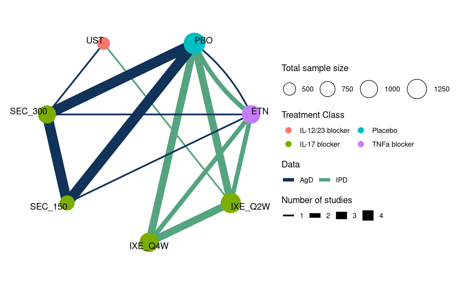
Nine studies compared ixekizumab (IXE) every two weeks (Q2W) or four weeks (Q4W), secukinumab (SEC) at 150 mg dose or 300 mg dose, ustekinumab (UST) at a weight-based dose, and etanercept (ETN), along with placebo (PBO) (Warren et al., 2018). These form the network shown in Figure 13.1. IPD were available from four studies (UNCOVER-1, -2, and -3, and IXORA-S), and published AgD were available from the remaining five studies (CLEAR, ERASURE, FEATURE, FIXTURE, JUNCTURE). Outcomes of interest included success/failure to achieve 75%, 95%, and 100% response on the psoriasis area and severity index (PASI) scale after 12 weeks; here we consider only the PASI 75 outcome, however Phillippo et al. (2023) demonstrate a joint analysis of all three outcomes in an ML-NMR model with ordered categorical distribution. Expert clinical opinion identified duration of psoriasis, previous systemic treatment, body surface area covered, weight, and psoriatic arthritis to be potential effect modifiers (Phillippo et al., 2020a; Strober et al., 2016); baseline summary statistics in each of the study populations are described in Tables 13.1 and 13.2.
The data are available in the multinma package (Phillippo, 2024): the dataset plaque_psoriasis_ipd provides IPD outcomes and covariates, and plaque_psoriasis_agd provides summary AgD outcomes and covariates.
# Load the multinma package to access the data
library(multinma)

# Inspect the datasets
head(plaque_psoriasis_ipd)
studyc trtc_long trtc trtn pasi75 pasi90 pasi100 age bmi pasi_w0 male bsa
1 IXORA-S Ixekizumab Q2W IXE_Q2W 2 1 1 1 62 38.6 15.8 FALSE 13
2 IXORA-S Ixekizumab Q2W IXE_Q2W 2 1 1 0 38 23.2 28.2 FALSE 37
3 IXORA-S Ixekizumab Q2W IXE_Q2W 2 1 1 0 54 27.5 13.2 TRUE 13
4 IXORA-S Ixekizumab Q2W IXE_Q2W 2 1 1 1 44 24.6 41.0 FALSE 67
5 IXORA-S Ixekizumab Q2W IXE_Q2W 2 1 1 0 44 28.3 15.2 FALSE 10
6 IXORA-S Ixekizumab Q2W IXE_Q2W 2 1 1 1 57 23.6 30.4 FALSE 75
weight durnpso prevsys psa
1 111.2 8 TRUE TRUE
2 62.0 1 TRUE FALSE
3 83.5 38 TRUE FALSE
4 66.0 1 TRUE FALSE
5 92.7 23 TRUE FALSE
6 73.5 21 TRUE FALSEhead(plaque_psoriasis_agd) studyc trtc_long trtc trtn pasi75_r pasi75_n pasi90_r pasi90_n
1 CLEAR Secukinumab 300 mg SEC_300 6 304 334 243 334
2 CLEAR Ustekinumab UST 7 265 335 179 335
3 ERASURE Placebo PBO 1 11 246 3 246
4 ERASURE Secukinumab 150 mg SEC_150 5 174 243 95 243
5 ERASURE Secukinumab 300 mg SEC_300 6 200 245 145 245
6 FEATURE Placebo PBO 1 0 59 0 59
pasi100_r pasi100_n sample_size_w0 age_mean age_sd bmi_mean bmi_sd pasi_w0_mean
1 130 334 337 45.2 13.96 29.1 5.87 21.7
2 86 335 339 44.6 13.67 29.0 6.69 21.5
3 2 246 248 45.4 12.60 30.3 7.80 21.4
4 31 243 245 44.9 13.30 29.8 6.80 22.3
5 70 245 245 44.9 13.50 30.3 7.20 22.5
6 0 59 59 46.5 14.14 NA NA 21.1
pasi_w0_sd male bsa_mean bsa_sd weight_mean weight_sd durnpso_mean durnpso_sd
1 8.50 68.0 32.6 17.78 87.4 19.95 19.6 12.90
2 8.07 74.3 32.0 16.80 87.2 22.11 16.1 11.24
3 9.10 69.4 29.7 15.90 89.7 25.00 17.3 12.40
4 9.80 68.6 33.3 19.20 87.1 22.30 17.5 12.00
5 9.20 69.0 32.8 19.30 88.8 24.00 17.4 11.10
6 8.49 66.1 32.2 17.39 88.4 21.55 20.2 14.22
prevsys psa
1 66.8 20.5
2 68.1 15.9
3 58.9 27.4
4 63.7 18.8
5 66.5 23.3
6 66.1 15.3We will demonstrate MAIC and ML-NMR analyses with this network. For illustrative purposes, we will consider the target population to be represented by the PROSPECT cohort study conducted in 335 sites across Germany (Thaçi et al., 2019), with covariate summary statistics given in Tables 13.1 and 13.2.
| CLEAR (AgD N = 676) |
ERASURE (AgD N = 738) |
FEATURE (AgD N = 177) |
FIXTURE (AgD N = 1306) |
IXORA-S (IPD N = 260) |
|
|---|---|---|---|---|---|
| Treatment arms | Secukinumab 300 mg Ustekinumab |
Placebo Secukinumab 150 mg Secukinumab 300 mg |
Placebo Secukinumab 150 mg Secukinumab 300 mg |
Placebo Etanercept Secukinumab 150 mg Secukinumab 300 mg |
Ixekizumab Q2W Ustekinumab |
| Age, years | 44.9 (13.8) | 45.1 (13.1) | 45.9 (14.0) | 44.5 (12.9) | 43.9 (12.5) |
| Body surface area, per cent | 32.3 (17.3) | 31.9 (18.3) | 32.0 (17.4) | 34.4 (18.9) | 32.0 (19.0) |
| Duration of psoriasis, years | 17.8 (12.2) | 17.4 (11.8) | 19.5 (13.1) | 16.5 (12.0) | 16.7 (11.7) |
| Male (%) | 71.2 | 69.0 | 66.1 | 71.1 | 64.6 |
| Baseline PASI score | 21.6 (8.3) | 22.1 (9.4) | 20.8 (8.3) | 23.7 (10.2) | 22.4 (9.5) |
| Previous systemic treatment (%) | 67.5 | 63.0 | 67.2 | 64.0 | 91.5 |
| Psoriatic arthritis (%) | 18.2 | 23.2 | 16.4 | 14.7 | 13.5 |
| Weight, kg | 87.3 (21.1) | 88.5 (23.8) | 91.6 (24.6) | 83.3 (20.9) | 87.8 (22.9) |
| JUNCTURE (AgD N = 182) |
UNCOVER-1 (IPD N = 1296) |
UNCOVER-2 (IPD N = 1219) |
UNCOVER-3 (IPD N = 1339) |
PROSPECT (AgD N = 1509) |
|
|---|---|---|---|---|---|
| Treatment arms | Placebo Secukinumab 150 mg Secukinumab 300 mg |
Placebo Ixekizumab Q2W Ixekizumab Q4W |
Placebo Etanercept Ixekizumab Q2W Ixekizumab Q4W |
Placebo Etanercept Ixekizumab Q2W Ixekizumab Q4W |
Secukinumab 300 mg |
| Age, years | 44.7 (13.9) | 46.3 (13.0) | 46.1 (12.8) | 45.6 (12.8) | 48.1 (13.7) |
| Body surface area, per cent | 27.4 (14.9) | 27.6 (17.5) | 26.5 (16.8) | 28.0 (16.4) | 18.7 (18.4) |
| Duration of psoriasis, years | 20.5 (13.5) | 20.0 (12.1) | 18.7 (12.1) | 17.8 (11.8) | 19.6 (13.5) |
| Male (%) | 68.7 | 67.5 | 67.7 | 68.3 | 62.4 |
| Baseline PASI score | 20.1 (7.5) | 20.3 (8.0) | 19.6 (7.1) | 20.9 (8.2) | 17.7 (12.5) |
| Previous systemic treatment (%) | 55.5 | 73.1 | 64.2 | 58.8 | 91.0 |
| Psoriatic arthritis (%) | 23.1 | 28.2 | 23.6 | 20.2 | 20.2 |
| Weight, kg | 91.6 (25.8) | 92.4 (24.8) | 91.7 (21.6) | 90.1 (22.6) | 87.5 (20.3) |
Anchored MAIC analysis
We recreate here a MAIC analysis previously performed in this network (Strober et al., 2016), comparing secukinumab 300 mg vs. ixekizumab Q2W via etanercept as a common comparator. Two IPD studies (UNCOVER-2 and -3) compare ixekizumab to etanercept, and one AgD study (FIXTURE) compares secukinumab to etanercept. We will derive weights for each of the UNCOVER studies to match their covariate distributions with the FIXTURE population. We implement the MAIC process described in Section 13.4.1. The code is adapted from NICE Decision Support Unit Technical Support Document 18 (Phillippo et al., 2016); interested readers may also investigate several R packages which largely build on this code (Gregory et al., 2023; hta-pharma, 2024; Lillian Yau, 2022; Young, 2022). We will perform the indirect comparison on the probit scale.
First, we prepare the data. We select the relevant rows from the IPD and AgD data sets, and check that there are no missing data.
# Select relevant rows
fixture_agd <- subset(
  plaque_psoriasis_agd,studyc == "FIXTURE" & trtc %in% c("ETN", "SEC_300")
)

uncover_ipd <- subset(
  plaque_psoriasis_ipd,
  studyc %in% c("UNCOVER-2", "UNCOVER-3") & trtc %in% c("ETN", "IXE_Q2W")
)

# Check for missing data in IPD
all(complete.cases(
  uncover_ipd[, c("pasi75", "durnpso", "prevsys", "bsa", "weight", "psa")])
)
[1] TRUEAs in Section Section 13.4.1, we first centre the covariates around the values in the AgD FIXTURE study. For continuous covariates, we will match on the first and second moments (i.e. mean and variance).
# FIXTURE AgD covariate summaries (first and second moments)
X_agd <- with(fixture_agd,
              cbind(durnpso_mean, durnpso_mean^2 + durnpso_sd^2,
                    prevsys / 100,
                    bsa_mean, bsa_mean^2 + bsa_sd^2,
                    weight_mean, weight_mean^2 + weight_sd^2,
                    psa / 100))

# We were given summaries by arm, so convert these to overall summaries
X_agd <- apply(
  X_agd, MARGIN = 2, FUN = weighted.mean, w = fixture_agd$sample_size_w0
)

# Create matrix of centred UNCOVER IPD covariates
X_ipd <- sweep(with(uncover_ipd,
                    cbind(durnpso, durnpso^2,
                          prevsys,
                          bsa, bsa^2,
                          weight, weight^2,
                          psa)),
               MARGIN = 2, STATS = X_agd, FUN = '-')
We then define the objective and gradient functions for optimisation to estimate the participant weights, as described in Equation 13.2:
# Objective function
objfn <- function(a1, X){
  sum(exp(X %*% a1))
}

# Gradient function
gradfn <- function(a1, X){
  colSums(sweep(X, 1, exp(X %*% a1), "*"))
}
We use optimisation to obtain weights for the UNCOVER studies. We do this separately for each study, to ensure that each is matched to the FIXTURE population.
study_ipd <- uncover_ipd$studyc

# Estimate weights for UNCOVER-2
opt_uncover2 <- optim(par = rep(0, ncol(X_ipd)),
                      fn = objfn, gr = gradfn,
                      X = X_ipd[study_ipd == "UNCOVER-2", ],
                      method = "BFGS")

a1_uncover2 <- opt_uncover2$par
wt_uncover2 <- exp(X_ipd[study_ipd == "UNCOVER-2", ] %*% a1_uncover2)

# Normalise to sum to ESS for interpretation
wt_uncover2 <- wt_uncover2 * sum(wt_uncover2) / sum(wt_uncover2^2)

# Estimate weights for UNCOVER-3
opt_uncover3 <- optim(par = rep(0, ncol(X_ipd)),
                      fn = objfn, gr = gradfn,
                      X = X_ipd[study_ipd == "UNCOVER-3", ],
                      method = "BFGS")

a1_uncover3 <- opt_uncover3$par
wt_uncover3 <- exp(X_ipd[study_ipd == "UNCOVER-3", ] %*% a1_uncover3)

# Normalise to sum to ESS for interpretation
wt_uncover3 <- wt_uncover3 * sum(wt_uncover3) / sum(wt_uncover3^2)
We can examine the histograms of the weights, and calculate the effective sample size.
hist(wt_uncover2, freq = FALSE, breaks = 50, main = NULL, xlab = "Weight")
hist(wt_uncover3, freq = FALSE, breaks = 50, main = NULL, xlab = "Weight")

# Effective sample sizes
sum(wt_uncover2)^2 / sum(wt_uncover2^2)
sum(wt_uncover3)^2 / sum(wt_uncover3^2)
[1] 406.422[1] 564.3352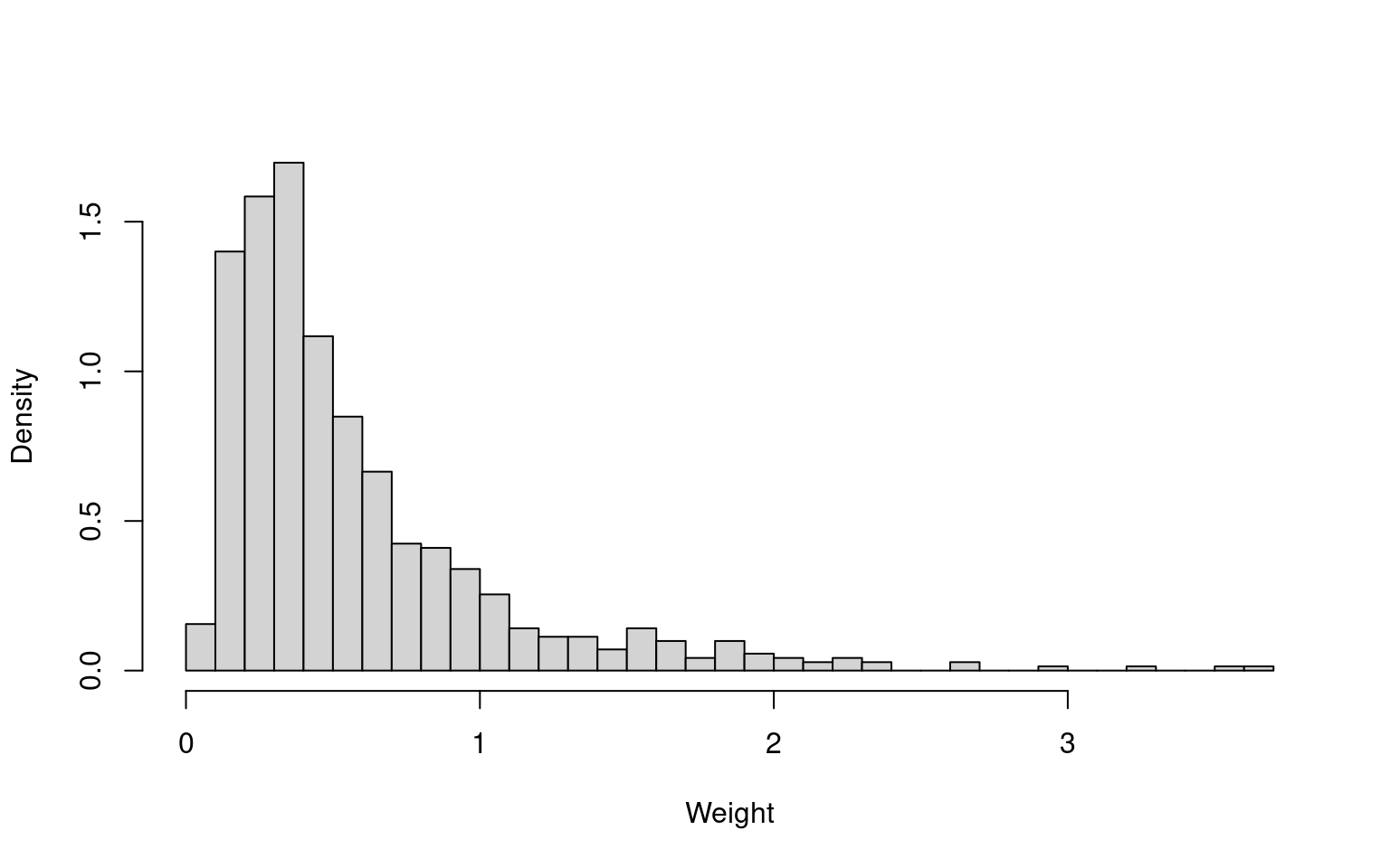
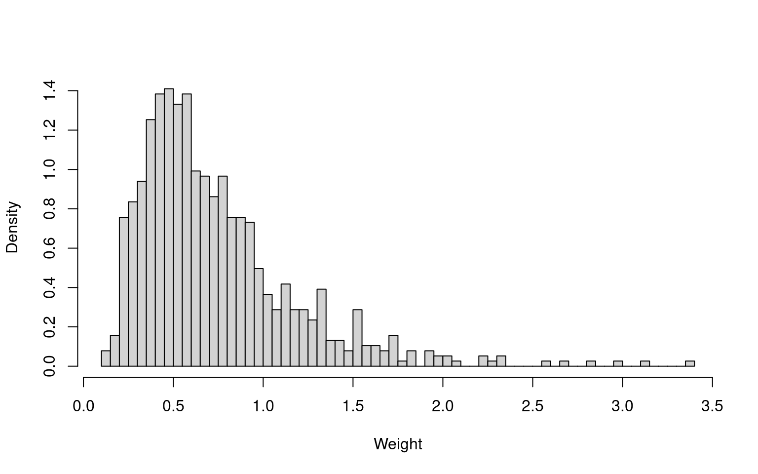
There are no extreme weights, and the effective sample sizes are reasonable in absolute terms. The effective sample sizes are 57.5% (UNCOVER-2) and 73.7% (UNCOVER-3) of the original sample sizes (707 and 766, respectively). The summary statistics of the reweighted samples match the FIXTURE summary statistics (not shown here).
We estimate the treatment effect of ixekizumab vs. etanercept on the probit scale as a probit difference, which can be interpreted as a standardised mean difference, using a simple weighted binomial GLM with probit link function and robust sandwich standard errors within each of the UNCOVER-2 and -3 reweighted samples. We use the sandwich R package for the robust standard errors (Zeileis et al., 2020); alternatively, bootstrapping can be performed. We then combine these estimates with a simple inverse-variance meta-analysis (i.e. fixed effects meta-analysis) to obtain the overall estimate of the ixekizumab vs. etanercept probit difference in the FIXTURE study population.
# Load the sandwich package for robust standard errors
library(sandwich)

# IXE Q2W vs. ETN from UNCOVER-2
fit_uncover2 <- glm(
  cbind(pasi75, 1 - pasi75) ~ trtc,
  data = uncover_ipd[study_ipd == "UNCOVER-2",],
  family = binomial(link = "probit"),
  weights = wt_uncover2
)

# probit difference
d_uncover2 <- coef(fit_uncover2)["trtcIXE_Q2W"]
# sandwich variance
var_uncover2 <- vcovHC(fit_uncover2)["trtcIXE_Q2W", "trtcIXE_Q2W"]

# IXE Q2W vs. ETN from UNCOVER-3
fit_uncover3 <- glm(cbind(pasi75, 1 - pasi75) ~ trtc,
                    data = uncover_ipd[study_ipd == "UNCOVER-3",],
                    family = binomial(link = "probit"),
                    weights = wt_uncover3)

# probit difference
d_uncover3 <- coef(fit_uncover3)[["trtcIXE_Q2W"]]
# sandwich variance
var_uncover3 <- vcovHC(fit_uncover3)["trtcIXE_Q2W", "trtcIXE_Q2W"]

# Obtain inverse-variance weighted estimate and standard error
(d_ETN_IXE <- weighted.mean(c(d_uncover2, d_uncover3),
                            c(1 / var_uncover2, 1 / var_uncover3)))
[1] 1.280599(se_ETN_IXE <- sqrt(1 / sum(1 / var_uncover2, 1 / var_uncover3)))[1] 0.09742977The estimated probit difference and standard error for secukinumab vs. etanercept from the FIXTURE study is
fit_fixture <- glm(cbind(pasi75_r, pasi75_n - pasi75_r) ~ trtc,
    data = fixture_agd,
    family = binomial(link = "probit"))

(d_ETN_SEC <- coef(fit_fixture)[["trtcSEC_300"]])
[1] 0.8937181(se_ETN_SEC <- sqrt(vcov(fit_fixture)["trtcSEC_300", "trtcSEC_300"]))[1] 0.104214Finally, we construct the population-adjusted indirect comparison of ixekizumab vs. secukinumab in the FIXTURE population:
(d_SEC_IXE <- d_ETN_IXE - d_ETN_SEC)[1] 0.3868807(se_SEC_IXE <- sqrt(se_ETN_IXE^2 + se_ETN_SEC^2))[1] 0.1426643Ixekizumab Q2W is estimated to increase the probability of achieving PASI 75 compared to secukinumab 300 mg in the FIXTURE population, with an estimated probit difference of 0.39 (95% CI: 0.11, 0.67).
There are a number of limitations of MAIC, which are apparent in this example. Most importantly, the MAIC estimate is only valid for the FIXTURE study population, but this population is not representative of the selected decision target population (PROSPECT). Furthermore, we have not managed to use all of the available data. Two additional IPD studies and four additional AgD studies were excluded from the MAIC analysis, as they did not include an etanercept arm. MAIC analysis via placebo as a common comparator would have allowed an additional IPD study to be included. Separate MAICs with the different AgD studies as target populations could also have been performed, but all of these would be in different target populations and so would not be comparable, and the IPD would be reused in each analysis. There is no coherent way to synthesise this entire network using MAIC.
Unanchored MAIC analysis
For illustration, we also perform an unanchored MAIC in this network, as if there were no common comparator arms available. The unanchored MAIC code is largely the same as the anchored MAIC code above; the code for data setup and derivation of weights are not repeated here.
After having obtained weights that match the UNCOVER-2 and -3 ixekizumab Q2W arms to the FIXTURE secukinumab 300 mg arm (wt_IXE_uncover2 and wt_IXE_uncover3), these are then used to estimate the average absolute outcomes on ixekizumab Q2W in the FIXTURE population:
# IXE Q2W probability from UNCOVER-2
fit_IXE_uncover2 <- glm(
  cbind(pasi75, 1 - pasi75) ~ 1,
  data = subset(uncover_ipd, studyc == "UNCOVER-2" & trtc == "IXE_Q2W"),
  family = binomial(link = "probit"),
  weights = wt_IXE_uncover2
)

# probit probability
p_IXE_uncover2 <- coef(fit_IXE_uncover2)[["(Intercept)"]]
# sandwich variance
var_IXE_uncover2 <- vcovHC(fit_IXE_uncover2)["(Intercept)", "(Intercept)"]

# IXE Q2W probability from from UNCOVER-3
fit_IXE_uncover3 <- glm(
  cbind(pasi75, 1 - pasi75) ~ 1,
  data = subset(uncover_ipd, studyc == "UNCOVER-3" & trtc == "IXE_Q2W"),
  family = binomial(link = "probit"),
  weights = wt_IXE_uncover3
)

# probit probability
p_IXE_uncover3 <- coef(fit_IXE_uncover3)[["(Intercept)"]]
# sandwich variance
var_IXE_uncover3 <- vcovHC(fit_IXE_uncover3)["(Intercept)", "(Intercept)"]

# Obtain inverse-variance weighted estimate and standard error
(p_IXE <- weighted.mean(c(p_IXE_uncover2, p_IXE_uncover3),
                        c(1 / var_IXE_uncover2, 1 / var_IXE_uncover3)))
[1] 1.397082(se_IXE <- sqrt(1 / sum(1 / var_IXE_uncover2, 1 / var_IXE_uncover3)))[1] 0.07655627The estimated probit event probability and standard error for secukinumab from the FIXTURE study is
fit_SEC_fixture <- glm(cbind(pasi75_r, pasi75_n - pasi75_r) ~ 1,
    data = fixture_agd,
    family = binomial(link = "probit"))

(p_SEC <- coef(fit_SEC_fixture)[["(Intercept)"]])
[1] 0.2669941(se_SEC <- sqrt(vcov(fit_SEC_fixture)["(Intercept)", "(Intercept)"]))[1] 0.04995488Finally, we construct the unanchored population-adjusted indirect comparison of ixekizumab vs. secukinumab in the FIXTURE population:
(d_un_SEC_IXE <- p_IXE - p_SEC) # probit difference[1] 1.130088(se_un_SEC_IXE <- sqrt(se_IXE^2 + se_SEC^2)) # standard error[1] 0.09141308Unanchored MAIC, like the anchored MAIC, estimates that ixekizumab Q2W increases the probability of achieving PASI 75 compared to secukinumab 300 mg in the FIXTURE population. However, the magnitude of the unanchored estimate is very different, and relies on the much stronger assumption that absolute outcomes can be predicted based on the included covariates which is very difficult to justify. Once again, this MAIC estimate is only relevant to the FIXTURE study population, not the PROSPECT target population.
ML-NMR analysis
We now use ML-NMR to analyse this network of evidence, following similar previous analyses (Phillippo et al., 2023, 2020a). ML-NMR coherently synthesises all of the available evidence, allowing comparisons between any pair of treatments in the network, and crucially can produce estimates in any target population of interest for decision making.
ML-NMR models are implemented in the multinma R package (Phillippo, 2024); the following code was run with version 0.7.0. This package was introduced in the context of AgD NMA in Chapter 10. When loading the package we also set the mc.cores option, which enables chains to run in parallel.
library(multinma)
options(mc.cores = parallel::detectCores())
We start by preparing the data. We transform the covariates so binary covariates (psa, prevsys) or percentages (bsa) are given as proportions between 0 and 1, and continuous covariates (weight, durnpso) are approximately unit scaled. The latter step improves computational efficiency when running the model, and also aids interpretation. We furthermore add a variable describing the treatment classes. There are four individuals with missing values for weight, and these are simply excluded.
# IPD studies
pso_ipd <- transform(plaque_psoriasis_ipd,
    # Variable transformations
    bsa = bsa / 100,
    weight = weight / 10,
    durnpso = durnpso / 10,
    prevsys = as.numeric(prevsys),
    psa = as.numeric(psa),
    # Treatment classes
    trtclass =
      ifelse(trtc == "PBO", "Placebo",
      ifelse(trtc %in% c(
        "IXE_Q2W", "IXE_Q4W", "SEC_150", "SEC_300"
      ),  "IL-17 blocker",
      ifelse(trtc == "ETN", "TNFa blocker",
      ifelse(trtc == "UST", "IL-12/23 blocker", NA)))),
    # Check complete cases for covariates of interest
    is_complete = complete.cases(durnpso, prevsys, bsa, weight, psa)
  )

# Only a very small proportion of incomplete rows; we simply remove these
pso_ipd <- subset(pso_ipd, is_complete)

# AgD studies
pso_agd <- transform(plaque_psoriasis_agd,
    # Variable transformations
    bsa_mean = bsa_mean / 100, bsa_sd = bsa_sd / 100,
    weight_mean = weight_mean / 10, weight_sd = weight_sd / 10,
    durnpso_mean = durnpso_mean / 10, durnpso_sd = durnpso_sd / 10,
    prevsys = prevsys / 100,
    psa = psa / 100,
    # Treatment classes
    trtclass =
      ifelse(trtc == "PBO", "Placebo",
        ifelse(trtc %in% c(
          "IXE_Q2W", "IXE_Q4W", "SEC_150", "SEC_300"
        ),  "IL-17 blocker",
        ifelse(trtc == "ETN", "TNFa blocker",
        ifelse(trtc == "UST", "IL-12/23 blocker", NA))))
    )
With the dataset established, we next set up the network. We use the set_ipd() and set_agd_arm() to define the IPD and AgD data sources, which requires specifying the columns that contain the study and treatment indicators, the binary/count outcomes, and the treatment classes. We then use combine_network() to bring the IPD and AgD together into a single network.
pso_net <- combine_network(
  set_ipd(pso_ipd,
    study = studyc,
    trt = trtc,
    r = pasi75,
    trt_class = trtclass),
  set_agd_arm(pso_agd,
    study = studyc,
    trt = trtc,
    r = pasi75_r,
    n = pasi75_n,
    trt_class = trtclass)
)
A network diagram can be created using the plot() function applied to the network object; the following code creates the network diagram in Figure 13.1.
plot(pso_net, weight_nodes = TRUE, weight_edges = TRUE, show_trt_class = TRUE)To incorporate the AgD studies within the ML-NMR model, we need to set up the covariates for numerical integration. This is achieved with the add_integration() function. We specify duration and weight to have Gamma distributions to account for observed skewness in the IPD; body surface area as a proportion is specified to have a logit-Normal distribution; and previous systemic treatment and plaque psoriasis are both binary so are given Bernoulli distributions.
pso_net <- add_integration(pso_net,
  durnpso = distr(qgamma, mean = durnpso_mean, sd = durnpso_sd),
  prevsys = distr(qbern, prob = prevsys),
  bsa = distr(qlogitnorm, mean = bsa_mean, sd = bsa_sd),
  weight = distr(qgamma, mean = weight_mean, sd = weight_sd),
  psa = distr(qbern, prob = psa))
Since we have not specified a covariate correlation matrix, this is calculated automatically from the IPD studies.
We fit a ML-NMR model to this network using the nma() function, specifying a regression model that includes main covariate effects and treatment-covariate interactions using the standard R formula interface. We use a probit link function, and specify that the two-parameter Binomial approximation for the aggregate-level distribution should be used (likelihood = "bernoulli2") (Phillippo et al., 2020a). The shared effect modifier assumption is necessary here to help identify all of the interaction terms in the model, which we introduce by setting treatment-covariate interactions to be equal within each class with class_interactions = "common".
We specify weakly-informative \(N(0, 10^2)\) priors on each parameter using the arguments prefixed by prior_. We narrow the possible range for random initial values with init_r = 0.1 (the default is init_r = 2), since probit models in particular can be challenging to initialise. Using the QR decomposition (QR = TRUE) greatly improves sampling efficiency, as is often the case for regression models.
pso_fit_FE <- nma(pso_net,
                  trt_effects = "fixed",
                  link = "probit",
                  likelihood = "bernoulli2",
                  regression = ~(durnpso + prevsys + bsa + weight + psa)*.trt,
                  class_interactions = "common",
                  prior_intercept = normal(scale = 10),
                  prior_trt = normal(scale = 10),
                  prior_reg = normal(scale = 10),
                  init_r = 0.1,
                  QR = TRUE)
Basic parameter summaries are given by the print() method. Here, for brevity, we only print the individual-level treatment effects d using the pars option.
print(pso_fit_FE, pars = "d")A fixed effects ML-NMR with a bernoulli2 likelihood (probit link).
Regression model: ~(durnpso + prevsys + bsa + weight + psa) * .trt.
Centred covariates at the following overall mean values:
durnpso prevsys bsa weight psa
1.7947485 0.6504375 0.2973544 8.9165934 0.2074278
Inference for Stan model: binomial_2par.
4 chains, each with iter=2000; warmup=1000; thin=1;
post-warmup draws per chain=1000, total post-warmup draws=4000.
mean se_mean sd 2.5% 25% 50% 75% 97.5% n_eff Rhat
d[ETN] 1.61 0 0.08 1.46 1.55 1.61 1.66 1.76 3617 1
d[IXE_Q2W] 2.99 0 0.09 2.83 2.94 2.99 3.05 3.16 4034 1
d[IXE_Q4W] 2.58 0 0.08 2.42 2.52 2.58 2.63 2.74 4280 1
d[SEC_150] 2.24 0 0.09 2.07 2.18 2.25 2.31 2.42 3472 1
d[SEC_300] 2.57 0 0.09 2.40 2.51 2.57 2.63 2.74 3836 1
d[UST] 2.14 0 0.15 1.84 2.03 2.13 2.24 2.44 5159 1
Samples were drawn using NUTS(diag_e) at Thu Jun 5 20:22:39 2025.
For each parameter, n_eff is a crude measure of effective sample size,
and Rhat is the potential scale reduction factor on split chains (at
convergence, Rhat=1).The relative_effects(), predict(), and marginal_effects() functions produce population-average conditional relative treatment effects, predictions of absolute outcomes, and population-average marginal relative treatment effects respectively. Without any target population specified, estimates will be produced for each of the study populations in the network.
relative_effects(pso_fit_FE)
# Average event probabilities
predict(pso_fit_FE, type = "response")
# Population-average marginal effects
marginal_effects(pso_fit_FE, mtype = "link")
# Output not shown
However, we are interested in estimates relevant to the target population represented by the PROSPECT study. To produce estimates for the PROSPECT population, we require a data frame containing the covariate summary information:
prospect_dat <- data.frame(
  studyc = "PROSPECT",
  durnpso = 19.6 / 10, durnpso_sd = 13.5 / 10,
  prevsys = 0.9095,
  bsa = 18.7 / 100, bsa_sd = 18.4 / 100,
  weight = 87.5 / 10, weight_sd = 20.3 / 10,
  psa = 0.202)
Population-average conditional treatment effects for the PROSPECT population can then be obtained by the relative_effects() function with the target population specified as newdata. The argument all_contrasts = TRUE outputs estimates of every pairwise comparison, rather than only the basic relative effects against the reference treatment (placebo). For brevity we do not show these here.
relative_effects(
  pso_fit_FE, newdata = prospect_dat, study = studyc, all_contrasts = TRUE
)
To produce estimates of absolute event probabilities, we need to set up numerical integration for the target population. As when setting up the network, we use the add_integration() function. We choose to use the same forms of the marginal distributions, and use the IPD covariate correlation matrix which is saved in the network object:
prospect_dat <- add_integration(prospect_dat,
  durnpso = distr(qgamma, mean = durnpso, sd = durnpso_sd),
  prevsys = distr(qbern, prob = prevsys),
  bsa = distr(qlogitnorm, mean = bsa, sd = bsa_sd),
  weight = distr(qgamma, mean = weight, sd = weight_sd),
  psa = distr(qbern, prob = psa),
  cor = pso_net$int_cor)
For absolute predictions, we also need a distribution for the baseline risk, either as \(\mu_{(P)}\) or as \(\bar{p}_{k(P)}\)—the latter being much more common. In the PROSPECT population, 1156 out of 1509 individuals on secukinumab 300 mg achieved PASI 75. We use this to place a \(\operatorname{Beta}(1156, 1509-1156)\) distribution on the average response probability \(\bar{p}_{\textrm{SEC 300}(P)}\).
prospect_pred <- predict(pso_fit_FE,
                         type = "response",
                         newdata = prospect_dat,
                         study = studyc,
                         baseline = distr(qbeta, 1156, 1509-1156),
                         baseline_type = "response",
                         baseline_level = "aggregate",
                         baseline_trt = "SEC_300")
prospect_pred
#> ------------------------------------------------------------- Study: PROSPECT ----
#>
#> mean sd 2.5% 25% 50% 75% 97.5% Bulk_ESS Tail_ESS Rhat
#> pred[PROSPECT: PBO] 0.04 0.01 0.02 0.03 0.04 0.04 0.06 4284 3237 1
#> pred[PROSPECT: ETN] 0.44 0.04 0.36 0.41 0.44 0.47 0.52 7005 3384 1
#> pred[PROSPECT: IXE_Q2W] 0.87 0.02 0.83 0.86 0.88 0.89 0.91 5965 3425 1
#> pred[PROSPECT: IXE_Q4W] 0.77 0.03 0.70 0.75 0.77 0.79 0.83 6156 3693 1
#> pred[PROSPECT: SEC_150] 0.66 0.03 0.60 0.64 0.66 0.68 0.71 6374 3528 1
#> pred[PROSPECT: SEC_300] 0.77 0.01 0.74 0.76 0.77 0.77 0.79 4115 3913 1
#> pred[PROSPECT: UST] 0.67 0.06 0.55 0.63 0.67 0.72 0.79 4393 2993 1These can be plotted with the plot() function:
plot(prospect_pred)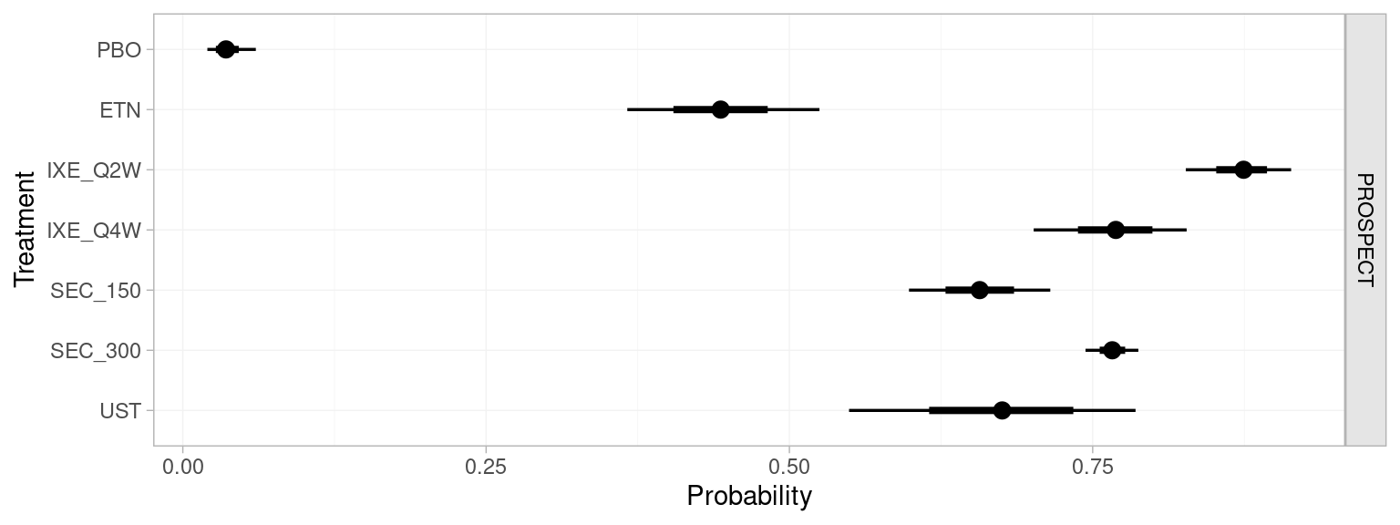
The population-average event probabilities can be used to form population-average marginal treatment effects, following Equation 13.9. The marginal_effects() function produces these marginal treatment effects, and is a wrapper around predict(). Here, for comparison with the MAIC analysis, we produce marginal probit differences; mtype = "link" specifies that the marginal effect should be produced on the link function (i.e. probit) scale.
marginal_effects(pso_fit_FE,
                 mtype = "link",
                 newdata = prospect_dat,
                 study = studyc,
                 baseline = distr(qbeta, 1156, 1509-1156),
                 baseline_type = "response",
                 baseline_level = "aggregate",
                 baseline_trt = "SEC_300",
                 all_contrasts = TRUE)
#> ------------------------------------------------------- Study: PROSPECT ----
#>
#>                                      mean   sd  2.5%   25%   50%   75% 97.5%
#> marg[PROSPECT: ETN vs. PBO]          1.66 0.11  1.44  1.58  1.66  1.73  1.87
#> marg[PROSPECT: IXE_Q2W vs. PBO]      2.95 0.11  2.74  2.88  2.95  3.02  3.16
#> marg[PROSPECT: IXE_Q4W vs. PBO]      2.54 0.10  2.33  2.47  2.54  2.61  2.74
#> marg[PROSPECT: SEC_150 vs. PBO]      2.21 0.12  1.98  2.13  2.21  2.29  2.45
#> marg[PROSPECT: SEC_300 vs. PBO]      2.53 0.12  2.30  2.45  2.53  2.61  2.77
#> marg[PROSPECT: UST vs. PBO]          2.26 0.19  1.90  2.13  2.26  2.39  2.63
#>   ...
#> marg[PROSPECT: SEC_300 vs. IXE_Q2W] -0.42 0.10 -0.62 -0.49 -0.42 -0.36 -0.23
#>   ... output abbreviated ...
ML-NMR provides estimates of all comparisons in the network, not just the focal comparison, in a single coherent analysis. In comparison with the MAIC estimate 0.39 (95% CI: 0.11, 0.67) of ixekizumab Q2W vs. secukinumab 300 mg, the ML-NMR estimated marginal effect is more precise, here primarily because the ML-NMR analysis has used all of the available evidence; more generally, ML-NMR can also be more precise because it allows extrapolation, whereas MAIC does not is sensitive to low effective sample size and extreme weights. Most importantly, these ML-NMR estimates are relevant to the PROSPECT target population, whereas the MAIC estimate is only applicable to the FIXTURE study population.
The multinma package provides features that help to assess the key population adjustment assumptions. These are demonstrated by Phillippo et al. (2023), also using this plaque psoriasis network. Random effects and unrelated mean effects models showed no evidence for residual heterogeneity or inconsistency, which would have indicated the presence of unobserved effect modifiers or other model misspecification. Relaxing the shared effect modifier assumption one covariate at a time showed that this assumption was reasonable; there was some indication that weight might interact differently with the different secukinumab and ixekizumab regimens, but this had little impact on the overall results.
13.5 Methods with no IPD
When no IPD are available, population adjustment methods are currently more limited.
Network meta-interpolation (NMI) has been proposed for scenarios where studies in a connected network report outcomes by subgroups (Harari et al., 2023). The approach “interpolates” estimates within each study to the subgroup mix for a specified target population, before combining these with standard NMA. However, NMI incurs similar biases to plug-in means STC, as the reported study-level treatment effect estimates in trial publications are unlikely to be compatible with the conditional treatment effect estimates required by NMI to perform interpolation unless a linear model with identity link function is used. Moreover, NMI cannot produce estimates of absolute outcomes which are often necessary for decision-making (e.g. as inputs to economic models). Whilst NMI appears promising for certain scenarios, the properties and performance of NMI are not yet fully understood, and simulation studies have not directly investigated bias or adequacy of variance estimation.
Reference prediction and aggregate level matching are approaches to incorporate single-arm studies or disconnected randomised trials (i.e. the unanchored setting) in a larger connected network (Leahy et al., 2019; Thom et al., 2022). Both are based around obtaining a distribution for outcomes on a reference treatment (e.g. placebo) in each of the single-arm studies, against which relative effects can be estimated and synthesised in a NMA model. Reference prediction obtains this distribution with an arm-based random effects pooling of reference treatment arms from trials in the connected network. Aggregate level matching obtains this distribution from a trial in the connected network that is the “best match” in terms of covariate distributions and study design characteristics. Both of these methods rely on the very strong conditional constancy of absolute effects assumption in order to connect the network.
13.6 Discussion
Population adjustment methods are increasingly used in HTA submissions, where it is commonplace for manufacturers to have IPD available from their own studies but only AgD from studies of their competitors. NICE DSU Technical Support Document 18 provides guidance and recommendations on the use of population adjustment methods in a HTA context (Phillippo et al., 2016). At the centre of these recommendations is the explicit need to produce estimates that are relevant to the decision target population. Currently, ML-NMR is the only population adjustment method that can produce estimates in any target population of interest, whereas methods such as MAIC and STC are limited to the population of the AgD study. Moreover, unlike MAIC and STC, ML-NMR can coherently synthesise networks of any size, and in larger networks can allow key assumptions to be assessed or relaxed (Phillippo et al., 2023). In smaller networks like a two-study indirect comparison the shared effect modifier assumption may be required to identify the ML-NMR model, otherwise estimates may similarly be limited to the AgD study population (Phillippo et al., 2020a); this motivates ongoing research that aims to incorporate additional information reported by AgD studies such as subgroup analyses or regression coefficients, to avoid the need for additional assumptions and further improve estimation.
In this chapter we presented an example with binomial outcomes. However, the most common published application of population-adjustment methods is on survival or time-to-event outcomes in oncology, typically analysed with MAIC (Park et al., 2024; Phillippo et al., 2019; Remiro-Azócar et al., 2021a; Serret-Larmande et al., 2023). Phillippo et al. (2024) describe the extension of ML-NMR for survival outcomes, generalising the ML-NMR approach we have outlined in this chapter (Maciel et al., 2024; see also Phillippo, 2019). These methods are also available in the multinma R package, which implements a full range of models and features for survival analysis (Phillippo, 2024).
STC has seen relatively limited uptake in HTA submissions and the wider literature (Phillippo et al., 2019; Remiro-Azócar et al., 2021a; Serret-Larmande et al., 2023). Perhaps a large factor in this is that MAIC is often seen as more straightforward to implement, particularly for survival outcomes. Moreover, it is sometimes said that MAIC has fewer assumptions than STC or other regression-based approaches, since no outcome regression model is explicitly defined. However, we refute this idea: the chosen comparison scale and the covariate moments included in the matching together result in an implicit outcome model that is linear in the covariate moments on the chosen scale (Phillippo et al., 2016). The most common “plug-in means” approach to STC is problematic and biased for non-linear models and for non-collapsible effect measures (Remiro-Azócar et al., 2021a), and previous simulation-based approaches introduce additional uncertainty. The G-computation STC approach proposed by Remiro-Azócar et al. (2022) addresses both of these issues, avoiding aggregation and non-collapsibility biases and appropriately quantifying uncertainty.
Participant weights in a MAIC are typically derived using the method of moments (Signorovitch et al., 2010). Entropy balancing weights have been proposed (Belger et al., 2015), which were later shown to be equivalent to the method of moments (Phillippo et al., 2020b). Other alternative weighting schemes have been proposed, for example those that derive weights to maximise the effective sample size (Jackson et al., 2020). However, the performance of such approaches remains unknown, and these alternative weighting schemes are likely to incur bias as a trade-off for increased effective sample size (Zubizarreta, 2015). Variance estimation for MAIC is typically performed using bootstrapping or robust sandwich estimators (Phillippo et al., 2016; Signorovitch et al., 2010). More recently, Chandler and Proskorovsky (2023) proposed to use conventional variance estimators with the participant weights scaled to match the approximate effective sample size, suggesting that this may provide more accurate variance estimates when overlap is reduced. Previous simulation studies have noted that MAIC is highly sensitive to the level of overlap between populations; when effective sample size is low MAIC can incur substantial bias and variance estimation can be unstable (Phillippo et al., 2020c; Remiro-Azócar et al., 2021a).
There has been much recent discussion over target estimands, and which are appropriate for HTA decision-making (Phillippo et al., 2021; Remiro-Azócar, 2022a, 2022b; Remiro-Azócar et al., 2021b; Russek-Cohen, 2022; Schiel, 2022; Spieker, 2022). Estimates of population-average treatment effects are required for population-level decision-making; however, marginal and conditional population-average effects do not in general coincide, particularly when the effect measure is non-collapsible, e.g. odds ratios or hazard ratios (see Section 13.4.3). Population-average marginal treatment effects quantify the effect of treatment on the expected number of events in the population, and are often considered of primary interest to decision-makers (Remiro-Azócar, 2022a). Population-average conditional treatment effects quantify the average of the individual-level treatment effects in the population. When there is no effect modification, estimates of either estimand will give the same ranking of treatments. However, when effect modification is present the two can result in conflicting rankings: for example, the treatment that achieves the best average event probability overall may be inferior for most individuals in the population; conversely, the treatment that is most effective for each individual on average may result in a worse average event probability overall. This is because effect modification means that there may be no single treatment that is most effective over the entire population. For decisions based on cost-effectiveness, the relevant estimand is the expected net benefit over the population, which in the presence of heterogeneous treatment effects should ideally be accounted for in a suitable economic model such as a discrete event simulation (Welton et al., 2015). The relevant outputs from a population-adjusted analyses are then the inputs to the economic model, which are typically absolute effects on each treatment such as individual, subgroup, or average event probabilities or survival curves. At present, ML-NMR and full-IPD meta-regression are the only population-adjustment approaches that can produce estimates of both conditional and marginal population-average treatment effects as well as the relevant absolute effects for economic modelling, in a chosen population for decision-making.
Unanchored indirect comparisons are prevalent in HTA submissions and the wider literature (Phillippo et al., 2019, 2016; Remiro-Azócar et al., 2021a; Serret-Larmande et al., 2023), despite relying on the very strong assumption that all effect modifiers and prognostic factors in imbalance between studies have been accounted for (conditional constancy of absolute effects, Phillippo et al. (2016)). Unanchored MAIC has been seen to perform well in simulation studies when these stringent assumptions are met, but is otherwise biased (Hatswell et al., 2016). Work is ongoing to extend ML-NMR to incorporate single-arm studies or disconnected networks. More recently there has been interest in so-called “doubly-robust” methods for population adjustment (Park et al., 2024), perhaps sparked by the oft-infeasible, if not near-impossible, strength of the required assumptions for unanchored comparisons. These approaches combine a weighting model with a regression model and promise unbiased estimates if either model is correct, giving the analyst “two chances” to specify a correct model. It has even been suggested that MAIC itself is intrinsically doubly robust (Cheng et al., 2023). Crucially, however, the methods are not doubly-robust to omitted covariates in imbalance between populations (i.e. unobserved confounding), which is precisely the strong assumption of unanchored comparisons with which we are most concerned. A key challenge for unanchored approaches is the development of methods to attempt to validate the very strong assumptions required, and to quantify the potential extent of residual bias due to unobserved confounding. At present these strong assumptions are untestable; the residual bias is unknown and may be substantial. As such, decision makers have justifiably treated unanchored comparisons with strong caution (Phillippo et al., 2019).
Population adjustment analyses are readily implemented in the R ecosystem. Code is available to perform G-computation STC (Remiro-Azócar et al., 2022). MAIC analyses can be performed with the code presented in this chapter, based on the code in TSD 18 (Phillippo et al., 2016), or using a number of R packages (Gregory et al., 2023; hta-pharma, 2024; Lillian Yau, 2022; Young, 2022). A user-friendly suite of tools for performing ML-NMR analyses is available in the multinma R package (Phillippo, 2024), which we have demonstrated in this chapter. This package is also used to perform standard AgD NMA, as we demonstrate in Chapter 10, and full-IPD meta-regression, both of which are special cases of the ML-NMR framework.