1 Introduction to Health Technology Assessment
Anna Heath
The Hospital for Sick Children and University of Toronto, Toronto Canada
Gianluca Baio
University College London, UK
Petros Pechlivanoglou
The Hospital for Sick Children and University of Toronto, Toronto Canada
1.1 Introduction
New technologies in health are being introduced to healthcare systems worldwide in an effort to satisfy societies’ willingness to address disease, improve population quality and length of life. However, given the limited resources available from healthcare systems to cover the cost of those new technologies (in addition to the cost of running the healthcare system in its current form) an assessment needs to be made regarding the value for money for such new technologies.
Health Technology Assessment (or HTA) offers a framework for evaluation of technologies with regards to their comparative effectiveness and safety, their cost-effectiveness but also their ethical and legal implications of their introduction to the healthcare system. Evidence of comparative effectiveness and safety most commonly originate from randomized clinical trials and usually focus on the short to medium term after treatment initiation.
1.2 Basic concepts in cost effectiveness analysis
A certain number of assumptions need to be made when designing a cost-effectiveness analysis for the purpose of HTA. Below we present some of the most important ones:
1.2.1 Time horizon
According to most HTA guidelines, cost-effectiveness analyses (CEA) should capture the totality of the treatment effect across the lifespan of individuals affected by the therapy. That means that for most treatments that are either life saving or have a long period of effect, the CEAs need to have long time horizons. So for example, a new cancer therapy for early breast cancer might be shown to be effective on significantly reducing the risk of recurrence on a clinical trial with a three year follow up, but measuring the full impact of the therapy on an individual would require a lifetime follow up of these breast cancer patients. Since such follow up would be unaffordable and unethical under a clinical trial context, researchers rely on statistical extrapolations and evidence synthesis to estimate such long term impact. Key in such extrapolations are the concepts of survival analysis and decision modeling since they offer approaches to extrapolate beyond any observed follow up under certain assumptions.
1.3 Perspective
Cost effectiveness analysis can be designed to reflect different perspectives depending on who the decision maker is. In cases where the CEA is supporting a governmental body in a publicly funded healthcare system then we usually adopt the healthcare payer perspective. Other times, the patient is the decision maker and the patient perspective is adopted. Finally, the societal perspective takes into consideration the impact of an intervention on society as a whole. That perspective would include both costs and effects that fall within the individual receiving the intervention but also any health or non-health related externalities that the intervention or the disease has on society (e.g increased time off work and productivity losses)
1.4 Discounting
Individuals and societies have historically expressed differences in how much they value rewards or outcomes according to the timing of those rewards. This difference in preference is materialized in HTA through the form of discounting. Discounting accunts for the notions of uncertainty of materializing future benefits (e.g. a disaster), the expectation of larger future earnings and what is referred to as “pure time preference”, the idea that we as humans are inpatient and prefer to receive positive rewards sooner rather than later (and similarly delay negative outcomes).
the rate of annual discounting varies between countries. Most HTA agencies have decided to discount costs and effect outcomes using the same discount rate , with the exception of the Netherlands where differential discounting is implemented. As an example, in Canada the discount rate is 1.5% annually while in the UK is 3.5%.
1.5 Types of Cost-effectiveness analysis
There are multiple forms of economic evaluation including cost-minimization analysis, where effectiveness of the compared therapies are assumed to be equivalent with certainty and only the costs are assumed to vary, cost-benefit analysis, where the health impact of therapies is incorporated in the analysis in the form of monetary impact, and cost-effectiveness analysis were the health impact is captured in a form of natural units (e.g. life years, number of strokes) and the comparison between different therapies is done using an incremental metric such as the incremental cost-effectiveness ratio (ICER) (the mean difference in costs between interventions divided by the mean differnces in effects) .
\[\mbox{ICER} =\frac{ \mbox{E}(\Delta_c)}{\mbox{E}(\Delta_e)}\] A subcategory of cost-effectiveness analysis, where the health impact is captured using a metric called Quality Adjusted Life Years (QALYs), is referred to as cost-utility analysis (CUA). Such QALY based analyses are the most common in the economic evaluation literature Finally, there is cost-consequence analysis where outcomes and disaggregated costs are calculated for each intervention but are not explicitly aggregated in a decision making relevant outcome like the ICER
1.6 Decision modeling in HTA
Health economic decision models aim to compare the costs and effects of different interventions to support decision makers to determine the optimal intervention for widespread implementation (Briggs et al., 2006). These models are the foundation for economic evaluations within health technology assessments (HTAs) that government agencies use to support decision making and maximise population-level health gains, given limited budgets (CADTH, 2019; NICE, 2013). One critical aspect of health economic decision models is that they incorporate evidence from a wide range of sources on the costs and effectiveness of different interventions and evaluate how statistical uncertainty in this evidence impacts decision making (Baio, 2012; Briggs et al., 2006; Willan and Briggs, 2006).
More specifically, health economic decision models compare relevant interventions for a specific health state by assessing their effectiveness, i.e. the clinical benefits, and the associated costs. Costs usually include the cost of acquisition and implementation of the health intervention (e.g. a drug) but may also incorporate societal costs such as those related to number of days off work or social care. As for the clinical benefits, they can be a “hard” measurement (e.g. number of cases averted), but are, most often, considered in terms of Health-related quality of life (HRQoL) measures. Sometimes these estimates originate from indirect methods of eliciting HRQoL. An example is the EQ-5D instrument (Rabin and de Charro, 2001) play a key role. These HRQoL estimates can be combined with estimates of life expectancy to generate a Quality Adjusted Life Years (QALYs, Loomes and McKenzie, 1989), outcome. So QALYs are specifically defined to combine the quantity and the quality of life provided by a given intervention.
Decision models (such as those presented in Chapter 8, Chapter 9 and Chapter 11) often also rely on a natural history model of the disease to estimate the life long impact of intervention, especially for life saving interventions. By combining evidence on the disease natural history, costs and effectiveness, a health economic decision model estimates the population-level average costs and effects for each intervention, based on a set of population-level parameters (Briggs et al., 2006).
The parameters underlying a health economic decision model can be estimated from individual patient level data (as shown in Chapter 5 and Chapter 6), typically using regression modelling (see Section 4.6); alternatively, published sources or expert opinion (Briggs et al., 2012) can be used (see Chapter 10 and Chapter 13). In any case, they are invariably subject to statistical uncertainty (see Chapter 4). The process of probabilistic analysis, sometimes called probabilistic sensitivity analysis (PSA) — although perhaps (parameter) “uncertainty analysis” would be a better term — assesses the impact of this statistical uncertainty on the decision making process (Baio and Dawid, 2011; CADTH, 2019; Department of Health and Ageing, 2008; EUnetHTA, 2014; NICE, 2013). In general, PSA represents the current level of uncertainty in the model parameters using statistical distribution (Claxton et al., 2005), which then induce a distribution for measures of population-average costs and effects for each intervention. This uncertainty distribution for the population-average costs and effects can lead to uncertainty in the optimal decision.
The optimal intervention based on the currently available information is identified by calculating the expected benefit given the costs and effects, with the expectation taken over the uncertainty in the parameters (Claxton, 1999). In theory, this is intervention is optimal irrespective of the associated uncertainty in the underlying evidence (Claxton, 1999). However, it is also important to ask whether the current information is sufficient for decision making or if additional information should be collected before the optimal intervention is selected. These concepts are discussed further in Section 1.8.
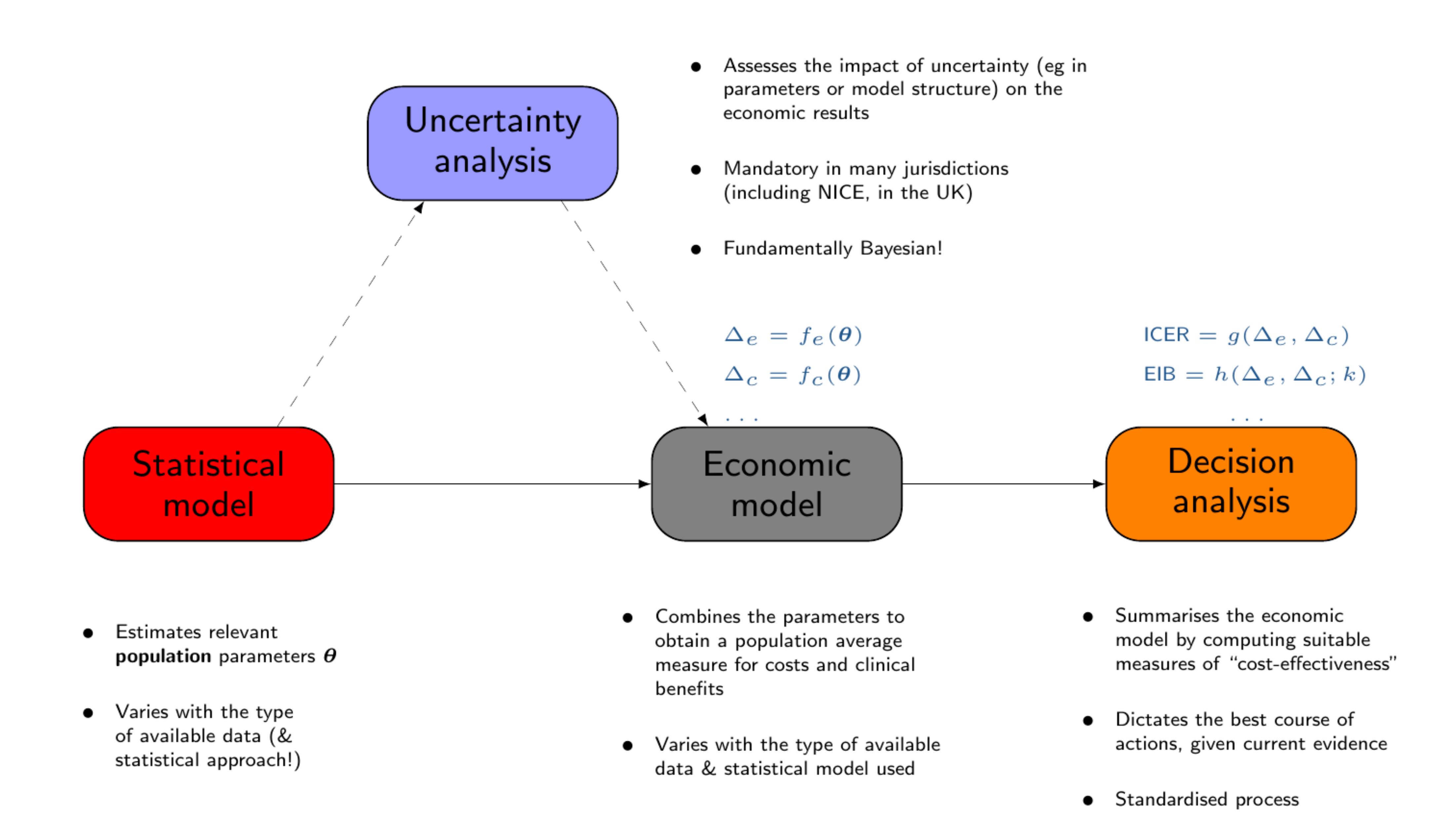
Baio et al. (2017) have described the whole process of economic evaluation in terms of four main “building blocks”, as shown in Figure 1.1.
1.7 Notation and Key Concepts
We assume that we are developing a health economic decision model to determine the optimal intervention among \(D\) alternative options. Interventions are evaluated based on their effectiveness and costs, denoted \((e_d,c_d)\), \(d = 1, \dots, D\). Note that theoretically \(D\) could be arbitrarily large, but is often relatively small, e.g., below 5, except in some settings such as the evaluation of screening interventions (Pokharel et al., 2023). To determine the optimal intervention, the effectiveness and costs can be combined to compute the net monetary benefit (\(nb_d\), Stinnett and Mullahy, 1998), \[nb_d = ke_d - c_d,\] where \(k\) is a willingness to pay (WTP) threshold that represents the amount of money the decision maker is willing to spend to increase the effectiveness measure by one unit. It is also possible to determine the optimal intervention using the net health benefit function (\(nhb_d = e_d - \frac{c_d}{k}\)), but HTA measures are normally calculated on the monetary scale, as this allows us to compare the value of a study against the cost of data collection.
Typically, we consider that the health economic outcomes \((e_d,c_d)\) are subject to individual variability conditional on a set of model parameters \(\bm\theta\), \(p(e_d,c_d\mid\bm\theta)\). The statistical uncertainty in these model parameters (see Chapter 4 for a more detailed description) can then be defined through a probability distribution \(p(\bm\theta)\). This probability distribution should account for all available evidence that is relevant to define the costs and effectiveness for the interventions. Generally, \(p(\bm\theta)\) can be defined by determining either the sampling distribution for the parameters (in a maximum likelihood/frequentist context — see Section 4.4.2 and Section 4.4.3) or directly calculating the Bayesian posterior distribution (see Section 4.4.1) for the parameters. These will almost always be dependent on data that have previously been collected through a range of different study designs including randomised controlled trials, registry data, administrative data and literature reviews. We could explicitly highlight that the distribution for \(\bm\theta\) is dependent on previous data, which we could denote \(\mathcal{D}\), by denoting it \(p(\bm\theta\mid\mathcal{D})\) but, for simplicity, we generally omit to dependence on \(\mathcal{D}\).
Once the relevant uncertainty has been specified in \(p(\bm\theta)\), the ranking of the possible interventions can be obtained by computing the expected net benefit, averaging over both individual variability and parameter uncertainty \[\mathcal{NB}_d = \mbox{E}[nb_d],\] i.e. the expectation here is taken with respect to the joint distribution \(p(nb_d,\bm\theta) = p(nb_d~\mid~\bm\theta)\) \(p(\bm\theta)\). The option \(d\) associated with the maximum expected utility \(\mathcal{NB}^*=\max_d \mathcal{NB}_d\) is deemed to be the most cost-effective, given current evidence. Note that the ranking of the interventions is based on the WTP threshold \(k\) and we usually undertake a sensitivity analysis the explore the cost-effectiveness for different values of \(k\).
1.7.1 Probabilistic Sensitivity Analysis
The intervention associated with the maximum expected utility is theoretically the most cost-effective intervention given the current information. However, uncertainty in the model parameters can lead to uncertainty in the optimal decision. We can explore this decision uncertainty by considering the net benefit as a function of the model parameters, \(\bm\theta\) and only averaging out individual level uncertainty: \[\mbox{NB}_d(\bm\theta) = \mbox{E}[nb_d\mid \bm\theta] \tag{1.1}\]
In Equation 1.1, the expectation is taken with respect to the conditional distribution \(p(e_d,c_d~\mid~\bm\theta)\), termed the known-distribution net benefit (Baio, 2012). Thus, decision making based on current uncertainty is concerned with \(\mathcal{NB}_d\), a deterministic quantity, while the known-distribution net benefit is a \(\mbox{NB}_d(\bm\theta)\) where \(\mbox{E}\left[\mbox{NB}_d(\bm\theta)\right] = \mathcal{NB}_d.\) Crucially, the net benefit incorporates only the uncertainty that could be reduced or eliminated through data collection as the individual-level variability cannot be eliminated.
In health economic decision models, PSA is carried out using a simulation based approach (Andronis et al., 2009; Baio, 2012; Baio and Dawid, 2011). Firstly, \(S\) simulations are obtained from the distribution of the parameters \(p(\bm\theta)\), either through forward-sampling of the uncertainty distribution, or as a by-product of the statistical analysis, e.g. through bootstrap (see for example Section 5.3.3) or MCMC (see Section 5.4 and Section 6.7) methods. The net benefit is then calculated for each simulated vector \(\bm\theta_s\), \(s = 1, \dots, S\). These simulated values for the net benefit \(\mbox{NB}_d(\bm\theta_s)\) then represent simulations from the distribution of the net benefit, accounting for any correlations between the model parameters. These simulations can then be used to explore the impact of parametric uncertainty on decision making.
1.8 Assessing uncertainty and setting research priorities: value of Information
Value of Information (VOI) is a concept from decision theory, the science of making decisions under uncertainty, that formally determines whether additional information is required for decision making (Raiffa and Schlaifer, 1961). VOI measures can also be used to highlight which research designs would efficiently reduce decision uncertainty and provide a cost-effective use of research resources (Ades et al., 2004; Conti and Claxton, 2009).
Overall, VOI encompasses a suite of measures that are defined as the maximum amount a decision maker should be willing to pay to eliminate/reduce parametric uncertainty before making a decision (Willan and Pinto, 2005). We can then compare this maximum with the cost of additional research to collect information to reduce statistical uncertainty in the model parameters to determine whether research should proceed (Heath et al., 2024). Specifically, the cost of research should not exceed the VOI. Furthermore, different research studies can be ranked in terms of their net value (VOI minus study costs) to prioritise studies with a high return on research investment (Conti and Claxton, 2009). Thus, VOI measures form the basis of a comprehensive, principled method for research prioritisation and trial design (Minelli and Baio, 2015).
Despite these advantages, computational issues and a lack of visibility in the clinical community, have largely prevented the widespread implementation of VOI methods (Steuten et al., 2013). Traditionally, the VOI measures with the greatest potential to support research prioritisation and design had to be estimated using computationally costly nested simulation (Ades et al., 2004; Felli and Hazen, 1998). As these simulations required months or even years to obtain an estimate (Heath et al., 2019), VOI could not be used in practice. However, research has developed novel algorithms to overcome these computational barriers and unlock the potential of VOI (Heath et al., 2019, 2018, 2017, 2016; Heath and Baio, 2018; Jalal et al., 2015; Jalal and Alarid-Escudero, 2018; Menzies, 2016; Strong et al., 2015, 2014). These methods have decreased the estimation time for key VOI measures and are implemented in the R package voi to support their implementation (Heath et al., 2024). shiny applications and other more recent graphical interfaces complementing statistical software, such as R are improving the use of VOI in HTA (see Chapter 14).
The overall aim of VOI measures is to quantify the value of collecting additional information before the decision is made. As discussed in Section 1.7, the optimal decision under current information is the intervention that maximises the expected known-distribution net benefit, \[\max_d\mbox{E}_{\bm\theta} \left[\mbox{NB}_d(\bm\theta) \right] = \mathcal{NB}^*.\]
If additional information were collected, it would update the distributions of the model parameters and the known-distribution net benefit. Updating the distribution of the known-distribution net benefit could lead to an alternative optimal intervention, which would have a different value. Thus, the value of collecting additional information is the difference between the net benefit of the new optimal intervention and the net benefit of the intervention that would have been implemented without this updated information, i.e., the net benefit of the current optimal intervention. We consider three key VOI measures that arise by considering different types of information that could be collected to update the known-distribution net benefit.
1.8.1 Expected Value of Perfect Information
The Expected Value of Perfect Information (EVPI) assumes that the additional information specifies the exact value, known as “perfect” information, of every model parameter. If we gather perfect information about all model parameters, \(\bm\theta = \bm\theta'\), then the optimal treatment is known with certainty, as individual level variability has been marginalised out, and its net benefit is equal to \[\max_d\mbox{NB}_d(\bm\theta').\] Thus, the value of learning that \(\bm\theta=\bm\theta'\) is equal to the difference between the value of the optimal intervention when \(\bm\theta=\bm\theta'\) and the value of the optimal intervention under current information when \(\bm\theta=\bm\theta'\). This is because the optimal intervention under current information would be implemented if we made the decision now.
However, we do not know the exact value of \(\bm\theta\) and so we compute the expected value of collecting perfect information by averaging across all possible values of \(\bm\theta\), which is characterised through \(p(\bm\theta)\). Thus, the EVPI is computed as follows: \[\begin{eqnarray*} \mbox{EVPI} & = & \,\mbox{E}_{\bm\theta} \left[\max_d\mbox{NB}_d(\bm\theta) - \mbox{NB}_{d^*}(\bm\theta)\right] \\ & = & \, \mbox{E}_{\bm\theta} \left[\max_d \mbox{NB}_d(\bm\theta)\right] - \max_d \mbox{E}_{\bm\theta}\left[\mbox{NB}_d(\bm\theta)\right], \end{eqnarray*}\] where \(\mbox{E}_{\bm\theta}\) represents the expectation taken with respect to \(p(\bm\theta)\) (Raiffa and Schlaifer, 1961) and \(d^*\) is the optimal intervention under current information.
As EVPI provides the value of learning the exact value of every model parameter, a study that targets a specific set of parameters or does not learn the exact value of a parameters will provide lower value than EVPI. As such, EVPI provides an upper limit for the budget for any study aimed at reducing uncertainty in the model parameters for the specific decision model. If this upper limit is small, then there will be little value in investigating any of the model parameters and the optimal intervention can confidently be selected based on the current information. On the other hand, if the EVPI is high, there may be a study that could generate value for the decision maker. The next two sections discuss VOI measures that can be used to undertake sensitivity analyses, prioritise research studies with substantial value and design studies that will provide a return on investment in research.
1.8.2 Expected Value of Perfect Partial Information
Research studies usually collect information that would reduce uncertainty for a subset of the parameters underpinning the health economic decision model. Thus, it is important to identify which parameters are driving the model uncertainty both as a sensitivity analysis and so research can be targeted towards these parameters. To achieve this, we consider that the parameter vector \(\bm\theta\) can be split into two components \(\bm\theta = (\bm\phi,\bm\psi)\), where \(\bm\phi\) is the sub-vector of parameters of targeted by a proposed study and \(\bm\psi\) are the remaining “nuisance” parameters. The Expected Value of Perfect Partial Information (EVPPI) computes the value of obtaining perfect information about \(\bm\phi\), while remaining uncertain about the remaining parameters \(\bm\psi\) (Felli and Hazen, 1998).
EVPPI can be computed for different parameter subsets \(\bm\phi\) to highlight which subsets have high value and are driving decision uncertainty.
To compute EVPPI, we assume that we are able to learn that \(\bm\phi=\bm\phi'\). Under this condition, the value of the optimal intervention is \[ \max_d \mbox{E}_{\bm\psi\mid\bm\phi'} \left[ \mbox{NB}_d(\bm\phi', \bm\psi) \right], \] where the expectation is taken over the uncertainty in the nuisance parameters. As perfect information about \(\bm\phi\) could improve our knowledge of \(\bm\psi\), this expectation is with respect to the conditional distribution \(p(\bm\psi\mid\bm\phi')\). The value of learning \(\bm\phi = \bm\phi'\) is again the difference between the optimal intervention with the information and the value of the optimal intervention under current evidence.
As the true value of \(\bm\phi\) is not known, EVPPI is calculated as the average value of learning \(\bm\phi\) across all possible values of \(\bm\phi\). The distribution of possible values for \(\bm\phi\) is defined in the PSA through the distribution \(p(\bm\theta)\), \[ \mbox{EVPPI} = \mbox{E}_{\bm\phi} \left[\max_d \mbox{E}_{\bm\psi\mid\bm\phi} \left[\mbox{NB}_d(\bm\phi, \bm\psi)\right]\right] - \max_d \mbox{E}_{\bm\phi,\bm\psi} \left[\mbox{NB}_d(\bm\phi,\bm\psi)\right]. \]
EVPPI is always greater than 0 and less than EVPI as, on average, information cannot make decision making worse. EVPPI represents the maximum amount a decision maker should be willing to pay to reduce uncertainty in the specific subset of model parameters \(\bm\phi\). Thus, if EVPPI is small for a specific subset of model parameters \(\bm\phi\), then future research should not be directed towards to that parameter subset. Conversely, if EVPPI is large, it is likely that research to reduce uncertainty in \(\bm\phi\) would be valuable to the decision maker.
Thus, EVPPI can identify parameter subsets that are driving decision uncertainty and support research prioritisation towards studies that target those parameters. However, as it is rarely possible to obtain perfect information about a model parameter, it is not possible to determine whether a specific study would generate net positive value using EVPPI alone.
1.8.3 Expected Value of Sample Information
To determine the value of a specific study that aims to reduce but not eliminate uncertainty in \(\bm\phi\), we must compute the Expected Value of Sample Information (EVSI) (Ades et al., 2004). In this case, we assume that information will be collected through a research study that gives rise to data \(\bm X\). The notation \(\bm X\) represents any study that collects information to update our model parameters, e.g., a randomised controlled trial of two interventions to estimate relative effectiveness or a retrospective cohort study to estimate disease prevalence. If these data had been collected and realised to a specific dataset \(\bm x\), then the updated PSA distribution for the model parameters would be equal to \(p(\bm\theta\mid\bm x)\). This updated PSA distribution induces a new distribution for the known-distribution net benefit for which the value of the optimal intervention would be \[\max_d \mbox{E}_{\bm\theta\mid\bm x}\left[\mbox{NB}_d(\bm\theta)\right],\] where \(\mbox{E}_{\bm\theta\mid\bm x}\left[\mbox{NB}_d(\bm\theta)\right]\) is the posterior mean of the known-distribution net benefit. The value of collecting \(\bm x\) is then the difference between the values of the updated optimal intervention and the current optimal intervention.
As we do not currently know what data will be collected in the future study, EVSI is computed as the average value of collecting \(\bm X\) over all the possible data sets from the future trial: \[\mbox{EVSI} = \mbox{E}_{\bm X}\left[\max_d \mbox{E}_{(\bm\theta\mid \bm X)} \left[\mbox{NB}_d(\bm\theta)\right]\right] - \max_d \mbox{E} \left[\mbox{NB}_d(\bm\theta)\right].\]
In this equation, the distribution of all possible datasets accounts for both the individual level heterogeneity in the proposed data collected, defined conditional on the model parameters \(p(\bm X\mid\bm\theta)\), and the uncertainty in the model parameters, defined through the PSA distribution \(p(\bm\theta)\) (Heath et al., 2022). This marginal distribution for the future data is \[p(\bm X) = \int_{\bm\Theta} p(\bm X\mid\bm\theta) p(\bm\theta) d\bm\theta.\]
While this distribution is complex to derive, it can be simulated from by simulating a dataset \(\bm X_s\) for each simulated dataset \(\bm\theta_s\) (Heath et al., 2022).
EVSI computes the value of a study that collects data with a specific design. Thus, EVSI should be compared with the cost of collecting the proposed data to determine whether there is net value in undertaking the study. In general, if EVSI is greater than the cost of the study, then it would be valuable to the decision maker. While the study would not be worthwhile if the study cost exceeds EVSI.
1.8.4 Expected Net Benefit of Sampling
While EVSI can be compared to the cost of a study to determine whether it may provide value for a decision maker, there can be a large number of studies that are associated with positive net value. In this case, the study with the largest net value should be prioritized. To support this prioritization, we define the Expected Net Benefit of Sampling (ENBS) as the difference between the population-level EVSI and the study costs.
To define ENBS, we first acknowledge that VOI measures are usually estimated at the individual level. This means that EVPI, EVPPI and EVSI, as presented above, calculate the value of information for each individual who would be affected by the decision. This is because health economic models usually measure the expected individual-level costs and effects for the interventions of interest and VOI is measured directly using these models. Thus, to complete the total net value of perfect information or a specific study, the calculated VOI measures should be multiplied by the number of individuals impacted by the decision population (Thokala et al., 2015).
The total number of people who are impacted by a decision depends on (i) the yearly incidence of the disease \(P\) and (ii) the number of years until the decision is reassessed \(Y\), which we call the decision horizon (Philips et al., 2008). Both of these quantities may be challenging to determine accurately. Firstly, the yearly incidence may change, either increasing or decreasing, and it may be pertinent to include a prevalence “catch-up” cohort in the first year that the decision is implemented. Alternatively, the number of individuals affected by the decision may be capped by implementation considerations such as the number of practitioners who are trained to deliver the intervention.
Secondly, the decision horizon is, by definition, unknown as it is unclear when novel interventions will be available to alter the decision. However, decision horizons of 5, 10 or 20 years are often used for simplicity and sensitivity analyses are performed to account for potential changes in this decision horizon.
Once \(P_y\), the yearly number of individuals affected by the decision, and \(Y\) have been determined, we then typically consider that the value of information for patients who would receive the intervention in the future should also be discounted, in line with standard economic theory (NICE, 2013). Based on these assumptions, the population level EVSI can be estimated as \[\sum_{y = 1}^Y \frac{P_y\mbox{EVSI}}{(1 + r)^y},\] where \(r\) is the discount factor, normally set at 3.5% (NICE, 2013).
Finally, ENBS is then defined as the difference between the population-level EVSI and the cost of the study, \(C_{\text{study}}\). The cost of undertaking the study \(C_{\text{study}}\) can be considered as the sum of three key components (Conti and Claxton, 2009). Firstly, there are fixed costs of research. These costs will be incurred irrespective of the number of individuals enrolled in the study and will include costs such as analyst time to analyse the data, nurse availability to recruit patients and database set up costs. Secondly, there will be per-patient costs including items such as medication, lab testing, research time for follow up pone calls. Finally, we must consider opportunity costs, i.e., the costs of administering the non-optimal treatment to individuals in the study or the cost of delaying decision making until more information is available.
If ENBS is computed for many different designs, it can support research prioritisation and study design. In this case, ENBS for different designs is compared and the study that optimises ENBS is prioritised for funding, provided ENBS is greater than 0. While there is almost an infinite number of study designs that could be considered, ENBS analyses are usually restricted to a small number of key designs and then used to optimise study sample size for each of these designs. More information on the complexity of the ENBS analysis can be found elsewhere (Conti and Claxton, 2009; Heath et al., 2024).
1.8.5 Calculating and using the Value of Information
In general, VOI measures cannot be computed analytically and must be estimated through simulation methods. This is because (i) the known-distribution net benefit is rarely available analytically and is almost always estimated through simulation using a PSA, (ii) it is challenging to calculate the expectation of a maximum, which is required for all VOI measures. As the net benefit underpins all VOI definitions, the PSA simulations for the net benefit will be required for all calculations.
The R package voi (see Chapter 2 for more details on the R language and packages) uses this requirement to develop standardised functions to compute VOI measures. Heath et al. (2024) provide a comprehensive dicussion of the voi package and the specific complexity associated with the computation of VOI measure in practice.
Leaving the technicalities aside and again, redirecting the interested reader to Heath et al. (2024), we concentrate here on what we can do with VOI measures (especially the EVSI and ENBS), once they have been in fact computed. Specifically, ENBS values are based on a (i) the number of individuals who would be affected by the decision each year, (ii) the decision horizon, (iii) the cost of the future trial, (iv) the discount rate, (v) the WTP threshold and (vi) the study sample size. As all these key parameters are often subject to a sensitivity analysis, requiring a range of different graphical displays.
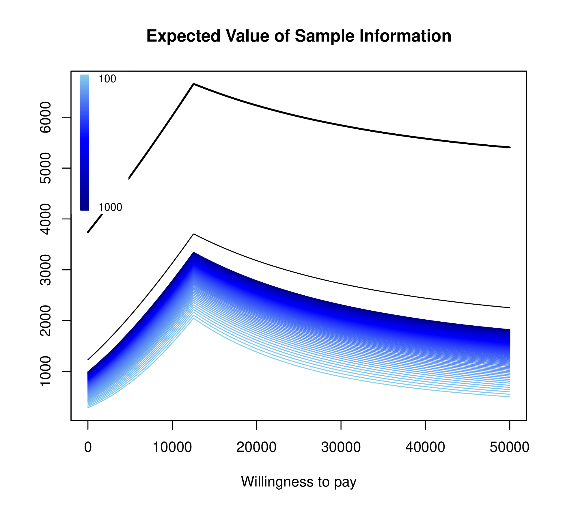
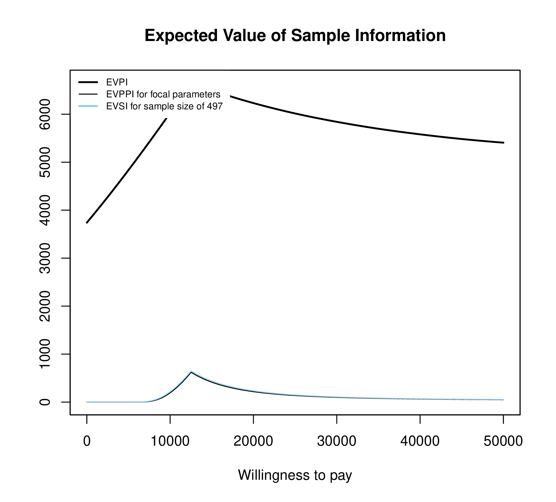
Figure 1.3 plots EVSI, EVPPI and EVPI across WTP values to determine if a proposed study has a positive value for relevant WTP values. The left-hand panel of Figure 1.3 displays EVSI across sample size using darker colours for larger sample sizes and demonstrates how quickly EVSI reaches its maximum value (EVPPI). The right hand side plots EVSI for a specific sample size, which can be easier to read.
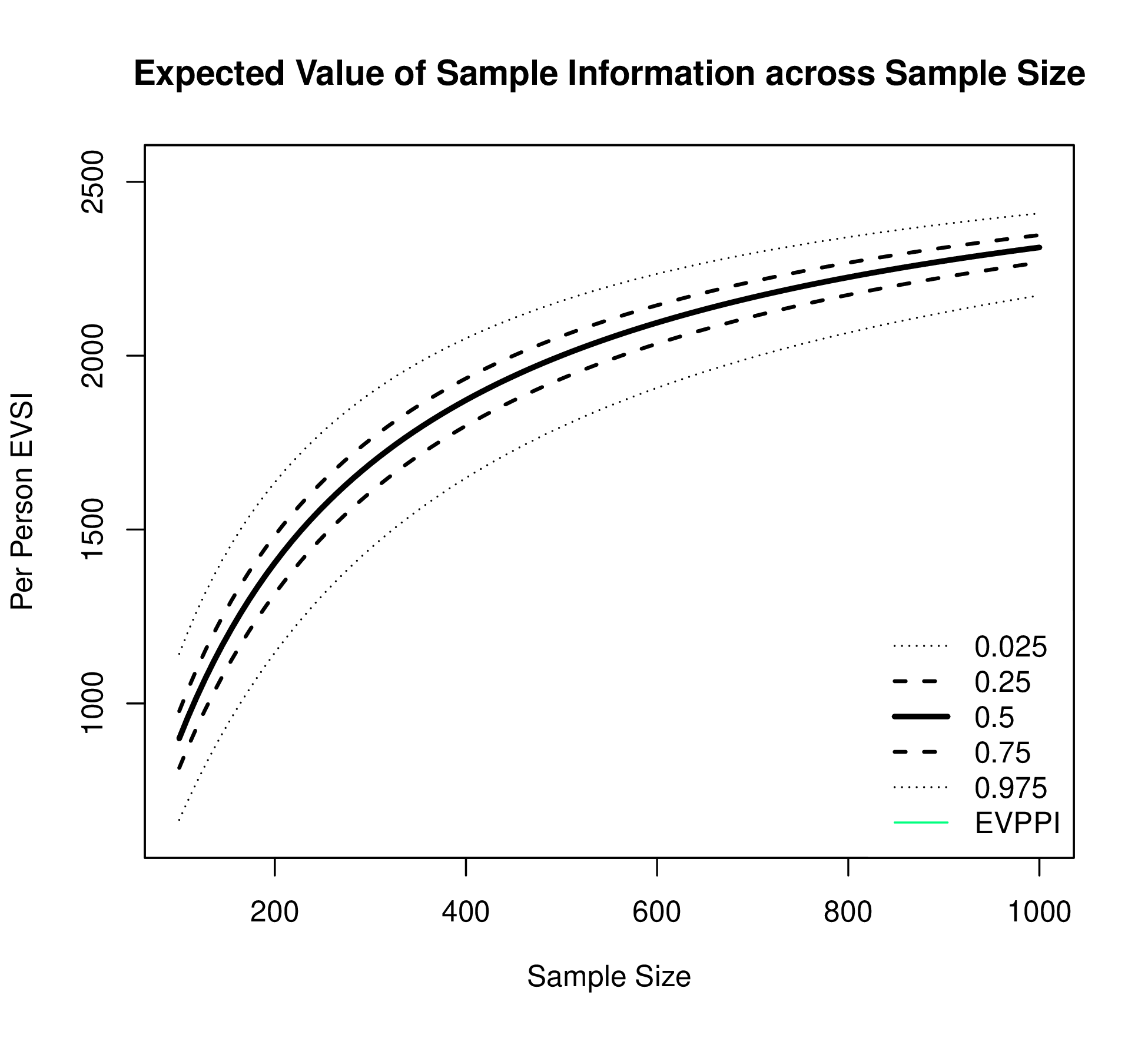
The EVSI can also be plotted against different sample sizes for the proposed study for a fixed WTP threshold (see Figure 1.4 (a)). The EVSI increases across sample size and is bounded above by the EVPPI.
Depending on the method used to compute EVSI, this plot can also display estimation uncertainty for EVSI, which can also support decision making.
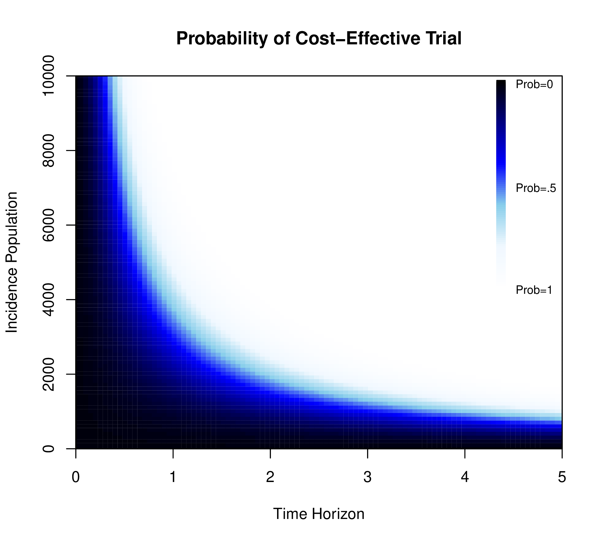
A positive value for ENBS determines whether a specific trial would generate a return on research investment. However, ENBS depends on the yearly incidence and decision horizon, which can then be explored in a sensitivity analysis. Figure 1.4 (b) displays the probability that the ENBS exceeds 0 for different combinations of the yearly incidence population and the decision horizon for a fixed WTP and sample size.
Figure 1.4 (b) varies the yearly incidence populations between 0 and 10,000 and the decision horizon between 0 and 5 years. This demonstrates that the trial is likely to be cost-effective if the decision horizon is greater than 2 and more than 20,000 people are affected by the decision per year.
Finally, the ENBS can be plotted across sample size for a fixed WTP threshold, yearly incidence population and decision horizon. This plot will be similar to Figure 1.4 (a) but will eventually reach an optimal value as the cost of enrolling an additional patient exceeds the additional value generated by including that patient in the trial. More information about calculating and presenting ENBS can be found in Heath et al. (2024).