8 Decision tree models
Nathan Green
University College London, UK
Eline Krijkamp
Erasmus University Rotterdam, Netherlands
Howard Z Thom
University of Bristol, UK
Padraig Dixon
University of Oxford, UK
8.1 Introduction
This is the first of several chapters that introduce the use of R in decision-analytic modelling. This is a tool that involves the structured representation and modelling of outcomes and uncertainties associated with choices over alternative courses of actions. This type of modelling is central to economic evaluation and health technology assessment, in which the fundamental goal is to characterise the relative benefits of different available treatment options, service provisions or other interventions (Briggs et al., 2006; Drummond et al., 2015).
A particular advantage of decision-analytic modelling is that it can be used to extend the scope of questions addressed in other study designs. For example, modelling may be used to combine and synthesise information from multiple information sources, including randomised controlled trials, in order to evaluate the broadest possible range of relevant comparators for a specific intervention.
This chapter demonstrates how R can be used to structure and implement decision trees, a widely used and relatively simple form of decision-analytic modelling. Decision trees are so named because they graphically represent a branching structure, in which different future possibilities are represented by distinct and mutually exclusive “branches”, producing a tree-like shape. Other types of decision-analytic models are described in detail in Chapter 9 and Chapter 11.
8.1.1 Structure of the chapter
The chapter is structured in to two main parts; the first introduces the theory behind decision trees and the second demonstrates this with corresponding R code. In Section 8.2, we provide an overview of the components of a standard decision tree. Section 8.3 introduces a running example that we will use throughout the chapter to illustrate the concepts. Section 8.4 considers more closely the reasons why you would choose to use a decision tree for a particular problem. Section 8.5 gives the mathematical formulation of a decision tree. In particular, Section 8.5.2.1 and Section 8.5.2.2 define the two alternative approaches commonly used to calculate on a decision tree. Section 8.6 explains what we mean by a probabilistic sensitivity analysis (introduced in Section 1.7.1) and how this can be implemented on a decision tree. Section 8.6 extends the example from the previous section to allow a probabilistic sensitivity analysis over model inputs. Section 8.7 provides the R code to implement both of these approaches. Finally, in Section 8.8, Section 8.9 and Section 8.10 we talk about when decision trees should and should not be used, and draw some conclusions.
8.2 Basic components of a decision tree
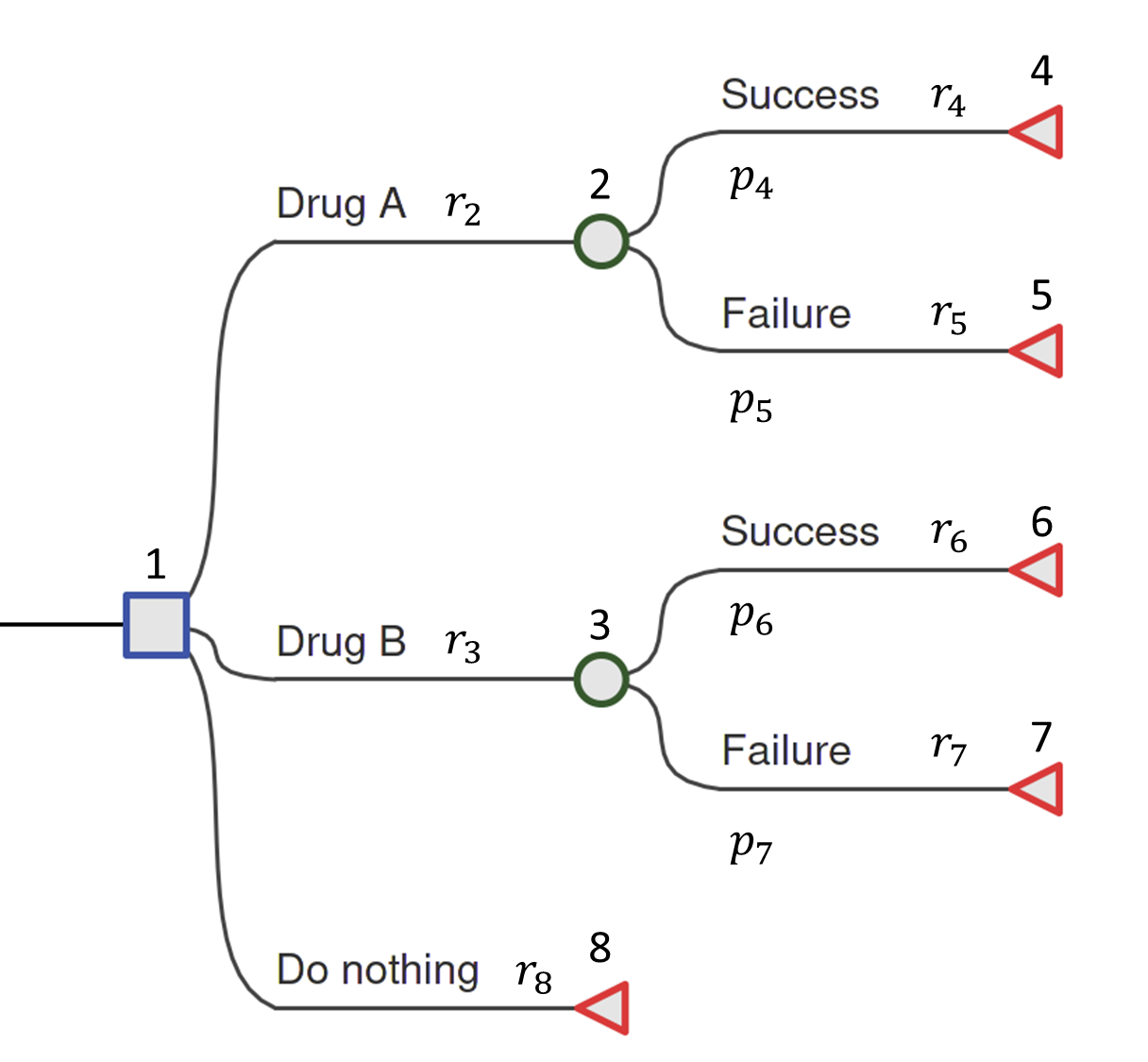
We will introduce the constituent parts of a decision tree using the example shown in Figure 8.1. This is a deliberately simplified model but it still contains all the key features of a decision tree that can then be generalised to more realistic problems. The hypothetical example is of a comparison between two drugs, “Drug A”, “Drug B” and a “Do Nothing” option. This latter option may reflect the possibility that the patient and her doctor will choose not to take either of the drugs, in which case the patient will traverse directly to the terminal node (defined below). Each drug has different costs associated with it and different performance in terms of the chance that the drug is successful at treating the patient.
8.2.1 Types of node
Decision nodes — square
The root of the tree (the leftmost part of the graph) is a decision node and is depicted as a square. From each node a set of branches connect a parent node to its children. This is a one-to-many relationship. In the case of the decision node in Figure 8.1 the branches represent possible drug interventions that may be used. The choice of which branch to traverse is made by the decision-maker, which in different contexts might be a patient, their doctor, or other person(s) responsible for decision-making at different points of the decision-making process. Only one of the (potentially many) alternative options may be chosen.
Chance nodes — circle
Chance nodes are represented by circles. Chance nodes are always associated with an estimated probability since they depict random events. For instance, how a patient responds to a specific drug can either be successful or not successful. However, viewed from the decision-maker’s perspective before the outcome is known, this final outcome for the patient presents an element of unpredictability. Probabilities are used to quantify this uncertainty and reflect the likelihood of specific events described by the decision branches.
Terminal nodes — diamond/triangle
The last node of each pathway is called the leaf or terminal node and is depicted with a diamond or triangle. No further decisions, choices or chances occur after this point. Each terminal node is associated with particular values.
8.2.2 Values
By values we refer generically to the numbers that are attached to the nodes. These are sometimes called rewards in decision-theory and so when not referring to a specific type we will use the letter \(r\). In the HTA context (e.g. a cost-effectiveness analysis), the associated values are usually denoted \(c_i\) and \(e_i\) for the costs and effect measures/health outcomes for each state \(i\), respectively. For example, the outcomes could be measured in quality-adjusted life-years (QALYs; see Section 1.7) over a specified time horizon (e.g. 1 year post-surgical intervention), in quantitative clinical terms such as units of body mass index (BMI) gained, or in disease-specific terms such as the number of headache-free days. Note that the subscript corresponds to the index of the associated node.
8.2.3 Probabilities
This section briefly covers some basic probability theory required for the rest of the chapter — see Chapter 4 for more detailed explanation of some of the mathematics involved. The chance nodes depict random events and so the branches from them have associated probabilities corresponding to the likelihood of traversing to the subsequent node. The probabilities are conditional probabilities, denoted \(p_{ij} = p(x_j \mid x_i)\), which is read as “the probability that event \(x_j\) occurs given event \(x_i\) has already occurred”. Conditional probabilities arise when two or more events are considered. The conditional probability of event A, given event B, is the probability that A occurs given that has B occurred. It is calculated as the probability of both A and B occurring, divided by the probability of B occurring. The joint probability of A and B measures the probability that A and B occur together at the same moment. The marginal probability of A is the individual probability of A, ignoring any value of event B. For a decision tree, using conditional probabilities means that the probability of traversing a given branch is dependent on the fact of being in the previous node. For simplicity, in a decision tree model, since there is only ever a single branch to any node, we shall write \(p_j\). All possible outcomes must be indicated so the probabilities on branches from a chance node must sum to one.
8.2.4 Annotation
Unique node IDs are needed in order to code and calculate on the decision tree model in R. Similarly, branches are labelled to indicate the particular decision (following a decision node) or outcome (following a chance node). The root node is commonly assigned index 1. As described later in Section 8.7, the actual order of labels is not important but it is important that the labels are unique and consistent. However, it is common to number the nodes in ascending order from left to right (from parent to child) and top to bottom (within the same level, between siblings) — see Note 8.1 in Section 8.6 for more details about node numbering.
For example, from Figure 8.1, the decision node has index 1 and its chance child nodes have indexes 2 and 3. The terminal nodes take the remaining indexes \(4,5,6,7,\) and \(8\). For example, the value assigned to the branch from the root node to node 2, which corresponds to selecting Drug A, is denoted \(r_2\).
A final bit of notational convenience, we shall denote the collection of probabilities, cost and effect values as \(\boldsymbol\theta = \{\boldsymbol{p}, \boldsymbol{c}, \boldsymbol{q} \}\). The bold font indicates that these are vectors, which is a collection of numbers. The length of these vectors is equal to the number of nodes in the decision tree.
8.3 A running example
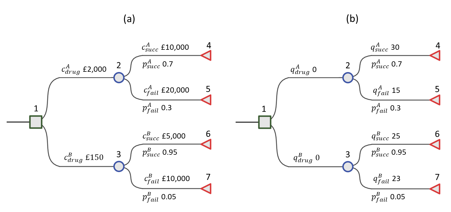
To further clarify matters, we now provide a specific running example. We will continue to return to this example throughout the remainder of the chapter. This is based on the more generic decision tree depicted in Figure 8.1 but without a “Do Nothing” option, which in reality is sometimes not ethical. Firstly, for the health values define the QALYs as \(q_4 = q_{succ}^A = 30\) for Drug A success, \(q_5 = q_{fail}^A = 15\) for Drug A failure, \(q_6 = q_{succ}^B = 25\) for Drug B success and \(q_7 = q_{fail}^B = 23\) for Drug B failure. All other QALYs \(q_i\) are 0. We can think of these as QALYs over a 30 year time horizon without discounting. Because decision trees are often used for short-term decision making, values are often smaller and not discounted. However, if the time horizon is long, then discounting may be appropriate. Similarly to the QALYs, for the cost values assign the cost of Drug A as \(c_2 = c_{drug}^A = £2,000\), the cost of Drug B as \(c_3 = c_{drug}^B = £150\), and the relative success and failure costs as \(c_4 = c_{succ}^A = £10,000\), \(c_5 = c_{fail}^A = £20,000\), \(c_6 = c_{succ}^B = £5,000\), \(c_7 = c_{fail}^B = £10,000\). Finally, the probabilities are \(p_4 = p_{succ}^A = 0.7, p_5 = p_{fail}^A = 0.3, p_6 = p_{succ}^B = 0.95, p_7 = p_{fail}^B = 0.05\). Probabilities are not assigned to the branches coming from the decision node because they are not random, but choices made by the decision-maker.
Figure 8.2 shows the example model populated with the explicit values for costs (a) and QALY gains (b). These numbers can be interpreted to mean that Drug A and B incur fixed and distinct costs for their use of £2,000 and £150, respectively. The subsequent costs, whether Drug A or Drug B are chosen, are different, e.g. due to on-going care. For example, if a decision-maker chooses Drug A and it is unsuccessful then the additional cost is £20,000 but if they had chosen Drug B and that was unsuccessful that would cost £10,000. In terms of the QALY gains health impact, for example, if a decision-maker chooses Drug B and it is successful then this corresponds to 25 QALYs.
8.4 Why use decision trees?
A decision tree is relatively straightforward to construct and analyse, particularly in cases where it can be made to reflect underlying disease natural history and typical treatment outcomes. As a transparent tool to quantify the risks and outcomes associated with different courses of action, it can be easily scrutinised and modified (Caro et al., 2012; Roberts et al., 2012). This makes it straightforward, in most cases, to develop a coherent and tractable model in conjunction with clinicians and non-modellers.
Decision trees represent (clinical) pathways where discrete decisions, costs and outcomes occur in proximal sequence in short time frames, such as diagnostic procedures. In these cases, it may be feasible to represent natural disease history, treatment pathways and relevant outcomes in a decision tree, provided that sufficient data exists to populate all elements of tree. This generally gives rise to a trade-off between detailed representations of clinical pathways and processes and the need for a model to pragmatically but accurately reflect the key variables that are likely to influence optimal decision making.
Decision trees are not well suited to situations where there is a considerable gap between treatment decisions and the realisation of costs and outcomes. Moreover, the influence of time and time dependency is not easily represented in decision trees. At the conclusion of this chapter, we return to examine when and where decision trees should be used and to consider some of the alternatives.
WarningBeware of recurrence
If there is the possibility of returning to a states in the process you wish to represent, such as from a healthy state to illness and then recovery back to a healthy state, then your model needs node recurrence (including staying in state), and it may be better to consider a more compact alternative, such as a Markov model (see Chapter 9). It is possible to simply duplicate repeated structure in a decision tree but a large number of (duplicated) nodes can lead to an unwieldy tree. For example, see Figure 8.8.
8.5 Calculations on a decision tree
As mentioned, the probabilities along each branch of the decision tree are conditional probabilities, \(p(x_j \mid x_i)\). This is important to note for the calculations of expected costs and expected health impacts. As a reminder refer back to Chapter 4 for more detailed definitions.
8.5.1 Probabilities of moving along branches
The complete set of all possible outcomes in the model is represented by the set of terminal nodes on the right-hand side of the decision tree. Figure 8.3 shows schematically all of the possible pathways through the decision tree for our motivating example.
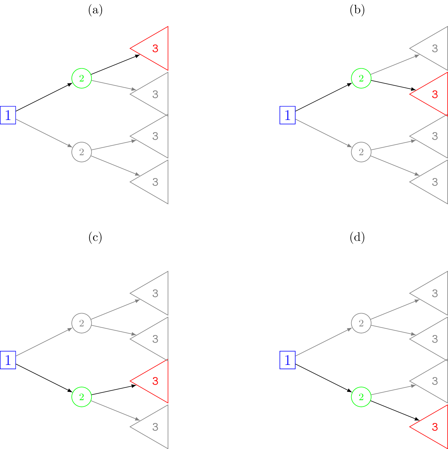
We can think of a unique pathway from the root node, going step-by-step from left to right, until finally reaching a terminal node. At each chance node along the way one of the possible outcomes can occur. By chaining the conditional probabilities for a given pathway we can obtain the total or joint probability of reaching a terminal node. Each pathway through the tree is a mutually exclusive sequence of events. If we define \(x\) to be the event variable then consider one such pathway through the tree with length of \(n\) nodes as \[ x_{[1]} \rightarrow x_{[2]} \rightarrow x_{[3]} \rightarrow \cdots \rightarrow x_{[n]}, \] where \(x_{[1]} = x_1\) is the root node (often the decision node), \(x_{[n]}\) is a terminal node and the square brackets indicate that this is the \(i\)-th ordered nodes in the sequence. By the product rule (recall Equation 4.2), the joint probability of this path can be factorised as \[ p(x_{[1]}, x_{[2]}, \ldots, x_{[n]}) = p(x_{[2]} \mid x_{[1]}) p(x_{[3]} \mid x_{[2]}) \cdots p(x_{[n]} \mid x_{[n - 1]}) = \prod_{i=1}^{n - 1} p(x_{[i + 1]} \mid x_{[i]}). \]
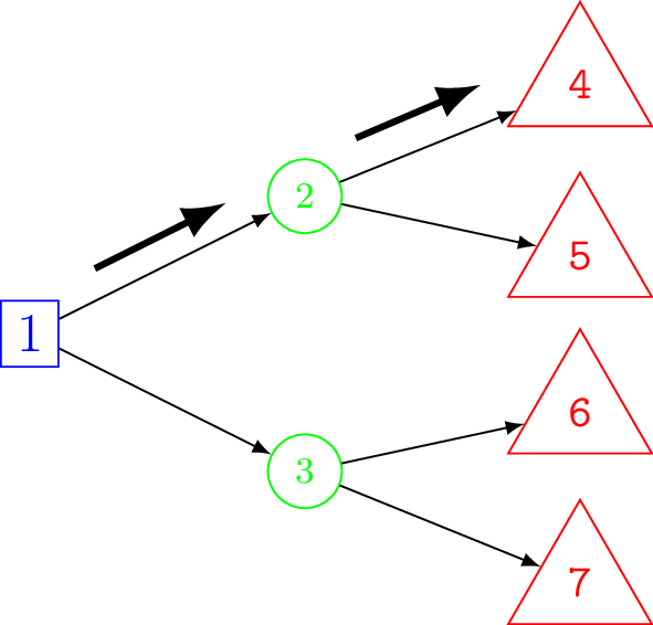
For example, for the decision tree in Figure 8.1, one possible pathway through the tree is selecting Drug A and observing success. That is, \(x_{[2]}\) is the decision to use Drug A and \(x_{[3]}\) is the event of a successful treatment. The probability of traversing this pathway is \[ p(\mbox{Drug A}, \mbox{Success}) = p(\mbox{Success} \mid \mbox{Drug A}) p(\mbox{Drug A}) = p(\mbox{Success} \mid \mbox{Drug A}) = p^A_{succ} = 0.7, \] i.e. just the conditional probability of success for Drug A (because the choice of Drug A is deterministic so is known with probability 1). This pathway corresponds to that shown in Figure 8.8 (a). For the above pathway, the corresponding cost and effects are \(\boldsymbol{c} = \left( c_{[1]}, c_{[2]}, \ldots, c_{[n]} \right)\) and \(\boldsymbol{q} = \left( q_{[1]}, q_{[2]}, \ldots, q_{[n]} \right)\).
8.5.2 How to calculate expected values
Finding the optimal decision using a decision tree is called solving the decision tree and to do so we first need to calculate the expected values of each decision. There are two alternative approaches used for calculating the expected cost and effectiveness on a decision tree. Figure 8.4 shows a schematic of these two approaches, a backwards and forwards approach of computation.

Folding back (backwards) computation
The first approach is to work backwards, usually called folding back (Briggs et al., 2006), because the child nodes are folded up or collapsed, so that a chance node is now represented by its expected value. In other words, folding back takes a weighted average of the total values of the child nodes of a parent chance node where the weights are the probability of traversing each branch to the child nodes. Note that the term folding back is sometimes reserved specifically for the process of removing less optimal alternatives when working backward with the decision tree and the more general process including averaging called rolling back (Hunink et al., 2014). However, we will use the term folding back to refer to the general process of working backwards.
Starting at the right-most terminal nodes the expected values (e.g. cost or QALYs) at each chance node are calculate in turn and the tree can thus be folded back all the way to the decision node. This is an example of something called a recursive function which is a function that calls itself during its execution. A well-known example is when calculating the Fibonacci series.
This approach is part of a whole field of stochastic optimisation in applied probability called Markov Decision Processes (MDP), which provides a general mathematical framework for modelling decisions under uncertainty (Howard, 1960). The formulation presented here is a special case of the more general MDP equations, where the alternative interventions are usually represented as separate trees.
Recall the conditional probabilities \(p_{ij} = p(x_j \mid x_i)\); then the expected value at node \(i\) is \[ \mbox{E}[V_i] = \left\{ \begin{array}{lcl} r_i & \mbox{ if } & i \in \mathcal{N}_{term}\\ r_i + \sum_{j \in ch(i)} p_{ij} \mbox{E}[V_j] & & \mbox{otherwise,} \end{array} \right. \tag{8.1}\] where the operator \(\mbox{E}[\cdot]\) indicates the expected or weighted average of the values, \(r_i\) is the (unit) value at node \(i\) and \(V_i\) is the total value at a node which consists of \(r_i\) and the values of the child nodes along a trajectory. We do not know in advance which pathway will be taken and so \(V_i\) is a random variable, and we must take the expectation over all possible pathways. Adopting notation used in Bayesian networks and graphical models, the set of child nodes, i.e. possible traversals, from node \(i\) is defined as \(ch(i)\). Practically, this summation could be taken over all nodes and those not in \(ch(i)\) assigned probability 0. Finally, \(\mathcal{N}_{term}\) is the set of all terminal node IDs. Note that at a terminal node the expected value is simply the value at that node.
An advantage of using this method is that total expected values can be obtained at each node and so if there are multiple decision nodes, not just at the root of the tree, then the recursive approach can fold-back sub-trees.
In our example decision tree in Figure 8.2, folding back to the decision node takes only a single step. For \(d =\) Drug A or Drug B, the equations for the expected costs and QALYs respectively are \(c_{drug}^d + p_{succ}^d c_{succ}^d + p_{fail}^d c_{fail}^d\), and \(p_{succ}^d q_{succ}^d + p_{fail}^d q_{fail}^d\).
Plugging in the values then the expected cost for Drug A is \(\hbox{£}15,000 = \hbox{£}2,000 + 0.7 \times \hbox{£}10,000 + 0.3 \times \hbox{£}20,000\) and Drug B is \(\hbox{£}5,400 = \hbox{£}150 + 0.95 \times \hbox{£}5,000 + 0.05 \times \hbox{£}10,000\). The expected QALYs for Drug A are 25.5 = 0.7 \(\times\) 30 + 0.3 \(\times\) 15 and Drug B are 24.9 = 0.95 \(\times\) 25 + 0.05 \(\times\) 23.
Forward computation
The second approach is in contrast to the folding back approach and may be more intuitive. It is called folding forward or, simply, forward computation (Frank et al., 1993). It involves first calculating the total health and costs, and joint probability along all of the distinct pathways of the tree corresponding to a decision. That is, imagine that we were to terminate at a particular node. Then what would be the sum of the costs and joint probability associated with reaching there. The total costs and health values are called the payoffs. The weighted average of the costs or health values give the expected value at the decision node. Formally, this can be written as \[ \mbox{E}[V] = \sum_{j=1}^{m} r^*_{j} p^*_{j} \tag{8.2}\] where \(r^*_j = r_{[1]} + r_{[2]} + \cdots + r_{[n_j]}\) is the sum total of the values (i.e. cost or health impact) along each pathway, \(j = 1, \ldots, m\) of length \(n_j\), and \(p^*_j\) is the associated joint probabilities of traversing the unique path as defined in Section 8.5.1. In our running example, all of the possible pathways are shown in Figure 8.3. There are \(j = 4\) pathways and all have length \(n_j = 2\).
NoteRecursively Calculating \(r^*\) and \(p^*\)
For a more algorithmic approach, in comparison with the recursive backwards equation when folding back, \(r^*_j\) and \(p^*_j\) may be calculated by the following. \[ r^*_i = \left\{ \begin{array}{lcl} r_1 & \mbox{ if } & i = 1 \\ r_i + r^*_{pa(i)} & & \mbox{otherwise} \end{array} \right. , \quad p^*_i = \left\{ \begin{array}{lcl} 1 & \mbox{ if } & i = 1 \\ p_i \times p^*_{pa(i)} & & \mbox{otherwise} \end{array} \right. \tag{8.3}\] where \(pa(i)\) is the set of parent nodes of node \(i\), which in our special case on a decision tree is just a single node. Intuitively, this equation will step along the decision tree one node at a time from right to left (from a terminal node) until reaching the root node \(i=1\). The strength of this formulation is in the implementation; the distinct pathways do not need to be defined in advance of the calculation, only the relationship between neighbouring nodes. Clearly, the key difference between these two equations is that at each step the values are either summed or multiplied.
Back to the decision tree in Figure 8.1, if the decision-maker chooses Drug A then the joint probabilities for success and failure are simply the conditional probabilities and the payoff costs are \(£12,000 = £2,000 + £10,000\) and \(£22,000 = £2,000 + £20,000\), respectively. Using Equation 8.2, this gives the expected cost for Drug A as \(£15,000 = 0.7 \times £12,000 + 0.3 \times £22,000\). In this simple example, the backwards and forward calculations are very similar and the decisions made under each approach are identical. The difference is that for the forward computation the drug cost is included in the payoff cost before taking the weighted average. In general, the computation using both approaches may not be so similar.
Table 8.1 gives the payoff table for the example decision tree model. This is a convenient way to show all of the \(r^*\) health and cost payoffs from a decision tree.
| Cost (£) | QALYs | |||
|---|---|---|---|---|
| Drug A | Drug B | Drug A | Drug B | |
| Success | 12000 | 5150 | 30 | 25 |
| Failure | 22000 | 10150 | 15 | 23 |
8.5.3 Optimal decisions
Using the expected costs and effects for different decisions calculated at the decision nodes in the decision tree (e.g. in our example this is the decision between Drug A or Drug B at the root node) we can determine the optimal course of action to obtain the maximum expected benefit in the usual way for Health Technology Assessment (HTA).
Table 8.2 gives outputs of the cost-effectiveness analysis for our example decision tree model in the standard results format. The incremental mean QALYs and cost are denoted by \(\Delta_q := \mbox{E}(q\mid \theta^A) - \mbox{E}(q\mid \theta^B)\) and \(\Delta_c := \mbox{E}(c\mid \theta^A) - \mbox{E}(c\mid \theta^B)\). In our example, we assume that Drug B is the reference or “standard” drug (called the “comparator” in a population, intervention, comparator and outcomes (PICO) framework) and Drug A is the newer (“intervention”) drug. The common utility functions used for decision making, Incremental Cost-Effectiveness Ratio (ICER) and Incremental Net Monetary Benefit (INMB), are also provided. It is clear for a £20,000 per QALY willingness to pay threshold that Drug A is preferred. As an extension to our example decision tree with only a single decision node, the decision tree may contain multiple decision nodes. This is less common in health technology assessment. In this case, once the best choice has been identified at a decision node, all of the other options can be eliminated for further consideration. This is referred to as pruning the tree. The process would continue from right to left, calculating expected values and pruning at each decision node until the root node is reached (Hunink et al., 2014).
| Cost (£) | QALYs | $\Delta_c$ (£) | $\Delta_q$ QALYs | ICER (£/QALY) | INMB (£) | |
|---|---|---|---|---|---|---|
| Drug A | 15000 | 25.5 | 9600 | 0.6 | 16000 | 2400 |
| Drug B | 5400 | 24.9 |
Note 8.1: Trees in Computer Science
In the field of computer science, calculating on trees is a well-studied problem and there are many algorithms for doing so (Cormen et al., 2001). In particular, related to our folding-back approach, a breadth-first search is the process of inspecting every node on a level starting at the root of the tree and then move to the next level. Similarly, in comparison to the folding forward approach, a depth-first search is a process which searches deep into a branch and does not move to the next one until the terminal node has been reached. Each approach has unique characteristics, including how the nodes are numbered, but the process for each one is almost exactly the same. The only difference in their approach is how they store in memory the nodes that need to be searched at each step.
8.6 Probabilistic Sensitivity Analysis (PSA)
So far we have made no consideration for uncertainty. However, from a policy perspective in particular, it is important to account for any uncertainty in the modelling process (Briggs et al., 2012; Thom et al., 2022; Welton et al., 2012). The model should provide measures of uncertainty around point estimates to better inform decision making. Uncertainties can be incorporated into the model for the probabilities, health values, and costs. In the literature, uncertainty is often divided into three forms. These are stochastic (first-order) uncertainty which is distinguished from parameter (second-order) uncertainty. Further, there may be structural uncertainty but we will not be considering that here — see Section 1.7.1, Baio (2012) and Briggs et al. (2012) for further details.
Stochastic uncertainty is the uncertainty around a realisation at an individual level. This can be thought of as corresponding to the unexplained error term in a regression model. Parameter uncertainty is that uncertainty about the model input parameters, such as the cost of a drug or the QALY detriment due to adverse effects of a treatment. This is due to the fact that we may only have a sample from a population and this may not be the particular target population of interest. In the main, cost-effectiveness analysis and HTA are primarily concerned with parameter uncertainty because the focus is on population averages, rather than an individual. In particular, although they can used for microsimulation, a decision tree is often employed as a type of cohort model and as such is not concerned with individual level uncertainty.
There are different ways of performing a sensitivity analysis. A deterministic sensitivity analysis (DSA) varies parameter values manually to test the sensitivity of the model outputs to specific (sets of) parameters. Alternatively, a probabilistic sensitivity analysis (PSA) varies all parameters simultaneously. These are sampled from a (joint) probability distribution, which may be derived from summary statistics (e.g. from literature) or a Bayesian posterior distribution. PSA of decision trees is often preferred to deterministic analysis since it is almost always more informative to vary all parameters simultaneously in sensitivity analysis. Different HTA jurisdictions have (slightly) different requirements, with some making it a formal requirement (Australian Government Department of Health and Aged Care, 2023; CADTH, 2019; HIQA, 2019; NICE, 2013; ZiN, 2024).
More formally, when doing PSA in health economics, for each of a sequence of iterations \(s = 1, \ldots, S\), a value of all random input values \(\theta_{(s)}\) is simulated from the distribution \(p(\theta)\). The decision tree model is then run with these values and a distribution of expected incremental costs and health values calculated (Baio and Dawid, 2011). That is, we obtain a sample of pairs \((\Delta_q^{(s)}, \Delta_c^{(s)})\) where \(\Delta_q^{(s)} := \mbox{E}(q\mid \theta^A_{(s)}) - \mbox{E}(q\mid \theta^B_{(s)})\) and \(\Delta_c^{(s)} := \mbox{E}(c\mid \theta^A_{(s)}) - \mbox{E}(c\mid \theta^B_{(s)})\).
8.7 Implementing decision trees in R
In this section, we will show how to perform a cost-effectiveness analysis of the model in Figure 8.1 using base R. We will first implement the forward model approach before demonstrating an example implementation of the folding back method. The simpler point value case and then PSA versions of both approaches will also be given.
Note that the purpose of this section is to show how to implement a simplified decision tree from scratch to aid understanding of the theory and be general to other problems. Alternatively, there are several excellent existing packages for working with trees in R which could be adopted. The R package igraph (Csardi and Nepusz, 2006) is a powerful tool for working with graphs and trees and has many functions for calculating on them.
8.7.1 Forward computation
Firstly, the number of treatments is defined, and names assigned.
tx_names <- c("Drug A", "Drug B")  # treatment names
n_treat <- length(tx_names)        # number of treatments
The costs, QALYs and probabilities of movements between nodes will need to be assigned, so the code creates some empty containers to fill in once calculations are performed. In R, these can be represented with NA (not available). The R language treats NAs specially, so they cannot be accidentally confused with numbers or characters. The use of c_*, q_* and p_* in the code corresponds to the costs, QALYs and probabilities, respectively. Note that we could have placed all costs, QALYs and probabilities in a single array object, rather than assigning them to separate variables. There is no “right” way of doing this and our choice is reasonable given the structure of the decision tree and ease of exposition.
# define value arrays
c_success <- c_failure <- setNames(rep(NA, times = n_treat), tx_names)
q_success <- q_failure <- setNames(rep(NA, times = n_treat), tx_names)
p_success <- p_failure <- setNames(rep(NA, times = n_treat), tx_names)
For example, the costs of a successful drug is
c_successDrug A Drug B
NA NA The rep() function repeats NA a set number of times, in this case n_treat. setNames() labels each of the entries with the treatment names.
Next, we will populate the information about the decision tree from Section 8.3 into the newly created NA “blank spaces”. The vector can be indexed using the drug names. For example, in this case Drug A is the first entry. We could have used numbers to index and access each intervention, but in this model with just two treatments it is convenient to use the drug names. This make the code easier to read and understand. It is also a more robust way to assign and access values because it does not depend on the ordering of values. The QALY values are assigned as follows.
# assign QALY values
q_success["Drug A"] <- 30; q_failure["Drug A"] <- 15
q_success["Drug B"] <- 25; q_failure["Drug B"] <- 23
For costs, we proceed in a similar fashion. Note that there are additional initial costs, c_drug, as well as lifetime costs for each drug.
# assign cost values
c_drug <- c("Drug A" = 2000, "Drug B" = 150)
c_success["Drug A"] <- 10000; c_failure["Drug A"] <- 20000
c_success["Drug B"] <- 5000; c_failure["Drug B"] <- 10000
The probabilities of successful and unsuccessful outcomes from the use of each drug are now defined. As success and failure are mutually exclusive, we may calculate the probability of failure as one minus the probability of success.
# assign probabilities
p_success["Drug A"] <- 0.7
p_failure["Drug A"] <- 1 - p_success["Drug A"]
p_success["Drug B"] <- 0.95
p_failure["Drug B"] <- 1 - p_success["Drug B"]
In the same way as we created empty containers of NAs previously, we will create objects for the expected total and incremental cost and QALYs.
c_total <- q_total <- setNames(rep(NA, n_treat), tx_names)
c_incr  <- q_incr  <- setNames(rep(NA, n_treat), tx_names)
This is the final step of the general model preparation. We can now perform the forward calculation on the decision tree to obtain the total costs and total QALYs estimates for each choice of drug. Referring back to the analysis in Section 8.5.2.2, the expected total cost (QALYs) is the sum of products of the total costs (QALYs) and joint probabilities along each distinct traversal along the decision tree. We denote \(c^*\), \(q^*\) and \(p^*\) with c_star, q_star and p_star, respectively. The values of c_star and q_star correspond to the values in the payoff table in Table 8.1. Note that the q_star calculation only contains a single term because there is no QALY detriment to the drug decision.
# path joint probabilities
p_star <- rbind(p_success, p_failure)

# path total costs
c_star <- cbind(c_drug + c_success, c_drug + c_failure)

# path total QALYs
q_star <- cbind(q_success, q_failure)
From Equation 8.2, we can explicitly take the sum of each product term to obtain the total expected values.
# expected values for Drug A
sum(c_star["Drug A", ]*p_star[, "Drug A"])
[1] 15000sum(q_star["Drug A", ]*p_star[, "Drug A"])[1] 25.5# expected values for Drug B
sum(c_star["Drug B", ]*p_star[, "Drug B"])[1] 5400sum(q_star["Drug B", ]*p_star[, "Drug B"])[1] 24.9However, we may also make use of R’s matrix multiplication feature for a more succinct solution. The %*% in-fix operator calculates the dot product matrix of the two matrices to the left and right of it. In our case, we are only interested in the matching columns and rows for Drug A or B and so we drop the off-diagonal elements in the output using the diag command.
diag(c_star %*% p_star)Drug A Drug B
15000 5400 diag(q_star %*% p_star)Drug A Drug B
25.5 24.9 In fact, it is straightforward in this particular problem to calculate the expected total costs and QALYs for each drug by writing out the equations in full explicitly. The expected costs for each drug are calculated in a single step using R’s memberwise vector arithmetic. Notice that we take the c_drug term outside of the brackets because it is present in both pathways and so its probability sums to one. The calculation of total QALYs for each drug choice is similar.
c_total <- c_drug + (p_success*c_success + p_failure*c_failure)
q_total <- p_success*q_success + p_failure*q_failure
To calculate incremental cost and QALYs, recall that we assume Drug B is the reference and Drug A is the comparator. Subtract the values of total cost and total QALYs of Drug B from Drug A.
c_incr <- c_total["Drug A"] - c_total["Drug B"]
q_incr <- q_total["Drug A"] - q_total["Drug B"]
The incremental cost-effectiveness ratio (ICER) and incremental net monetary benefit (INMB) can now be calculated as the ratio of incremental costs to incremental QALYs, and difference between health benefit and cost incurred on the monetary scale, respectively.
k <- 20000 # willingness to pay threshold (GBP)
icer <- c_incr/q_incr
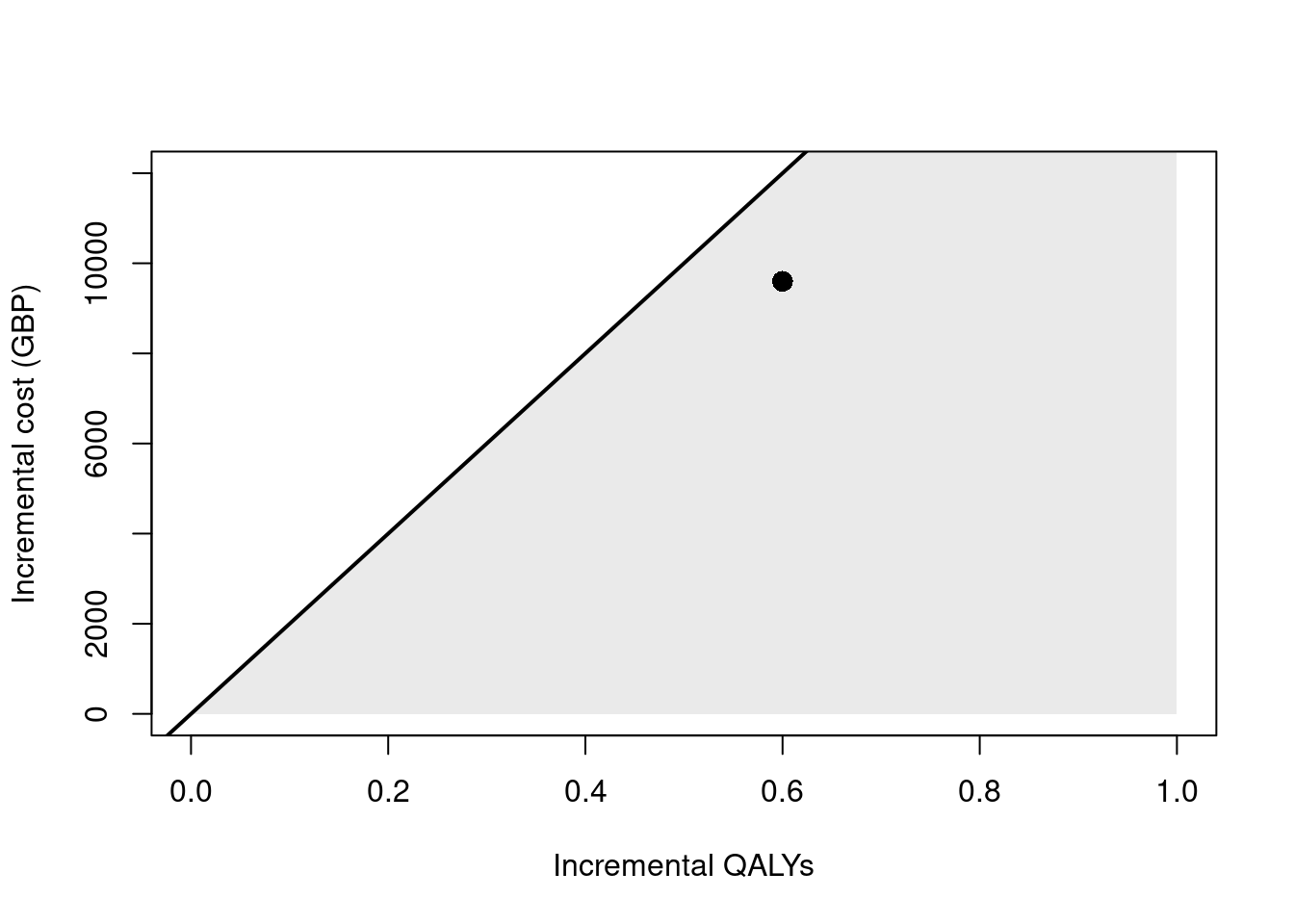
inmb <- q_incr*k - c_incrThe ICER is £16,000 per QALY. This is the incremental cost of Drug A relative to Drug B, scaled by the incremental effectiveness of Drug A relative to Drug B. The cost-effectiveness plane for this output is shown in Figure 8.5. The diagonal line represents the willingness to pay threshold of £20,000 per QALY and the “sustainability area” is shaded in grey. In this case, Drug A is cost-effective relative to Drug B. Finally, the INMB is £2,400.
Probabilistic Sensitivity Analysis (PSA)
Following from Section 8.6, to extend the model to perform a PSA we shall replace the point estimates for costs and QALYs used previously by \(S = 500\) random samples drawn from appropriate distributions. For this example, we will fix the probability point values associated with branches from chance nodes. We could think of this as if we knew the probabilities so accurately that \(p(\boldsymbol{p})\) is close to a one-point distribution at the true value). To include the node transition probabilities in the PSA the principle will be the same as for the other parameters. We will draw from Gamma distributions centred around the point estimates for the cost and health values \(r \sim \mbox{Gamma}(k, \mu)\) using the rgamma(shape, scale) function in R. When the costs are not close to zero and the distribution is more symmetrical we could justifiably alternatively use a Normal distribution with parameters on the natural scale. In our example the standard deviations are simply chosen as something convenient and sensible as approximately £1,000 for all costs and 3 QALYs for all QALYs. We use the properties that \(\mbox{E}(r) = k \mu\) and \(\mbox{Var}(r) = k \mu^2\) (see Section 4.3.4) to calculate the parameters corresponding to these assumptions. Of course, in a real analysis this should be determined using empirical information and expert knowledge. Applying this approach gives the Gamma distributions parameter values shown in Table 8.3.
| Type | Drug | Parameter | $k$ | $\mu$ |
|---|---|---|---|---|
| QALYs | A | $q_{succ}^A$ | 30/0.3 | 0.30 |
| QALYs | A | $q_{fail}^A$ | 25/0.6 | 0.60 |
| QALYs | B | $q_{succ}^B$ | 15/0.36 | 0.36 |
| QALYs | B | $q_{fail}^B$ | 23/0.39 | 0.39 |
| Cost | A | $c_{drug}^A$ | 2000/500 | 500.00 |
| Cost | A | $c_{succ}^A$ | 10000/100 | 100.00 |
| Cost | A | $c_{fail}^A$ | 20000/50 | 50.00 |
| Cost | B | $c_{drug}^B$ | 150/666 | 666.00 |
| Cost | B | $c_{succ}^B$ | 5000/200 | 200.00 |
| Cost | B | $c_{fail}^B$ | 10000/100 | 100.00 |
In this section, we will append the variable names with *_psa to emphasise the distinction with the previous point value analysis. Denoting the sample size \(S\) in R as n_samples, we can obtain the draws \(c^d_{drug, (s)},\; d = \mbox{A}, \mbox{B},\; s = 1, \ldots, S\) by specifying the n argument to the data generation function.
n_samples <- 500   # sample size

c_drug_psa <- rbind(
  `Drug A` = rgamma(n = n_samples, shape = c_drug["Drug A"]/500, scale = 500),
  `Drug B` = rgamma(n = n_samples, shape = c_drug["Drug B"]/666, scale = 666)
)
This results in a wide matrix with drug on the rows and sample on the columns. E.g. the first five columns of random samples are
round(c_drug_psa[ , 1:5], digits = 2) [,1] [,2] [,3] [,4] [,5]
Drug A 3275.02 2739.11 1232.46 1520.06 2096.12
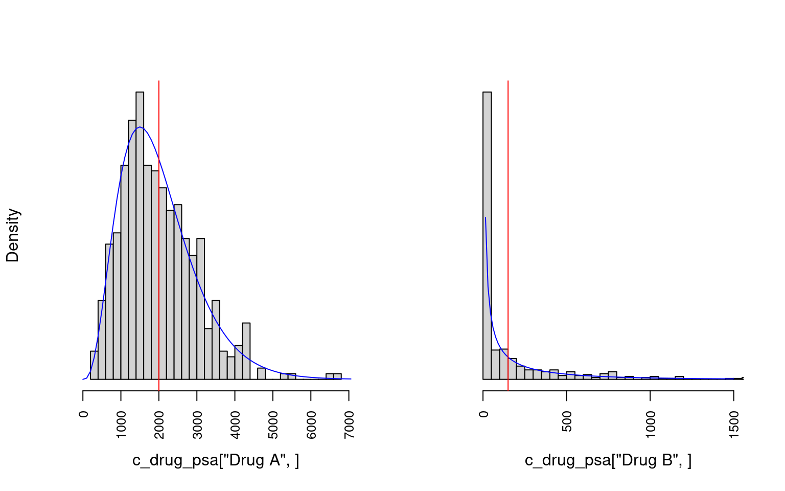
Drug B 3.83 0.16 336.78 0.38 19.49Figure 8.6 shows example histograms of the distributions of costs for the two drug treatments used in the PSA.
Next, we shall create the other cost and QALY samples in the same way to obtain the full set of PSA samples, \(\boldsymbol{\theta}^d_{(s)},\; d = \mbox{A, B}, \; s = 1, \ldots, S\).
c_success_psa <- rbind(
  `Drug A` = rgamma(n_samples, shape = c_success["Drug A"]/100, scale = 100),
  `Drug B` = rgamma(n_samples, shape = c_success["Drug B"]/50, scale = 50)
)

c_failure_psa <- rbind(
  `Drug A` = rgamma(n_samples, shape = c_failure["Drug A"]/200, scale = 200),
  `Drug B` = rgamma(n_samples, shape = c_failure["Drug B"]/100, scale = 100)
)

q_success_psa <- rbind(
  `Drug A` = rgamma(n_samples, shape = q_success["Drug A"]/0.3, scale = 0.3),
  `Drug B` = rgamma(n_samples, shape = q_success["Drug B"]/0.36, scale = 0.36)
)

q_failure_psa <- rbind(
  `Drug A` = rgamma(n_samples, shape = q_failure["Drug A"]/0.6, scale = 0.6),
  `Drug B` = rgamma(n_samples, shape = q_failure["Drug B"]/0.39, scale = 0.39)
)
Care must be taken to format the matrices so that the vector arithmetic is correct. That is, the dimension assignment and order of items is important. For example, c_total_psa is in row-major order where for each drug the realisations from the gamma distribution are along a row. If the vectorisation is done correctly then exactly the same code as for the point estimate case can be used.
c_total_psa <- c_drug_psa + (p_success*c_success_psa + p_failure*c_failure_psa)
q_total_psa <- p_success*q_success_psa + p_failure*q_failure_psa
Again, the incremental values can be obtained similarly to the point estimate case. However, now a whole row of values is used instead of a single value so we use the indexing syntax of a comma followed by a space
c_incr_psa <- c_total_psa["Drug A", ] - c_total_psa["Drug B", ]
q_incr_psa <- q_total_psa["Drug A", ] - q_total_psa["Drug B", ]
In comparison with the point value case presented previously, we now use the mean of each PSA sample to calculate the ICER and INMB.
icer_psa <- mean(c_incr_psa)/mean(q_incr_psa)
inmb_psa <- k*mean(q_incr_psa) - mean(c_incr_psa)
The ICER is £18,189 per QALY. This is similar to the ICER calculated with the point values. The expected INMB for £20,000 per QALY willingness to pay is £956 with 95% confidence interval (£-5785, £7697).
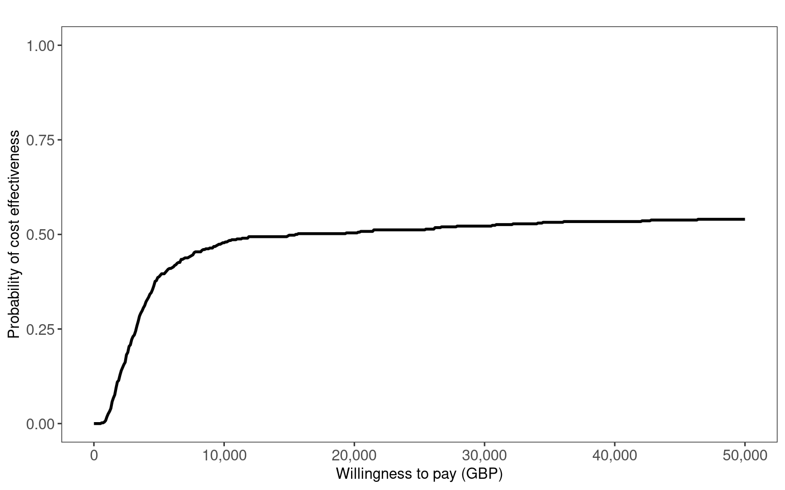
In Figure 8.7 (a) and Figure 8.7 (b), we use the contour2 and ceac.plot functions from the BCEA package to create the cost-effectiveness plane and cost-effectiveness acceptability curve, respectively. These clearly show the uncertainty about the optimal decision between Drug A or B. The ICER is close to the willingness to pay threshold and is relatively close to zero incremental QALYs. Thus, the CEAC plateaus at around 0.5.
library(BCEA)
bcea_psa <- bcea(t(q_total_psa), t(c_total_psa),
                 interventions = c("Drug A", "Drug B"), ref = 1)
contour2(bcea_psa, title = "", wtp = 20000, point = list(sise = 1),
         xlim = c(-10,10), ylim = c(-1000, 14000), graph = "ggplot2",
         xlab = "Incremental QALYs", ylab = "Incremental cost (GBP)")
ceac.plot(bcea_psa, ref = 1, title = "", graph = "ggplot2",
          xlab = "Willingness to pay (GBP)")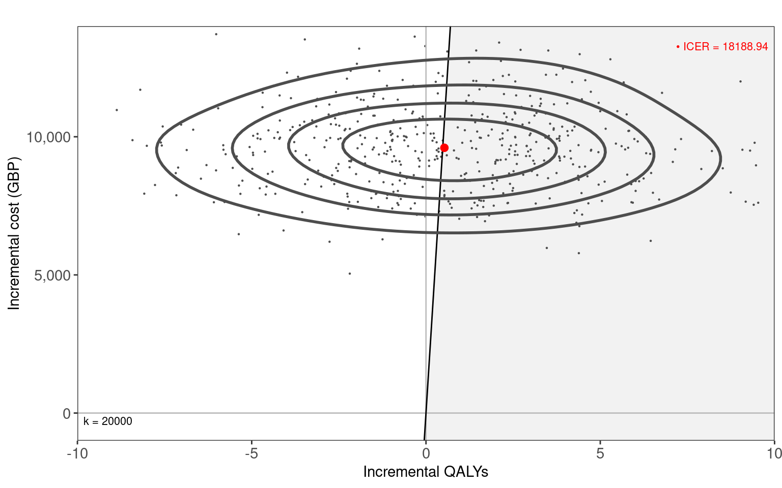
8.7.2 Folding back computation
Implementing the folding back method as described in Section 8.5.2.1 requires a different approach. For the forward method we explicitly scripted the model. Because folding back of a decision tree is a recursive, process we will use a recursive function i.e. one that calls itself. At first this may seem less clear than the forward approach but in fact taking a recursive paradigm can lead to simpler and easier to follow solutions. In this section, we will append the variable names with *_recur to clearly indicate that these are for the recursive formulation of the model. In order to use the recursive function we must first structure the input data so that we can traverse the tree.
The two common ways of doing this are with either an adjacency matrix or adjacency list. The choice of which to use depends on the structure of the tree and the specific problem. We shall adopt an adjacency list for our example. In R, a common way of doing this is to use a list object of parent and child nodes. The list names are the parent indices and the vector to the right-hand side are the child indices, which may be empty at the terminal nodes.
tree <-
  list("1" = c(2,3),  # root node
       "2" =  c(),    # terminal node
       "3" =  c())    # terminal node

tree
$`1`
[1] 2 3
$`2`
NULL
$`3`
NULLThe tree object represents the information that node 1 has children 2 and 3, nodes 2 and 3 have no children i.e. terminal nodes. This corresponds to one of the drug decisions in Figure 8.2.
Next we need to provide the probabilities, and cost and QALYs for this decision tree model in an appropriate format. Let us reuse the defined quantities *_success, *_failure from the previous forward analysis and create a list of dataframes of “node”, “probability” and “value” for each drug. Setting up the input data in this way means that we will be able to easily loop over the different drug scenarios with our recursive function.
data_cost_recur <- list(
  "Drug A" = data.frame(
    node = 1:3,
    prob = c(NA, p_success["Drug A"], p_failure["Drug A"]),
    # costs
    vals = c(c_drug["Drug A"], c_success["Drug A"], c_failure["Drug A"])
  ),
  "Drug B" = data.frame(
    node = 1:3,
    prob = c(NA, p_success["Drug B"], p_failure["Drug B"]),
    # costs
    vals = c(c_drug["Drug B"], c_success["Drug B"], c_failure["Drug B"])
  )
)

data_qaly_recur <- list(
  "Drug A" = data.frame(
    node = 1:3,
    prob = c(NA, p_success["Drug A"], p_failure["Drug A"]),
    # QALYS
    vals = c(0, q_success["Drug A"], q_failure["Drug A"])
  ),
  "Drug B" = data.frame(
    node = 1:3,
    prob = c(NA, p_success["Drug B"], p_failure["Drug B"]),
    # QALYS
    vals = c(0, q_success["Drug B"], q_failure["Drug B"])
  )
)
This format combines the data we used in Section 8.7.1 into a single object. The dataframes are in what is called “long” format (in contrast to “wide”). Notice that the root node 1 has probability NA. This is because since the root node has no preceding nodes it has no associated probability. The NA can also be used to identify when the root node has been reached in the recursive algorithm.
data_cost_recur$`Drug A`
node prob vals
1 1 NA 2000
2 2 0.7 10000
3 3 0.3 20000
$`Drug B`
node prob vals
1 1 NA 150
2 2 0.95 5000
3 3 0.05 10000A recursive folding back function for calculating the expected values at a node is given below. This version assumes a binary tree structure. The function ev_recursive takes the current node, the tree structure, and the data for the values and probabilities. The function checks if the current node is a terminal node and if so returns the value at that node. If not, the function calculates the expected value of the children nodes and returns the sum of the current node value and the weighted sum of the expected values of the children nodes. The function is called recursively for each child node.
ev_recursive <- function(node,   # current node
                         tree,   # list object
                         dat) {  # dataframe object

  # is this a terminal node?
  # if so then end early
  if (is.na(node)) {
    return(0)
  }

  # value at current node
  c_node <- dat$vals[dat$node == node]

  # tree structure starting from current node
  child <- tree[[node]]

  if (is.null(child)) {
    return(c_node)
  } else {

    # probabilities along each branch
    pL <- dat$prob[dat$node == child[1]]  # left branch
    pR <- dat$prob[dat$node == child[2]]  # right branch

    # check for NA values
    if (any(is.na(pL))) pL <- 0
    if (any(is.na(pR))) pR <- 0

    return(c_node +
             pL*ev_recursive(child[1], tree, dat) +
             pR*ev_recursive(child[2], tree, dat))
  }
}
This can be compared with Equation 8.1. A call to ev_recursive requires the tree list object for the decision tree structure, dat for the values and probabilities and node to tell it where to start the recursion. If we step through the calculation using our simplified example, consider the Drug A option then the first iteration gets the cost at the starting node £2000 (c_node) and gets the probabilities associated with the current node’s children, in this case probability of success 0.9 and failure 0.1. The current cost is then added to the weighted mean of the expected costs of the two children nodes. These expected costs are calculated in exactly the same way as we’ve just done, hence the recursive behaviour. For example, for the success branch this means getting the cost at the node of £10000 and then checking if there are any children, which there are not, so the function simply returns the current cost c_node. Once we reach the terminal states such as this then we can think of the expected costs being folded back recursively.
We are now ready to calculate the expected total costs and QALYs. We calculate ev_recursive separately for cost and QALYs, passing the data for the particular branch values, in this case data_cost_recur and data_cost_recur.
root <- names(tree)[1]  # index of root node

c_total_recur <- q_total_recur <- setNames(
  vector(mode = "numeric", length = 2L), c("Drug A", "Drug B")
)

for (i in 1:2) {
  c_total_recur[i] <- ev_recursive(node = root, tree, data_cost_recur[[i]])
  q_total_recur[i] <- ev_recursive(node = root, tree, data_qaly_recur[[i]])
}
Equivalently, we can calculate the cost and QALYs for both drugs in a single step by mapping through the list of inputs. This is a more compact way of looping over inputs. The base R version of the function to do this is the lapply function from the apply family of functions. Here, we use the map_dbl equivalent from the purrr package (part of the tidyverse) simply because it returns an atomic vector rather than a list. The tilde ~ and dot . are used in the map functions as a shorthand in place of writing the equivalent but longer anonymous function function(x) ev_recursive(node = root, tree, x). The base R equivalent is to instead use \(x) and x, respectively.
c_total_recur <- purrr::map_dbl(
  data_cost_recur, ~ev_recursive(node = root, tree, .)
)
q_total_recur <- purrr::map_dbl(
  data_qaly_recur, ~ev_recursive(node = root, tree, .)
)
Now, in the same way as we did for the forward approach, we can calculate the incremental costs and QALYs.
c_incr_recur <- c_total_recur["Drug A"] - c_total_recur["Drug B"]
q_incr_recur <- q_total_recur["Drug A"] - q_total_recur["Drug B"]
The ICER can now be calculated as the ratio of incremental costs to incremental QALYs.
icer_recur <- c_incr_recur/q_incr_recurThe ICER is £16,000 per QALY, the same as for the forward approach.
For our running example, this folding back approach is arguably a bit too elaborate relative to simply writing out the decision tree equations explicitly. There is always a balance between readability, reusability, and concise code. Different data formats and algorithms may be better suited for different problems depending on the structure of the tree. Computational cost is less of a concern for our example but for more complicated trees it may be a valid issue and should also be considered.
NoteExtra code
The specific code used to calculate the parameters \(p^*\), \(c^*\) and \(q^*\) can be found in the online version of this book, which is available at the website https://gianluca.statistica.it/books/rhta)
8.8 When decision trees should not be used
Decision trees are not appropriate where diseases exhibit long latencies after a clinical intervention, or where conditions require multiple interventions over extended time periods. Where these circumstances apply, it is not realistic to assign an instantaneous cost and outcome after each chance node, since these variables may not observed for a considerable period of time. Many unmodelled variables may affect the ultimate value of costs and outcomes experienced by patients over a long span of time, including not only other diseases experienced by patients but also the emergence of new interventions with distinct cost-effectiveness profiles.
The influence of time and time dependency is not easily represented in decision trees. Patient progress through the decision tree to reach a terminal node is unidirectional. Travel “back and forth” over the branches of a decision tree is not permitted. In Figure 8.1, we see how pathways necessarily traverse from the root node on the lefthand side to the terminal nodes on the righthand side. This means that, for example, disease recurrence is not readily accounted for. In many clinical contexts, the possibility of recurrence is critical, particularly where pathologies are treatment refractory or the underlying biological processes of a disease (such as cancer) naturally gives rise to consideration of recurrence.
In principle, multiple branches corresponding to different time intervals, recurrence and other time-dependent structures could be modelled. However, analysis of “bushy” trees rapidly becomes complex and inefficient given their intensive data requirements and the challenges of analysing and interpreting many different pathways.
In practice, alternative decision analytic models, such as Markov models (Siebert et al., 2012) and discrete event simulations (Karnon et al., 2012) and other related modelling approaches may be better suited to those circumstances where longer time intervals and time-dependence are important to the decision-making context at hand. Some of these models are considered in Chapter 9, Chapter 11 and Chapter 12. However, a decision tree may still be useful when combined with more involved models. For example, terminal nodes on a tree could be replaced with further branches to time-dependent processes. This is a common approach in health technology assessment, where decision trees are used to model diagnostic tests and screening programmes, and are then combined with long-term population models.
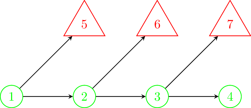
By way of an example, Figure 8.8 (a) shows an example of a decision tree type model where the same structure is duplicated several times. That is, from state 1 it is possible to transition to either another chance node or a terminal state. If traversed to the chance node then once again the same possible transitions are available and so on. We will assume that all of the chance nodes are identical. This same structure could be repeated for many cycles and lead to an unwieldy tree. Common examples like this occur when there is possible mortality at each time step e.g. death from cancer each year. Clearly, this is a cumbersome and inefficient way to represent this process.
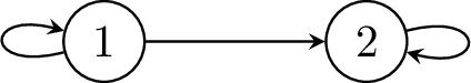
Figure 8.8 (b) offers an alternative way to represent this same process in a much simpler and compact way; allowing transitions back to a previous state or for no transition i.e. a transition to itself. In comparison, state 1 is equivalent to all of the chance nodes in Figure 8.8 (a) and state 2 is a sink state equivalent to all of the terminal states in Figure 8.8 (a) since the only possible transition is to itself. The arrow from state 1 to state 2 in Figure 8.8 (b) is equivalent to all of the arrows from the chance nodes to the terminal nodes in Figure 8.8 (a), and the arrow from state 1 back to itself in Figure 8.8 (b) is equivalent to all of the horizontal arrows between change nodes in Figure 8.8 (a). The model represented by Figure 8.8 (b) also has no limit on how many cycles are permitted before reaching a terminal state.
8.9 How are decision trees used in HTA?
We have seen that decision trees are best suited to contexts where there is little or no time dependence, in which scale of the model is tractable for analysis, and for which appropriate data may be obtained.
Decision trees are uniquely well suited for modelling diagnostic technologies and screening programmes. False positives, true positives, false negatives, and true negatives could each be nodes flowing from the parent node, representing a diagnostic or screening intervention, in the tree. The consequences of these outcomes could be a single value for costs and QALYs, or could lead into a long-term disease model such as Markov model. For these reasons, an important use of decision trees in HTA is the evaluation of diagnostic tests, albeit often in conjunction with more complex decision analytic models. Diagnostic tests may be used to stratify patients to particular treatments and forms of clinical management.
For example, Yang et al. (2019) reviewed UK National Institute for Health Research (NIHR) Health Technology Assessment reports which were published between 2009 and 2018 in order to evaluate the methods used to model the cost-effectiveness of diagnostic tests using decision analytic modelling. Of the 55 studies which met the inclusion criteria, decision trees were the most common model structure in 38 or 69% of studies, either alone (\(n=23\), \(42\)%) or combined with a more complex model incorporating time-dependent structures (\(n=15\), \(27\)%). Two recent examples of this combination of decision trees with more complicated time-dependent modelling are Elwenspoek et al. (2022) and Welton et al. (2017). Elwenspoek et al. (2022) developed decision-analytic models to identify adults and children with coeliac disease, a chronic autoimmune disorder, and to determine the cost-effectiveness of active case-finding strategies in primary care. The model was a combination of a decision tree followed by a Markov model. The decision tree was used to characterise different testing strategies that could be used to identify coeliac disease. The Markov model reflected the costs and health consequences associated with diagnosed or undiagnosed coeliac disease, and therefore measured the benefits of initial detection of this disease using the processes represented in the disease tree. A similar approach was followed by Welton et al. (2017), who evaluated the accuracy of screening tests for atrial fibrillation, a disorder characterised by irregular heart rhythms. A decision tree was used to characterise diagnostic test accuracy, and a Markov model that accounted for longer-term disease processes and impacts on costs and QALYs was used to assess the cost-effectiveness of different screening strategies for atrial fibrillation.
8.10 Conclusion
This chapter introduced the use of decision trees as a first type of decision-analytic model. Decision trees offer a relatively straightforward means of making transparent the choices, uncertainties, costs and outcomes associated with different treatment modalities. They are inherently comparative, since the optimal choice in a decision tree involves optimising over the expected value of different courses of action. For this reason, they are a useful first tool in health technology assessment. They are also readily structured to reflect sequences of clinical decision-making.
The use of decision trees is best limited to contexts where time dependency and long-term disease processes or outcomes are not relevant (see e.g. Yang et al., 2019). Other forms of decision-analytic models will be more appropriate in those contexts, although decision trees are still useful as adjuncts to more complicated models. This may be as a quick, rough representation useful for development and checking, or to form part of the overall model.
There are a number of advantages to using R for creating decision trees, especially in comparison to the use of MS Excel. In particular, when there are more than a small number of decision and chance nodes, the number of terminal nodes increases. In these cases, the vectorisation and matrix multiplication capabilities (amongst others) of R render substantial efficiency advantages to analyst. Very rapid backward computation of decision trees, even if complex, is readily facilitated by R’s capacity to handle iteration and recursion (see Chapter 2).