n_treatments <- 3
treatment_names <- c("Observation", "Lev", "Lev+5FU")9 Cohort Markov Models in Discrete Time
Howard Z Thom
University of Bristol, UK
Pedro Saramago
University of York, UK
Marta Soares
University of York, UK
Eline Krijkamp
Erasmus University Rotterdam, Netherlands
Felicity Lamrock
Queen’s University Belfast, UK
9.1 Introduction
In Chapter 8, we saw the decision tree, which is one of the simplest approaches to modelling for cost-effectiveness analysis. Decision trees are appropriate if the time horizon of the decision problem is short and if there are few repeat events. If the time horizon of the decision problem is longer and if events repeat, representations with decision trees can become overly complex, with many branches and a bushy appearance. In this chapter, we will explain the theory and implementation of cohort Markov models, which are useful for decisions with long-term consequences and potentially repeating events (Briggs et al., 2006; Siebert et al., 2012). Examples include modelling of chronic diseases such as psoriatic arthritis or multiple sclerosis, in which severity or disability can progress over time (Baharnoori et al., 2022; Thom et al., 2015). They are also useful for diseases characterised by periods of relapse and remission, as found in mental health conditions such as bipolar disorder (Kleijburg et al., 2022). Markov models are a special case of multistate models, which will be further explored in Chapter 11, and which are themselves an extension of survival modelling to more than two states (Beyersmann et al., 2012; Kalbfleisch and Prentice, 2002).
In line with other modelling approaches to cost-effectiveness analysis, Markov models can be used to synthesise evidence from various data sources, including clinical trial findings, cross-sectional studies on utilities, or listed drug prices, to create a comprehensive overview of the effect of an intervention (Alarid-Escudero et al., 2023a). Markov models can furthermore extrapolate this combined data into the future, which offers valuable insights into the long-term effects of an intervention, which are essential for healthcare decision making (Alarid-Escudero et al., 2023a; Green et al., 2023) .
To simulate the nature of disease progression, and to estimate the expected health outcomes and costs, Markov models must first characterise a disease into health states (Briggs et al., 2006; Siebert et al., 2012). These states must be collectively exhaustive and mutually exclusive, which means that individuals must be in one health state at any moment in time but cannot be in more than one health state (Green et al., 2023; Jackson, 2011). The chosen health states must represent the important clinical and economic aspects of the disease, in order to offer a comprehensive overview of the impact of a healthcare strategy on an individual’s lifetime. The Dead state, if relevant to the study, can also be subdivided into all-cause and cause-specific mortality. This distinction allows for a more detailed understanding of the reasons behind individual mortality.
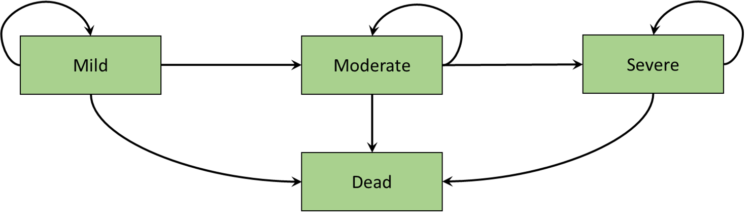
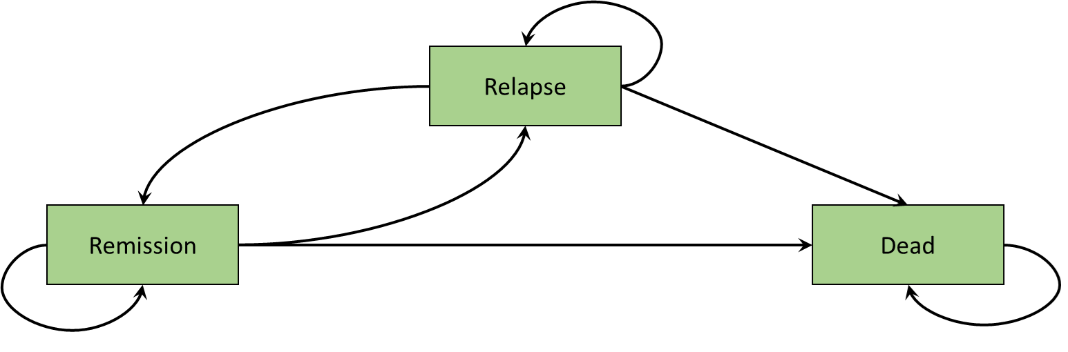
An example of a Markov model representing disease progression is illustrated in Figure 9.1 (a). This state-transition diagram shows the health states defined as squares and the arrows represent permitted movements of individuals between health states. These movements between health states are called transitions. In this hypothetical disease progression model, patients can only progress to more severe states. Such a model is termed irreversible. An example of a Markov model representing remission and relapse is illustrated in Figure 9.1 (b). Unlike the disease progression model of Figure 9.1 (a), individuals can transition in either direction between remission and relapse. In both the disease progression and remission relapse models, the Dead state is included as a single state to which individuals can transition from any state. Furthermore, there are no transitions back from the Dead state, and such states are named absorbing (Green et al., 2023).
We will elaborate on these concepts, and provide an implementation in R, using a fully worked cost-effectiveness model in colon cancer.
9.2 Colon Cancer Example
Our case study for this chapter is the historical comparison of the cost-effectiveness of two new post-surgical adjuvant therapies for colon cancer with no treatment. The three treatment options are
- Observation (Obs), i.e. no treatment
- Levamisole (Lev)
- Levamisole and fluorouracil (Lev+5FU)
To answer this research question, we will develop a cohort Markov model and implement it in R. The different components of a Markov model will be described in a step-by-step process, with important concepts explained as they are encountered. The data for the model is derived from the colon dataset from the survival package. This dataset represents a randomised clinical study that was performed in the 1980s to investigate the efficacy of post-surgery adjuvant therapy for colon cancer (Moertel et al., 1995; Moertel et al., 1990).
The first part of the R code is provided in Box 9.1 and defines the treatment options as global variables.
9.2.1 R Packages for Markov modelling
The packages used in this chapter are listed in Box 9.2. Recall that packages not already installed on your machine need to be installed using the R command install.packages("X"). Functions from each of these packages are explained as they occur.
library(heemod)   # For illustrating state-transition diagram of Markov models
library(BCEA)     # For analyzing the costs and effects of the model
library(MASS)     # For multivariate normal
library(survival) # For colon cancer dataset
library(flexsurv) # For Gompertz survival functions
library(diagram) # For visualizing graphsThere are two useful R packages for cohort Markov modelling R, namely heemod and hesim. However, in this chapter, we will implement all model logic in base R as it will solidify understanding of Markov models but also provide flexibility to implement functionality not envisaged by the heemod or hesim packages. The hesim package will described in detail in Chapter 11 and is not used further in the present chapter.
9.2.2 Describing and Displaying Health States in the colon Markov model
The following health states are used to describe the important health outcomes and costs in colon cancer:
- Recurrence-free
- Recurrence
- Dead (All-cause)
- Dead (Cancer)
We implement this information in R in the following code.
# number of health states
n_states <- 4
# names of the health states
state_names <- c(
  "Recurrence-free", "Recurrence", "Dead (All-cause)", "Dead (Cancer)"
)
These health states and allowed transitions are illustrated in Figure 9.2 (a). Individuals begin in the Recurrence-free health state and can move to recurrence or either of the dead states. Individuals who are in the recurrence health state can not return to the recurrence free health state. They can only move to one of the dead states. The model is therefore irreversible and thus similar to the disease progression model in Figure 9.1 (a). Individuals can remain in either Recurrence-free and recurrence over time. The dead states are again absorbing.
The value of the transition probabilities need to be calculated and organised into a so-called transition matrix, where the rows represent the health state the individual is currently in and the columns the health states to which the individual can transition. The heemod package has the useful feature that it can display health states and possible transitions if provided with a transition matrix. Box 9.3 displays the code to create the state transition matrix of the colon cancer model.
health_states_diagram <-
  define_transition(
    state_names = c(
      "Recurrence-free", "Recurrence", "Dead (All-cause)", "Dead (Cancer)"
    ),
    X1, X2, X3, 0,
    0,  X4, X5, X6,
    0,  0,  X7, 0,
    0,  0,  0,  X8
)heemod package
The graphical representation of the underling transition matrix can be visualised using the heemod plotting facilities, as in the following R code.
# Note: the arguments box.size, relsize and self.cex are case specific.
# The basic code to plot would be: plot(health_states_diagram)
plot(health_states_diagram, box.size = 0.18, relsize = 0.75, self.cex = 0.5)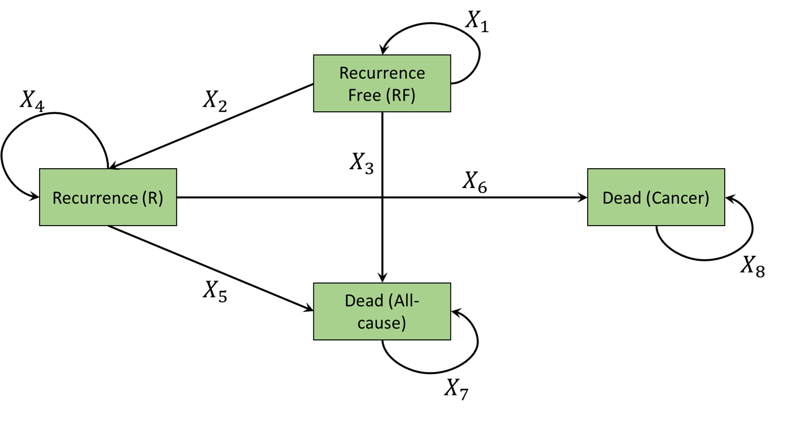
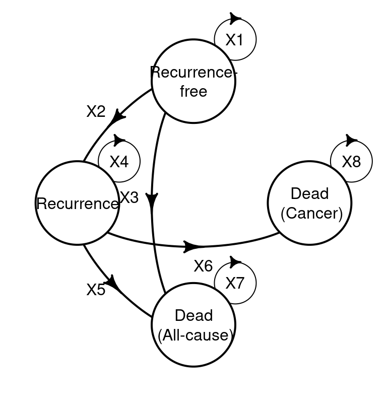
heemod representation of the graph associated with the transition matrix
Comparing Figure 9.2 (b) with Figure 9.2 (a) provides a simple check that the model has been correctly specified. The four by four structure positioning of values of X are such that if a transition is possible an X is placed in that position. For example as it is possible to move from Recurrence-free to Recurrence, X2 denotes this movement. As transitions are not possible from dead states, a 0 is placed in those positions.
9.3 General features of cohort Markov models
9.3.1 Continuous and discrete time
In a continuous-time model, transitions of individuals between health states can happen at any time along a continuous interval (Beyersmann et al., 2012; Soares and Castro, 2012; Williams et al., 2017). In a discrete-time model, transitions occur only at discrete time points, e.g. daily or annual. In state-transition models, these discrete times periods are called cycles (Naimark et al., 2008). The duration of these cycles is determined by the nature of the disease and the interventions under evaluation, and can be any time scale but are often monthly or yearly. The chosen duration must be sufficiently short to capture relevant events. In reality, individuals can transition between health states in continuous time, so using a discrete-time approximation may introduce bias in the results. This bias is associated with the chosen cycle length and the nature of the disease, as well as the model structure and model parameters (Alarid-Escudero et al., 2023a; van Rosmalen et al., 2013). The bias from using discrete time can be reduced by using shorter cycle times, but this must be balanced against the need for granular data to accurately estimate probabilities for such shorter cycles. Within-cycle correction, e.g. half-cycle correction, had also been suggested and often used to correct for the bias from using discrete time (Naimark et al., 2008; Srivastava et al., 2020). Chapter 11 will discuss the use of continuous-time modelling, while the present chapter discusses discrete time modelling.
After each Markov model cycle, an individual has a probability of transitioning to certain health states. In Box 9.3, the transition probabilities between health states in the example are the values of X. In this example, an annual cycle length has been chosen. The number of cycles is equal to the time horizon of the Markov model. If a disease has lifetime impacts, a lifetime horizon should be chosen (NICE, 2022). To reflect a lifetime horizon of the individuals in the colon cancer model, the total number of cycles is set to 50 cycles, as shown in Box 9.4.
n_cycles <- 509.3.2 Hazard rates, ratios, probabilities, odds, and odds ratios
Transitions between health states in a discrete-time cohort Markov model are governed by probabilities, while those in a continuous time model are governed by rates (Alarid-Escudero et al., 2023a; Jackson, 2011). Rates, or hazard rates, are an instantaneous measure that ranges from zero to infinity. Rates describe the number of transitions between health states for a given number of individuals per unit of time. In contrast, probabilities describe the likelihood that an individual will transition between health states in a given time period, which is the cycle length, and range from 0 to 1. These probabilities are conditional on the currently occupied state (Beyersmann et al., 2012).
It is possible to use published or otherwise available transition probabilities for your models. However, a transition probability may not exist for the cycle length of your model. In such a case it would be necessary to transform transition probabilities from one time frame to another. Suppose a 5-month probability of a heart attack is reported in the literature but that your model uses a 1-month cycle length and thus needs a 1-month probability. If the rate is constant over time, a 5-month rate could be converted to a 1-month rate through division by 5, but this is not true for probabilities. Under an assumption of constant rate of event, and two events only, we can convert from a rate \(r\) to probability \(p\) over time \(t\) using \[ p(t) = 1 - e^{-rt} \] To change the time frame of a probability the probability needs to be converted to a rate using this formula, scaled to the new time frame, and then converted back to a probability. This return conversion from a probability \(p\) over time \(t\) to a rate \(r\) is performed using \[ r(t)= -\frac{\log{(1-p)}}{t} \]
The code in Box 9.5 uses this approach to scale a 5-month probability of 50% to a 1-month probability of 12.9%.
r <- -log(1 - 0.5)/5
prob_1_month<- 1 - exp(-r * 1)Another commonly reported summary statistic for events associated with transitions are odds or odds ratios. The odds of an event are the ratio of the probability of the event occurring \(p\) the probability of it not occurring \((1-p)\). \[
\mbox{odds} = \frac{p}{1-p}
\] The odds ratio for some treatment \(1\) with event probability \(p_{1}\) compared to treatment \(2\) with probability \(p_{2}\) is the ratio of the odds \[
\mbox{OR} = \frac{p_{1}}{1-p_{1}} / \frac{p_{2}}{1-p_{2}}
\] Log odds can be converted to the probability scale using the inverse of the logistic function, and the resulting probability is over the same time as that used to measure the log odds. A probability can be translated to the log odds scale using the logistic function. This may be necessary if treatment effects are given as (log) odds ratios; the log odds of a reference treatment can be added to the log odds ratio for a comparator, and the result can be translated to a probability. Box 9.6 gives two functions, one to convert from log odds to probabilities using the inverse logistic function, which we name expit, and another to convert from probabilities to log odds, which we name logit.
# Function to translate log odds to probabilities
expit <- function(logO) {
  return(exp(logO)/(1 + exp(logO)))
}

# Function to translate probabilities to log odds
logit <- function(p) {
  return(log(p/(1-p)))
}expit(0.5)[1] 0.6224593logit(0.6224593)[1] 0.49999999.3.3 Markov and semi-Markov models
Markov models are characterised by a memoryless property called the Markov assumption or Markov property. Under the Markov assumption, movement of an individual from their current health state to a future one, conditional on both past and current health states, depends only on the current health state of the individual and not the past health states (Jackson, 2011; Kalbfleisch and Prentice, 2002). A semi-Markov model relaxes this assumption so that transition rates can also depend on the sojourn time, which is the time spent in the current state. In this sense, a semi-Markov model is a clock-reset model (Green et al., 2023; Meira-Machado et al., 2009). Time in a Markov model is defined as time since initiation of the model, so is termed clock-forward. Markov and semi-Markov models are both examples of multistate models, which are further discussed in Chapter 11, but in this chapter we consider only Markov models.
9.3.4 Cohort and individual level models
Multistate models can be executed at either the cohort or individual level (Davis et al., 2014; Siebert et al., 2012). Cohort models simulate a closed group of individuals who are assumed to represent the “average” member of the target population (Ethgen and Standaert, 2012). Heterogeneity within the target population is not explicitly modelled. Individual level models also simulate a closed group but can be a heterogeneous sample from the target population. Cohort models are less computationally demanding as the individuals being the same means most calculations only need to be conducted once at the cohort level (Krijkamp et al., 2018). Individual levels are valuable for capturing heterogeneity, but this must be weighed against the need to simulate individual transition and estimate costs, and utilities for each individual makes them computationally intensive (Davis et al., 2014; Krijkamp et al., 2018). In this chapter, we consider only cohort level models and leave individual multistate models again for Chapter 11.
9.4 Time-homogeneous Markov model
9.4.1 Transition probabilities
In defining transition probabilities between health states it is necessary to decide if the probabilities will change over time. Time-homogeneous means that the transition probabilities between health states will be the same at each cycle of the model (Alarid-Escudero et al., 2023b; Jackson, 2011). Time-inhomogeneous means that transition probabilities between health states can change with time. A recognised example of a time-inhomogeneous transition probability is the probability of death increasing with age.
In Box 9.7 we first use an array function to assign memory for the transitions between health states for each treatment (Krijkamp et al., 2020). In this example we have a 4 by 4 matrix for each of the treatments. Transition probabilities for recurrence and cancer-related death were derived from the colon cancer dataset. They are calculated as the mean, over the 50 year time horizon, of the time-inhomogeneous probabilities that will be described in Section 9.5.1.
The transition probability matrix is a 4 by 4 matrix where rows sum to 1. The top left entry is the transition probability from Recurrence-free to Recurrence-free, the top right is the transition probability from Recurrence-free to Dead (Cancer). Probabilities from the Dead health states, or other absorbing states, to themselves are always 1 as individuals remain in those states indefinitely. If the matrix does not change over time it describes a time-homogeneous model. As an individual cannot return from recurrence to Recurrence-free, the first column of the second row would always be 0.
Background mortality follows a Gompertz distribution fitted to US lifetables, with further details given when discussing time-inhomogeneous survival models in Section 9.5.1. It is the same regardless of treatment and recurrence. As our model is time-homogeneous, we again assume it is the mean over the time horizon of 50 years (i.e., probability of 0.13).
The probabilities of remaining in the Recurrence-free and Recurrence states are 1 minus the probabilities of exiting the states, ensuring they sum to 1. This is implemented using a for loop as it is the same code for each state.
transition_matrices_homogeneous <- array(
  dim = c(n_treatments, n_states, n_states),
  dimnames = list(treatment_names, state_names, state_names)
)

# For the Observation option
transition_matrices_homogeneous["Observation", "Recurrence-free", ]  <-
  c(NA, 0.064, 0.13, 0)
transition_matrices_homogeneous["Observation", "Recurrence", ]       <-
  c(0, NA, 0.13, 0.44)
transition_matrices_homogeneous["Observation", "Dead (All-cause)", ] <-
  c(0, 0, NA, 0)
transition_matrices_homogeneous["Observation", "Dead (Cancer)", ]    <-
  c(0, 0, 0, NA)

# For the Lev treatment option
transition_matrices_homogeneous["Lev", "Recurrence-free", ]  <-
  c(NA, 0.067, 0.13, 0)
transition_matrices_homogeneous["Lev", "Recurrence", ]       <-
  c(0, NA, 0.13, 0.40)
transition_matrices_homogeneous["Lev", "Dead (All-cause)", ] <-
  c(0, 0, NA, 0)
transition_matrices_homogeneous["Lev", "Dead (Cancer)", ]    <-
  c(0, 0, 0, NA)

# For the Lev+5FU treatment option
transition_matrices_homogeneous["Lev+5FU", "Recurrence-free", ] <-
  c(NA, 0.046, 0.13, 0)
transition_matrices_homogeneous["Lev+5FU", "Recurrence", ]      <-
  c(0, NA, 0.13, 0.26)
transition_matrices_homogeneous["Lev+5FU", "Dead (All-cause)", ] <-
  c(0, 0, NA, 0)
transition_matrices_homogeneous["Lev+5FU", "Dead (Cancer)", ]    <-
  c(0, 0, 0, NA)

# Ensure the rows sum to 1
# Probability of remaining in current state is 1 minus probability of leaving
for(i_state in 1:length(state_names)) {
  transition_matrices_homogeneous[, i_state, i_state] <- 1 -
    rowSums(transition_matrices_homogeneous[, i_state, -i_state])
}We can visualise the full transition matrix and check that each of the rows sums to 1 using the following R code.
transition_matrices_homogeneous["Observation", , ] Recurrence-free Recurrence Dead (All-cause) Dead (Cancer)
Recurrence-free 0.806 0.064 0.13 0.00
Recurrence 0.000 0.430 0.13 0.44
Dead (All-cause) 0.000 0.000 1.00 0.00
Dead (Cancer) 0.000 0.000 0.00 1.00head(apply(transition_matrices_homogeneous, c(1), rowSums)) Observation Lev Lev+5FU
Recurrence-free 1 1 1
Recurrence 1 1 1
Dead (All-cause) 1 1 1
Dead (Cancer) 1 1 19.4.2 Markov trace and simulating disease progression
A key structure for Markov models, is the Markov trace. The Markov trace provides an overview of how the cohort is distributed over each health state in each cycle, in proportions. In our case example, everyone starts in the Recurrence-free health states. The Markov trace will show a 1 in the Recurrence-free health states, mean that 100% of the cohort starts in the Recurrence-free, while it will show a zero in all other health states (Box 9.8). Over time, individuals will transition to the other health states and the proportion will shift, with at the end of the simulation, the majority of the individuals will be in the dead health states.
The Markov trace is generated by using the transition probabilities to calculate movements between health states at each cycle of the model over the time horizon. Mathematically, given initial proportions for the cohort vector \(\pi_{0}\), proportions \(\pi_{t+1}\) at cycle \(t+1\) are calculated using the transition probability matrix \(\boldsymbol{P}\) and cohort vector \(\pi_{t}\) via matrix multiplication. By using matrix multiplication, we calculate which proportion of the individuals will make a transition form their current health state to the other health states and also sum this to get the overall proportion of each health states at the end of the cycle. The result of this multiplication gives us the distribution of individuals transitioning from their present health states to other states. For cohort simulations, matrix multiplication (see Note 4.1 in Section 4.6.2.2 and Section 2.4.3.3 for more details) is an efficient method, as it efficiently handles multiple steps of multiplication and addition simultaneously and therefore provides an efficient approach to simulate state distributions over time.
\[ \pi_{t+1} = \pi_{t}\boldsymbol{P} \]
# Proportion of cohort in each state during first cycle
cohort_vector_first <- c(1, 0, 0, 0)
cohort_vector_second <- cohort_vector_first %*%
  transition_matrices_homogeneous["Observation", , ]
cohort_vector_third <- cohort_vector_second %*%
transition_matrices_homogeneous["Observation", , ] Looking at the Markov trace is a simple way to check if the model is working correctly and, by considering the clinical situation being simulated, testing face validity. For example, if everyone begins in the recurrence free state at time 0, then we can use the transition probability for the Observation treatment in the first instance to calculate where the cohort will move. Box 9.8 illustrates the calculation of the Markov trace for the first, second and third cycle.
The calculated transition matrix and the resulting Markov traces can be visualised using simply calling the R objects that define them.
cohort_vector_second Recurrence-free Recurrence Dead (All-cause) Dead (Cancer)
[1,] 0.806 0.064 0.13 0cohort_vector_third Recurrence-free Recurrence Dead (All-cause) Dead (Cancer)
[1,] 0.649636 0.079104 0.2431 0.02816Of course we could repeat the above code for each cycle and for each treatment but it is easier to assign memory for the Markov trace and write generic code with a for loop. The code in Box 9.9 loops over cycles and treatments to generate the full Markov trace. The first dimension of the array is used to indicate the treatment, the second and third indicate the number of cycles and health states, respectively. For each intervention, all individuals start in the Recurrence-free health states, Markov_trace_homogeneous[, 1, 1] <- 1. The distribution of the cohort over the different health states over time is calculated by multiplying the Markov trace with the transition probabilities, using a loop. Box 9.9 shows the first cycles of the observation arm. It should be noticed that the sum of the rows of the Markov trace should always be one. This means the entire cohort is distributed among the health states, and that throughout the simulation no new individual entered or were lost.
Markov_trace_homogeneous <- array(
  0, dim = c(n_treatments, n_cycles, n_states),
  dimnames = list(treatment_names, paste("Cycle", 0:(n_cycles-1), sep = " "),
                  state_names)
)

# All individuals start in Recurrence-free
Markov_trace_homogeneous[, 1, "Recurrence-free"] <- 1

# Use transition matrix to update Markov trace at each cycle
for (i_cycle in 1:(n_cycles - 1)){
  for(i_treatment in 1:n_treatments) {
    Markov_trace_homogeneous[i_treatment, i_cycle + 1, ] <-
      Markov_trace_homogeneous[i_treatment, i_cycle, ] %*%
      transition_matrices_homogeneous[i_treatment, , ]
  }
}The following R code shows the first few rows of the Markov trace, for each observation arm and confirms that all rows sum to 1, as required.
# Present the first six cycles of the Markov trace for the observation arm
head(Markov_trace_homogeneous["Observation", , ])
Recurrence-free Recurrence Dead (All-cause) Dead (Cancer)
Cycle 0 1.0000000 0.00000000 0.0000000 0.00000000
Cycle 1 0.8060000 0.06400000 0.1300000 0.00000000
Cycle 2 0.6496360 0.07910400 0.2431000 0.02816000
Cycle 3 0.5236066 0.07559142 0.3378362 0.06296576
Cycle 4 0.4220269 0.06601514 0.4157319 0.09622599
Cycle 5 0.3401537 0.05539623 0.4791774 0.12527265# The rows of each cycle sum to 1, which means that all individuals occupy a
# health state
head(apply(Markov_trace_homogeneous, c(1), rowSums)) Observation Lev Lev+5FU
Cycle 0 1 1 1
Cycle 1 1 1 1
Cycle 2 1 1 1
Cycle 3 1 1 1
Cycle 4 1 1 1
Cycle 5 1 1 19.4.3 State Costs
The state costs depend on the treatment as the cost of spending one cycle in the Recurrence-free state depends on the probability of experiencing recurrence, which itself is treatment dependent. The cost of Recurrence-free is the cost of one-off advanced treatment by probability of experiencing recurrence, which we assume to be $40,000.
In cohort Markov models, costs are associated with states rather than the transitions, which represent events. It is therefore challenging to implement the cost of recurrence. The state cost of recurrence is the ongoing cost of having had a recurrence, rather than the one-off cost of the recurrence event itself. We therefore associate the cost of recurrence with the Recurrence-free state, but weight it by the probability of recurrence. On average, this adds the cost of recurrence events. This solution is implemented in Box 9.10, where cost of recurrence is multiplied by the probability of recurrence from the transition matrix. As the one-off cost of recurrence is counted in the Recurrence-free state, the recurrence state itself has zero cost per cycle. Costs of spending one cycle in each of the dead states is set to zero. It is straightforward to change all these costs if adapting this code to other applications.
state_costs <- array(0, dim = c(n_treatments, n_states),
                   dimnames = list(treatment_names, state_names))

state_costs[ , "Recurrence-free"] <-
  transition_matrices_homogeneous[, "Recurrence-free", "Recurrence"] * 40000
state_costs[, "Recurrence"]       <- 0
state_costs[, "Dead (Cancer)"]    <- 0
state_costs[, "Dead (All-cause)"] <- 0Again, simply calling the R object lets us visualise the output.
state_costs Recurrence-free Recurrence Dead (All-cause) Dead (Cancer)
Observation 2560 0 0 0
Lev 2680 0 0 0
Lev+5FU 1840 0 0 09.4.4 State QALYs
Utilities are assigned to each state of the Markov model. Multiplying each of these by the cycle length gives the Quality Adjusted Life Years (QALYs) accrued from spending one cycle in each state. In our example, the cycle length is one year, so QALYs per cycle are the same as the state utilities. The state QALYs are a defined in Box 9.11 as an array but are actually a simple 4-element vector as they do not depend on treatment or cycle. In our Markov model, the utility for Recurrence-free is 0.8, utility for recurrence is 0.6, and utility in the dead states is 0.
state_qalys <- array(dim = c(n_states), dimnames = list(state_names))

# QALY associated with 1-year in each health state is the same as the utility
# for each of these states
state_qalys["Recurrence-free"]  <- 0.8
state_qalys["Recurrence"]       <- 0.6
state_qalys["Dead (Cancer)"]    <- 0
state_qalys["Dead (All-cause)"] <- 0The output can be visualised by using the R code below.
state_qalys Recurrence-free Recurrence Dead (All-cause) Dead (Cancer)
0.8 0.6 0.0 0.0 9.4.5 Treatment Costs and QALYs
Treatment costs and any QALY loss should be added to the totals on each strategy. In this example, toxicity events incur costs and disutilities, which need to be added to the treatment costs and QALYs. Assuming toxicity lasts for 1 year, the QALY loss for a toxicity event is equal to its disutility. Toxicity probabilities differ by treatment and are used to calculate average cost or disutility due to toxicity event.
# Probabilities of toxicity on each treatment
# Plus cost and disutility of toxicity
p_tox_lev           <- 0.20
p_tox_lev5fu        <- 0.40
cost_toxicity       <- 2000
disutility_toxicity <- -0.1

# Treatment Costs
treatment_costs <-
  array(dim = c(n_treatments), dimnames = list(treatment_names))

treatment_costs["Observation"] <- 0
treatment_costs["Lev"]         <- 5000  + p_tox_lev    * cost_toxicity
treatment_costs["Lev+5FU"]     <- 10000 + p_tox_lev5fu * cost_toxicity

# Treatment QALYs
treatment_qalys <-
  array(dim = c(n_treatments), dimnames = list(treatment_names))

treatment_qalys["Observation"] <- 0
treatment_qalys["Lev"]         <- p_tox_lev * disutility_toxicity
treatment_qalys["Lev+5FU"] <- p_tox_lev5fu * disutility_toxicityRunning the code of Box 9.12 produces the following results.
treatment_costsObservation Lev Lev+5FU
0 5400 10800 treatment_qalysObservation Lev Lev+5FU
0.00 -0.02 -0.04 9.4.6 Results
The Markov_trace_homogeneous object is an array with proportions of the cohort in each state over 3 treatments, 50 cycles, and 4 states. We need to total the costs and QALYs and apply discounting at the 3% rate common in the US setting (Haacker et al., 2020). To improve generalisability, we defined discount_factor as 1.03 and this can be changed to, for example, 3.5% for the UK setting (NICE, 2022).
# Use a context specific discount factor
discount_factor <- 1.03

# Assign memory for the costs and QALYs for each treatment in each cycle
cycle_costs <-  array(
  dim = c(n_treatments, n_cycles),
  dimnames = list(treatment_names, paste("Cycle", 0:(n_cycles-1), sep = " "))
)
cycle_qalys <-  array(
  dim = c(n_treatments, n_cycles),
  dimnames = list(treatment_names, paste("Cycle", 0:(n_cycles-1), sep = " "))
)

# Assign memory for the total costs and QALYs for each treatment
total_costs <-  array(
  dim = c(n_treatments), dimnames = list(treatment_names)
)
total_qalys <-  array(
  dim = c(n_treatments), dimnames = list(treatment_names)
)

for(i_treatment in 1:n_treatments) {

  # State costs depend on treatment as depend on risk of recurrence
  cycle_costs[i_treatment, ] <- Markov_trace_homogeneous[i_treatment, , ] %*%
    state_costs[i_treatment, ]
  # State QALYs do not depend on treatment
  cycle_qalys[i_treatment, ] <-  Markov_trace_homogeneous[i_treatment, , ] %*%
    state_qalys[]

  # Combine the cycle_costs and treatment_costs to get total costs
  # Apply the discount factor
  # (1 in first year,  1.03 in second,  1.03^2 in third,  and so on)
  total_costs[i_treatment] <-  treatment_costs[i_treatment] +
    cycle_costs[i_treatment, ] %*%
    (1 / discount_factor) ^ rep(c(0 : (n_cycles / 2 - 1)), each = 2)


  # Combine the discounted cycle_qalys and treatment_qalys to get total qalys
 total_qalys[i_treatment] <- treatment_qalys[i_treatment] +
   cycle_qalys[i_treatment, ] %*%
   (1 / discount_factor) ^ rep(c(0 : (n_cycles / 2 - 1)), each = 2)

}

v_nhb <-  100000 * total_qalys - total_costs
# Create a dataframe with the costs and effects.
# Round the costs to no decimals and effects (QALYs) to 3
df_results_cost_effects <- data.frame("Costs"   = round(total_costs),
                                      "Effects" = round(total_qalys, 3),
"NHB" = round(v_nhb))The data.frame resulting from running Box 9.13 produces the following output.
df_results_cost_effects Costs Effects NHB
Observation 12520 4.234 410864
Lev 18321 4.193 400984
Lev+5FU 20648 4.607 440025Both Lev and Lev+5FU have higher costs than Observation but only Lev+5FU balances this with greater effects. Lev is therefore dominated by Observation. In an incremental cost-effectiveness approach the incremental costs and effects are calculated relative to the next best alternative. In our case, now Levaminosole is dominated, we calculated incremental costs and effects between the treatments both relative to Observation. Using these, we can calculate the ICER for Lev + 5FU strategy compared to Observation and incremental net benefit, as demonstrated in Box 9.14.
# Incremental costs and effects relative to Observation (reference)
# Don't need incremental results for first/reference treatment as this is
# the reference; both are more expensive than Observation
incremental_costs  <-  total_costs[-1] - total_costs["Observation"]
# Only Lev+5FU outperforms has greater QALYs than Observation
# Lev is dominated by Observation
incremental_effects <-  total_qalys[-1] - total_qalys["Observation"]

# The ICER for Lev+5FU is less than $100,000/QALY willingness to pay
# Indicating that it is cost-effective compared to Observation
ICER <-  ifelse(
  incremental_costs / incremental_effects < 0,
  NA, incremental_costs / incremental_effects
)

# Incremental net benefit at the $100,000/QALY willingness to pay
# Lev+5FU has greatest net benefit
incremental_net_benefit <-  100000 * incremental_effects - incremental_costs

# Now combine the results
df_results <- data.frame(
  "Costs"       = round(total_costs),
  "Effects"     = round(total_qalys, 3),
  "incr_costs"   = c("-", round(incremental_costs)),
  "incr_effects" = c("-", round(incremental_effects,3)),
  "ICER"         = c("-", round(ICER)),
  "NHB"          = round(v_nhb),
  "incr_NHB"     = c("-", round(incremental_net_benefit))
)Running the code in Box 9.14 produces the following output.
incremental_costs Lev Lev+5FU
5801.137 8127.971 incremental_effects Lev Lev+5FU
-0.04078969 0.37288814 incremental_net_benefit Lev Lev+5FU
-9880.106 29160.844 df_results Costs Effects incr_costs incr_effects ICER NHB incr_NHB
Observation 12520 4.234 - - - 410864 -
Lev 18321 4.193 5801 -0.041 <NA> 400984 -9880
Lev+5FU 20648 4.607 8128 0.373 21797 440025 29161We have used a simple check to avoid reporting an ICER if it is negative. Interested readers could use the dampack package calculate_icer() function to calculate ICERs and automatically check for dominance.
The ICER for Lev+5FU ($21,797/QALY) is considerably lower than the commonly employed $100,000/QALY willingness to pay threshold in the United States (Menzel, 2021; Pichon-Riviere et al., 2023). Both the net health benefit of Lev+5FU and incremental net health benefit for Lev+5FU compared to Observation is also positive and the highest of all three strategies and therefore, indicate that Lev+5FU is a cost-effective strategy.
9.5 Time-inhomogeneous Markov models
9.5.1 Transition probabilities and survival functions
In homogeneous Markov models, transition probabilities do not depend on time. However, it is common in applications for probabilities to be time-dependent and thus require an inhomogeneous Markov model (Alarid-Escudero et al., 2023b; Jackson, 2011). In the colon cancer example, probabilities of recurrence will depend on time since treatment initiation, probability of all-cause death will depend on age, and probability of cancer-related death will depend on time since recurrence. As explained in Section 9.3.3, our model is Markov and we record “time in model” ( e.g., time since treatment initiation or age) but not “time in state” (e.g., time since recurrence) so can only allow the first of these two probabilities to be time dependent (Green et al., 2023).
To incorporate time-dependency in the probabilities we have to create time-inhomogeneous transition matrices. The R code below shows the array for the transition probabilities between health states for each treatment but also for each cycle (Krijkamp et al., 2020).
# We initialize with all transitions set to zero
transition_matrices <- array(
  0,
  dim = c(n_treatments, n_cycles, n_states, n_states),
  dimnames = list(
    treatment_names, paste("Cycle", 0:(n_cycles-1), sep = " "),
    state_names, state_names
  )
)
This should be compared with the array for time-homogeneous transition matrices in Box 9.7. Each transition matrix will still be a 4 by 4 matrix where rows sum to 1, representing the same transitions as in the time-homogeneous case.
Survival analysis methods were used to fit a survival function to the US life tables (not shown here). This employed the methods described in Chapter 7. The AIC and log-likelihood indicated that all-cause death was best represented by a Gompertz distribution, with estimated shape of 0.088457189 and rate of 0.008098087. These survival function parameters are added to Box 9.15.
# The shape of the Gompertz function that describes the all cause mortality
shape_D_all_cause <- 0.088457189
# The rate of the Gompertz functions that described the all-cause mortality
rate_D_all_cause  <- 0.008098087

# Transition probability during first cycle
transition_matrices[, 1, "Recurrence-free", "Dead (All-cause)"] <-
  transition_matrices[, 1, "Recurrence", "Dead (All-cause)"] <-
  1 - exp(-Hgompertz(1, shape = shape_D_all_cause, rate = rate_D_all_cause))

# Transition probability during subsequent cycles
for(i_cycle in 2:n_cycles) {
  # Same probability of all-cause death in both states
  transition_matrices[, i_cycle, "Recurrence-free", "Dead (All-cause)"] <-
  transition_matrices[, i_cycle, "Recurrence", "Dead (All-cause)"] <-
    # Conditional probability of death during cycle
    # Hgompertz is the cumulative hazard of a Gompertz distribution
    # 1 - exp(-Hgompertz) gives the survival probability up to each cycle
    1- exp(-Hgompertz(
      i_cycle, shape = shape_D_all_cause, rate = rate_D_all_cause
    )) /
    exp(-Hgompertz(
      i_cycle - 1, shape = shape_D_all_cause, rate = rate_D_all_cause
    ))
}This survival function is used to estimate transition probabilities to Dead (All-cause). The same probability is used in the Recurrence-free and recurrence states. The cumulative hazard is calculated by the HGompertz function from the flexsurv package, and this is used to calculate the probability of survival up to cycle i (Jackson, 2016). The probability of death during cycle i is 1 minus the probability of surviving from cycle i - 1 to cycle i. Dividing by the survival probability up to cycle i-1 gives the conditional probability of survival during cycle i. Finally, this is used to calculate the transition probability of all-cause death during cycle i.
# Define the mean values for parameters of the log-logistic cure model
recurrence_mean <- list()
# First is log odds of cure (theta), then are shape and scale of log-logistic
recurrence_mean[["Observation"]] <- c(-0.4397653, 0.4596922, 0.1379289 )
recurrence_mean[["Lev"]]         <- c(-0.3660914, 0.5413504, 0.1007300)
recurrence_mean[["Lev+5FU"]]     <- c(0.2965285,  0.5154467, 0.2704233)


for(treatment_name in treatment_names) {
  # name the items in the list
  names(recurrence_mean[[treatment_name]]) <- c("theta", "shape", "scale")

  # Transition probability during first cycle
  transition_matrices[treatment_name, 1,
                      "Recurrence-free", "Recurrence"] <-
    # Probability of not being cured
    (1 - expit(recurrence_mean[[treatment_name]]["theta"])) *
    # Probability of recurrence using cumulative hazard of recurrence
    (1 - exp(-Hllogis(
      1,shape = exp(recurrence_mean[[treatment_name]]["shape"]),
      scale = exp(recurrence_mean[[treatment_name]]["scale"])
    )))

  # Transition probabilities during subsequent cycles
  for(i_cycle in 2:n_cycles) {
    transition_matrices[treatment_name, i_cycle,
                        "Recurrence-free", "Recurrence"] <-
      (1 - expit(recurrence_mean[[treatment_name]]["theta"]))  *
      # Recurrence probability conditional on no recurrence up to i_cycle-1
      (1 - (exp(-Hllogis(
        i_cycle,
        shape = exp(recurrence_mean[[treatment_name]]["shape"]),
        scale = exp(recurrence_mean[[treatment_name]]["scale"])
      )) /
        exp(-Hllogis(
          i_cycle - 1,
          shape = exp(recurrence_mean[[treatment_name]]["shape"]),
          scale = exp(recurrence_mean[[treatment_name]]["scale"])
        ))))
  }
}The probability of recurrence follows a log-logistic mixture cure model (Jensen et al., 2022), as discussed in Chapter 7. The parameters we use in this chapter are the output of the R package flexsurvcure applied to the built-in colon dataset. The specific function was flexsurvcure with dist = "llogis" and follows a similar approach as has been applied in colon cancer modelling (Izadi et al., 2020). This survival analysis is application specific and its details are not important to Markov modelling. We therefore take the estimates, including the variance-covariance matrices, as given. This is representative of a common situation where a statistician would conduct trial-level analyses or survival analyses, and these would be input to model developed by a health economist.
The log-logistic cure model consists of log odds of cure \(\theta\), and then a log-logistic survival model for recurrence conditional on not being cured. In the code, this simply means that the probability of recurrence is the probability of not being cured multiplied by the conditional probability of recurrence. The expit() function from before (Box 9.5) is used to convert log odds of cure into probability of cure, while the cumulative hazard for a log-logistic distribution is calculated using the Hllogistic function from flexsurv. As for all-cause mortality in Box 9.15, recurrence during cycle i is conditional on no recurrence up to cycle i-1. The code is provided in Box 9.16.
The final steps are provided in Box 9.17. This code first specifies the cancer-related mortality in the recurrence states. These are time independent as the Markov model cannot “remember” how long individuals have been in the recurrence states, and is thus a constant rate exponential distribution. These probabilities are calculated using the log rates for Observation and log rate ratios for Lev and Lev+5FU and the code in Box 9.4. They are actually the same as used in the time-homogeneous case in Box 9.7 but now the calculation using log rates and ratios is made explicit.
The code finally ensures transition probabilities from each state sum to 1.
# Log rates of mortality on Observation and log rate ratios for interventions
log_cancer_mortality_obs <- -0.57335844
log_cancer_mortality_rr_lev <- 0.05479799
log_cancer_mortality_rr_lev5fu <- 0.05479799
# Probabilities of death due to cancer are fixed over time
# Calculated with log rate of mortality and log rate ratios
transition_matrices["Observation", , "Recurrence", "Dead (Cancer)"] <-
  1 - exp(-exp(log_cancer_mortality_obs))
transition_matrices["Lev", , "Recurrence", "Dead (Cancer)"] <-
  1 - exp(-exp(log_cancer_mortality_obs + log_cancer_mortality_rr_lev))
transition_matrices["Lev+5FU", , "Recurrence", "Dead (Cancer)"] <-
  1 - exp(-exp(log_cancer_mortality_obs + log_cancer_mortality_rr_lev5fu))


# Ensure the rows sum to 1
# Probability of remaining in current state is 1 minus probability of leaving
for(i_state in 1:length(state_names)) {
  transition_matrices[, , i_state, i_state] <- 1 -
    apply(
      transition_matrices[, , i_state, -i_state], c(1, 2), sum, na.rm = TRUE
    )
}

# we could use the code below to check that all rows sum to 1
# apply(transition_matrices, c(1, 2), rowSums)9.5.2 Markov trace
The code to calculate the Markov trace for time-inhomogeneous Markov model is presented in Box 9.18 and is very similar to that for a time-homogeneous model from Box 9.9. The only change is that an i_cycle index is required when accessing the transition_matrices object.
Markov_trace_inhomogeneous <- array(
  0, dim = c(n_treatments, n_cycles, n_states),
  dimnames = list(
    treatment_names, paste("Cycle", 0:(n_cycles-1), sep = " "), state_names
  )
)

# All individuals start in Recurrence-free
Markov_trace_inhomogeneous[, 1, 1] <- 1

# Use transition matrix to update Markov trace at each cycle
for (i_cycle in 1:(n_cycles - 1)){
  for(i_treatment in 1:n_treatments) {
    Markov_trace_inhomogeneous[i_treatment, i_cycle + 1, ] <-
      Markov_trace_inhomogeneous[i_treatment, i_cycle, ] %*%
      transition_matrices[i_treatment, i_cycle, , ]
  }
}The first few lines of the resulting Markov trace can be visualised using the following R command.
head(Markov_trace_inhomogeneous["Observation", , ]) Recurrence-free Recurrence Dead (All-cause) Dead (Cancer)
Cycle 0 1.0000000 0.0000000 0.000000000 0.0000000
Cycle 1 0.7205470 0.2710217 0.008431308 0.0000000
Cycle 2 0.5075527 0.3581137 0.017561175 0.1167725
Cycle 3 0.3824070 0.3202583 0.026265260 0.2710694
Cycle 4 0.3034568 0.2535069 0.033980244 0.4090560
Cycle 5 0.2497481 0.1913121 0.040657662 0.51828219.5.3 Costs and utilities
The state costs for Recurrence-free are now time dependent as the underlying probability of recurrence is changing over time. This requires the slight modification in Box 9.19 of the code in Box 9.10.
state_costs <- array(
  0, dim = c(n_treatments, n_cycles, n_states),
  dimnames = list(
    treatment_names, paste("Cycle", 0:(n_cycles-1), sep = " "), state_names
  )
)

state_costs[, , "Recurrence-free"] <-
  transition_matrices[, , "Recurrence-free", "Recurrence"] * 40000
state_costs[, , "Recurrence"]       <- 0
state_costs[, , "Dead (Cancer)"]    <- 0
state_costs[, , "Dead (All-cause)"] <- 0The state utilities are fixed over time so QALYs are constant and code is the same as in Box 9.11. In general, state QALYs could depend on time as QALY norms could be applied to represent decreasing quality of life with age. The treatment costs and QALYs are also fixed over time, as they are incurred once at the beginning of the model. Their code remains as in Box 9.12.
9.5.4 Results
Although much of the code for generating total costs and QALYs remains as in Box 9.13, a key change in the time-inhomogeneous case is that state_costs are time dependent. In Box 9.20 we calculate the rowSums() of an outer product * of the n_cycles by n_states matrices Markov_trace_inhomogeneous[i_treatment, , ] and state_costs[i_treatment, , ]. The indices represent the number of cycles and number of states, the outer product gives the costs accrued in each state in each cycle, and `rowSums() gives total cost per cycle.
Final analysis of the time-inhomogeneous Markov model results is conducted using the same code as in Box 9.14 for time-homogeneous Markov models. Although the results again indicate that Lev is dominated by Observation and Lev+5FU is cost-effective, Lev+5FU has much lower ICER than in the time-homogeneous case ($4,357/QALY vs $21,797/QALY).
If a lower willingness to pay threshold had been used, such as $20,000/QALY, the decision would have been to accept under time-inhomogeneous but reject under time-homogeneous modelling. This illustrates the importance of making the correct structural assumptions when building a Markov model.
# Assign memory for the costs and QALYs for each treatment in each cycle
cycle_costs <- array(
  dim = c(n_treatments, n_cycles),
  dimnames = list(treatment_names, paste("Cycle", 0:(n_cycles-1), sep = " "))
)
cycle_qalys <-array(
  dim = c(n_treatments, n_cycles),
  dimnames = list(treatment_names, paste("Cycle", 0:(n_cycles-1), sep = " "))
)

# Assign memory for the total costs and QALYs for each treatment
total_costs <-  array(dim = c(n_treatments),
                      dimnames = list(treatment_names))
total_qalys <-  array(dim = c(n_treatments),
                      dimnames = list(treatment_names))

for(i_treatment in 1:n_treatments) {
# State costs depend on treatment & cycle; need sum of rows of an outer product
  cycle_costs[i_treatment, ] <- rowSums(
    Markov_trace_inhomogeneous[i_treatment, , ] *
    state_costs[i_treatment, , ]
  )
# State QALYs do not depend on treatment or cycle
  cycle_qalys[i_treatment, ] <- Markov_trace_inhomogeneous[i_treatment, , ] %*%
    state_qalys[]
# Combine the cycle_costs and treatment_costs to get total costs. Apply the
# discount factor (1 in first year, 1.03 in second, 1.03^2 in third, ...)
  total_costs[i_treatment] <-  treatment_costs[i_treatment] +
    cycle_costs[i_treatment, ] %*%
    (1 / discount_factor)^rep(c(0:(n_cycles / 2 - 1)), each = 2)
# Combine the discounted cycle_qalys and treatment_qalys to get total qalys
 total_qalys[i_treatment] <- treatment_qalys[i_treatment] +
   cycle_qalys[i_treatment, ] %*%
   (1 / discount_factor)^rep(c(0:(n_cycles / 2 - 1)), each = 2)
}The output of Box 9.20 can be used to check the performance in terms of incremental costs and effects, as well as to summarise the ICER and incremental net benefit, as shown in the code below.
# Both are more expensive
(incremental_costs <-  total_costs[-1] - total_costs["Observation"])
Lev Lev+5FU
5816.214 6798.565 # But only Lev+5FU outperforms Lev
(incremental_effects <- total_qalys[-1] - total_qalys["Observation"]) Lev Lev+5FU
-0.2267007 1.5602257 # ICER and INB show Lev+5FU is a cost-effective option at $100,000/QALY
(ICER <- ifelse(
incremental_costs / incremental_effects <0,
NA,
incremental_costs / incremental_effects)
) Lev Lev+5FU
NA 4357.424 (incremental_net_benefit <- 100000 * incremental_effects - incremental_costs) Lev Lev+5FU
-28486.28 149224.01 9.6 Making the model probabilistic
Up to this point, we have assumed that model parameters, such as the transition matrices or state utilities, were known exactly, and thus conducted deterministic analyses. In practice these parameters would be uncertain as they would have been estimated from data or, in a Bayesian setting, represent the beliefs of experts (Welton et al., 2012). We will now adapt the deterministic model to represent this uncertainty in parameters with probability distributions and propagate the uncertainty to the results.
9.6.1 Probabilistic analysis
Deterministic analyses using models with non-linear total cost and QALY functions, such as Markov models which are products of vectors and matrices, may give biased estimates of total costs and QALYs if provided with only point estimates of the input parameters (Thom et al., 2022; Wilson, 2021). We therefore term the approach of this section probabilistic analysis rather than probabilistic sensitivity analysis (PSA) as it should be the base case rather than viewed as a sensitivity analysis. This approach has been extensively described in the literature and is supported by organisations such as NICE and CADTH (Briggs et al., 2012; CADTH, 2023; NICE, 2022; Welton et al., 2012).
The code for probabilistic analysis remains the same for installing packages (Box 9.1), defining states (Box 9.2), number of cycles (Box 9.3), the probit and expit functions (Box 9.5), and treatments (Box 9.6).
The number of samples should be sufficient for the distributions of total costs and QALYs to converge, and formal tests have been proposed to assess convergence in practice (Hatswell et al., 2018). In the R code below, we use 1000 as an illustrative example. We furthermore set the random seed using set.seed() to ensure reproducibility of our results.
n_samples <- 1000
# Set a random seed (starting seed itself arbitrary)
set.seed(25634773)
9.6.2 Probabilistic transition probabilities
The transition probabilities code is adapted from the time-inhomogeneous deterministic case in Section 9.5.1. The structure of the transition_probabilities array in the R code below is similar to before but now includes an extra dimension for the n_samples.
# There is one transition matrix for each treatment,cycle and sample
# Store them in an array with (before filling in below) NA entries
transition_matrices <- array(
  dim = c(n_treatments, n_cycles, n_samples, n_states, n_states),
    dimnames = list(
      treatment_names, paste("Cycle", 0:(n_cycles-1), sep = " "),
      NULL, state_names, state_names
    )
)
Our implementation is memory intensive as transition probabilities will be calculated in advance and stored in memory. It would be possible to change the code to simulate the transition matrix for each cycle as needed. This would likely lead to a longer overall runtime as R can more efficiently simulate from distributions in batches.
The process for sampling the parameters for Markov models is specific to the available data and model structure being used. The common factors is to choose a distribution for each parameter, or set of parameters, and specify the parameters of that distribution. The basic guideline is that when selecting the distribution for an input parameter in the uncertainty analysis, one should adhere to established statistical practices (Briggs et al., 2012; Briggs et al., 2006). This means that Beta distributions are typically suited for parameters that are bounded between 0 and 1, such as probabilities and, in some cases, utilities. The Central Limit Theorem states that, under certain conditions, the mean of large samples will tend towards a Normal distribution, so a normal could be used for utilities or QALYs (Mood et al., 1974). Gamma or log-normal distributions are appropriate for parameters with right skewness, like costs, utilities, or QALYs. Log-normal distributions are also well-suited for relative risks or hazard ratios (see Section 4.3). Additionally, logistic distributions are commonly used for odds ratios.
Correlation between parameters is an important general consideration. If sampling each parameter separately, we’d be assuming no correlation. Conversely, if sampling jointly, it’s important to correctly specify the correlation. In the colon cancer example, the probability of recurrence on each treatment follows a log-logistic cure model. Although probabilities for each treatment are assumed independent, the parameters of each model are correlated. We represent the log odds of cure, log shape, and log scale for each cure model with a multivariate Normal distribution. In the R code below, we specify the mean vector and covariance matrices of these distributions.
# Recurrence follows a log-logistic 'cure' model and is treatment/time-dependent
recurrence_mean <- recurrence_cov <- recurrence_samples <- list()
recurrence_mean[["Observation"]] <- c(-0.4397653, 0.4596922, 0.1379289)

recurrence_cov[["Observation"]]  <- matrix(
  c(0.018536978, 0.003472046, -0.003681193,
    0.003472046,  0.006251446, -0.002619486,
    -0.003681193, -0.002619486,  0.008996133),
  nrow = 3, ncol = 3
)

recurrence_mean[["Lev"]] <- c(-0.3660914, 0.5413504, 0.1007300)

recurrence_cov[["Lev"]]  <- matrix(
  c(0.016490815, 0.002455212, -0.002092227,
    0.002455212, 0.006079560, -0.001808315,
    -0.002092227, -0.001808315, 0.007070765),
  nrow = 3, ncol = 3
)

recurrence_mean[["Lev+5FU"]] <- c(0.2965285, 0.5154467, 0.2704233)

recurrence_cov[["Lev+5FU"]]  <- matrix(
  c(0.017204092, 0.003652515, -0.003404183,
    0.003652515, 0.009739810, -0.003570708,
    -0.003404183, -0.003570708, 0.011417611),
  nrow = 3, ncol = 3
)
The log odds of cure, log shape, and log scale are sampled from their multivariate Normal representation using the mvrnorm() function. In the R code below, they are first sampled and then, using similar code to that in the deterministic case of Box 9.16, transformed to sampled transition probabilities. The third index of transition_matrices is left blank as we transform all n_samples at once, in an example of vectorisation. Vectorisation is an efficient approach to coding in R, and in this case would be far faster than using a for loop over each sample.
for(treatment_name in treatment_names) {
# Multivariate normal distribution for underlying parameters of recurrence model
  recurrence_samples[[treatment_name]] <- mvrnorm(
    n_samples,
    mu = recurrence_mean[[treatment_name]],
    Sigma = recurrence_cov[[treatment_name]]
  )
  # Give the samples meaningful names to reduce risk of error
  names(recurrence_mean[[treatment_name]]) <-
    colnames(recurrence_cov[[treatment_name]]) <-
    rownames(recurrence_cov[[treatment_name]]) <-
    colnames(recurrence_samples[[treatment_name]]) <-
    c("theta", "shape", "scale")

  transition_matrices[treatment_name, 1, , "Recurrence-free", "Recurrence"] <-
    (1 - expit(recurrence_samples[[treatment_name]][, "theta"])) *
    (1 - exp(
      -Hllogis(1, shape = exp(recurrence_samples[[treatment_name]][, "shape"]),
               scale = exp(recurrence_samples[[treatment_name]][, "scale"]))
    ))
  for(i_cycle in 2:n_cycles) {
    transition_matrices[
      treatment_name, i_cycle, , "Recurrence-free", "Recurrence"
    ] <-
      (1 - expit(recurrence_samples[[treatment_name]][, "theta"]))  *
      (1 - (exp(-Hllogis(
        i_cycle, shape = exp(recurrence_samples[[treatment_name]][, "shape"]),
        scale = exp(recurrence_samples[[treatment_name]][, "scale"])
      )) /
        exp(-Hllogis(
          i_cycle - 1,
          shape = exp(recurrence_samples[[treatment_name]][, "shape"]),
          scale = exp(recurrence_samples[[treatment_name]][, "scale"]))
        )))
  }
}
The background mortality probabilities follow a Gompertz distribution fit to the US lifetables. As the sample size for lifetables is so large, it is commonly assumed that there is no uncertainty in estimated probabilities. This is debatable but for illustration, we make this assumption here. The R code below is therefore very similar to that in Box 9.15, with the only change being a blank third index of transition_matrices to indicate that probabilities are identical duplicates for all n_samples.
# Background mortality follows a Gompertz distribution fitted to US lifetables
# As the sample size is so large, we follow the common assumption that there is
# no uncertainty. It is the same regardless of treatment and recurrence but
# is time-dependent. Probability death during  first cycle is 1 minus
# probability of surviving 1 year
transition_matrices[, 1, , "Recurrence-free", "Dead (All-cause)"] <-
  transition_matrices[, 1, , "Recurrence",      "Dead (All-cause)"] <-
  1 - exp(-Hgompertz(1, shape = 0.088457189, rate = 0.008098087))

for(i_cycle in 2:n_cycles) {
  # Probability of death during cycle i is 1 minus probability of surviving from
  # cycle i - 1 to cycle i
  transition_matrices[, i_cycle, , "Recurrence-free", "Dead (All-cause)"] <-
  transition_matrices[, i_cycle, , "Recurrence",      "Dead (All-cause)"] <-
    1 - exp(-Hgompertz(i_cycle, shape = 0.088457189, rate = 0.008098087)) /
    exp(-Hgompertz(i_cycle - 1, shape = 0.088457189, rate = 0.008098087))
}
Cancer-related death follows an Exponential distribution with the same means as in the deterministic time-inhomogeneous case (Box 9.17). However, the log rate for Observation and log rate ratios for the two treatments are correlated. We therefore sample them jointly from a multivariate Normal distribution before transforming them to probabilities. This is implemented in the following R code.
# Cancer specific survival follows an exponential distribution and is
# time-independent. These are correlated between treatments and we represent
# their uncertainty using a multivariate Normal distribution
# Mean of log rate and log ratios
crr_lmean <- c(
  log_cancer_mortality_obs, log_cancer_mortality_rr_lev,
  log_cancer_mortality_rr_lev5fu
)
# Covariance on log scale
crr_lcov <- matrix(c( 0.006451612, -0.006451612, -0.006451612,
                     -0.006451612,  0.013074127,  0.006451612,
                     -0.006451612,  0.006451612,  0.015710870),
                   nrow = 3, ncol = 3)

# Sample from multivariate Normal to preserve correlation
crr_lsamples <- mvrnorm(n_samples, mu = crr_lmean, Sigma = crr_lcov)

# Give samples meaningful names to avoid errors
names(crr_lmean) <- colnames(crr_lcov) <-
  rownames(crr_lcov) <- colnames(crr_lsamples) <- c(
    "Obs log rate", "Lev log RR", "Lev+5FU log RR"
  )

# Exponential distribution with parameters on log scale. Every cycle should
# have the same probability but every sample should be different
transition_matrices["Observation", , , "Recurrence", "Dead (Cancer)"] <-
  rep(exp(-exp(crr_lsamples[, "Obs log rate"])), each = n_cycles)
transition_matrices["Lev", , , "Recurrence", "Dead (Cancer)"] <-
  rep(
    exp(-exp(rowSums(crr_lsamples[, c("Obs log rate", "Lev log RR")]))),
    each = n_cycles
  )
transition_matrices["Lev+5FU", , , "Recurrence", "Dead (Cancer)"] <-
  rep(
    exp(-exp(rowSums(crr_lsamples[, c("Obs log rate", "Lev+5FU log RR")]))),
    each = n_cycles
  )

# Cancer specific mortality is zero for individuals without recurrence
transition_matrices[, , , "Recurrence-free", "Dead (Cancer)"] <- 0
A danger in assuming the probabilities are independent, is that sometimes transitions from a state can sum to greater than \(1\). This occurs in our application for the two causes of death. In older individuals, the all-cause mortality is high and the sum with cancer mortality exceeds \(1\) for some random samples. The R code below takes a crude approach and scales the probabilities to never exceed \(1\). Scaling preserves the proportion of all-cause to cancer mortality in such cases.
# Ensure sum of probabilities of types of death do not exceed 1
# Add the death probabilities together
sum_death_probabilities <- apply(transition_matrices[, , , "Recurrence",
                          c("Dead (All-cause)", "Dead (Cancer)")],
      c(1,2,3), sum)
# Only apply a scale factor if this sum is greater than 1
# Otherwise set to 1 so no effect
sum_death_probabilities[sum_death_probabilities <= 1] <- 1

# Scale the probabilities for each type of death by the total
transition_matrices[, , , "Recurrence", "Dead (All-cause)"] <-
  transition_matrices[, , , "Recurrence", "Dead (All-cause)"] /
  sum_death_probabilities
transition_matrices[, , , "Recurrence", "Dead (Cancer)"] <-
  transition_matrices[, , , "Recurrence", "Dead (Cancer)"] /
  sum_death_probabilities
The final steps for specifying the probabilistic transition matrices are provided in the following R code.
# Model is irreversible so no recovery from recurrence
transition_matrices[, , , "Recurrence", "Recurrence-free"] <- 0

# No transitions from dead states and all individuals stay dead
transition_matrices[, , , "Dead (Cancer)", ] <-
  transition_matrices[, , , "Dead (All-cause)", ] <- 0

transition_matrices[, , , "Dead (Cancer)", "Dead (Cancer)"] <-
  transition_matrices[, , , "Dead (All-cause)", "Dead (All-cause)"] <- 1

# Due to numerical instability, some probabilities will end up being -e-16
# So set to zero for safety
transition_matrices[transition_matrices < 0] <- 0


# Ensure probabilities from the state sum to one
for(i_state in 1:length(state_names)) {
  transition_matrices[, , , i_state, i_state] <- 1 -
    apply(transition_matrices[, , , i_state, -i_state],
          c(1, 2, 3), sum, na.rm = TRUE)
}
As before, these are to ensure there is no recovery from recurrence or death and that the probabilities from a state sum to \(1\). Apart from an additional index on transition_matrices these are very similar to the deterministic case. A final test is to ensure no transition probabilities are negative, which can happen, for example, when R generates values that are effectively \(0\) but actually \(-e^{-16}\).
9.6.3 Probabilistic Markov trace
The Markov trace code below is similar to that for deterministic time-inhomogeneous deterministic Markov trace from Box 9.18.
# Build an array to store the cohort vector at each cycle
# Each cohort vector has 4 ( = n_states) elements
# There is one cohort vector for each treatment, cycle and PSA sample
Markov_trace <- array(0, dim = c(n_treatments, n_cycles, n_samples, n_states),
                      dimnames = list(treatment_names,
                                      paste("Cycle", 0:(n_cycles-1),
                                            sep = " "), NULL, state_names))

# Assume that everyone starts in Recurrence-free
Markov_trace[, 1, , "Recurrence-free"] <- 1

# Loop over the treatment options
for (i_treatment in 1:n_treatments) {
    # Loop over the samples
    for (i_sample in 1:n_samples) {
        # Loop over the cycles
        # Cycle 1 is already defined so only need to update cycles 2:n_cycles
        for (i_cycle in 2:n_cycles) {
            # Markov update
            Markov_trace[i_treatment, i_cycle, i_sample, ] <-
                Markov_trace[i_treatment, i_cycle - 1, i_sample, ] %*%
                transition_matrices[i_treatment, i_cycle, i_sample, , ]
        }  # close loop for cycles
    }
}
The Markov_trace array now has an extra index for samples and the Markov update calculation is now performed for every sample, giving an extra for loop over n_samples. If the number of cycles and samples are large, this nested for loop approach can become quite slow. We suggest some ideas for optimisation at the end of this chapter.
9.6.4 Probabilistic state costs
The code for defining state costs is presented below and it is adapted from the deterministic time-inhomogeneous case in Box 9.19.
# These depend on cycle and treatment as the Recurrence-free cost depends
# on the (cycle and treatment dependent) probability of recurrence
state_costs<-array(0, dim = c(n_treatments, n_cycles, n_samples, n_states),
                   dimnames = list(treatment_names,
                                   paste("Cycle", 0:(n_cycles-1),
                                         sep = " "), NULL, state_names))

# Cost of Recurrence-free is cost of one-off advanced treatment
# by probability of experiencing recurrence
# This probability is uncertain so this uncertainty must be propagated
state_costs[, , , "Recurrence-free"] <-
  transition_matrices[, , , "Recurrence-free", "Recurrence"] * 40000
state_costs[, , , "Recurrence"]       <- 0
state_costs[, , , "Dead (Cancer)"]    <- 0
state_costs[, , , "Dead (All-cause)"] <- 0
The state_costs array now has an extra index for samples. The cost of one cycle in the recurrence free is defined by the cost and ongoing probability of a recurrence. As this probability is uncertain, and represented by the sample-dependent transition_matrices array, the state costs for Recurrence-free are uncertain and sample-dependent.
9.6.5 Probabilistic state utilities
The code for probabilistic state QALYs is provided below and is adapted from the deterministic time-homogeneous case in Box 9.11.
# Now define the QALYS associated with the states per cycle
# There is one for each PSA sample and each state
# Store in an NA array and then fill in below
state_qalys <- array(dim = c(n_samples, n_states),
                     dimnames = list(NULL, state_names))

# QALY associated with 1-year in each health state
# No SD reported so use 10% of mean
# Utility disease free is 0.8
state_qalys[, "Recurrence-free"]  <- rnorm(n_samples, 0.8, sd = 0.1 * 0.8)
# Utility during advanced treatment is 0.6
state_qalys[, "Recurrence"]       <- rnorm(n_samples, 0.6, sd = 0.1 * 0.6)
state_qalys[, "Dead (Cancer)"]    <- 0
state_qalys[, "Dead (All-cause)"] <- 0
As for state costs the state_qalys array now includes an index for samples. The QALYs for one cycle in the recurrence and Recurrence-free states are uncertain. However, the actual sampling of state QALYs is simpler than for transition probabilities as they are assumed to be independent and Normally distributed. We crudely assume the standard errors for the state QALYs are \(10%\) of their means.
9.6.6 Probabilistic treatment costs and QALYs
The treatment costs and QALYs code below is adapted from the time-homogeneous deterministic case in Box 9.12.
# Define the treatment costs
# One for each  sample and each treatment
treatment_costs <- treatment_qalys <-
  array(
    dim = c(n_treatments, n_samples), dimnames = list(treatment_names, NULL)
  )

# Probabilities, costs and disutility of toxicity
# No SD reported so use 10% of the mean
p_tox_lev           <- rnorm(n_samples, mean = 0.20, sd = 0.1 * 0.20)
p_tox_lev5fu        <- rnorm(n_samples, mean = 0.40, sd = 0.1 * 0.40)
cost_toxicity       <- rnorm(n_samples, mean = 2000, sd = 0.1 * 2000)
disutility_toxicity <- rnorm(n_samples, mean = -0.1, sd = 0.1 * 0.1)

# Assign treatment costs and qalys for all samples simultaneously
treatment_costs["Observation", ] <- 0
treatment_costs["Lev", ]         <- 5000  + p_tox_lev   * cost_toxicity
treatment_costs["Lev+5FU", ]     <- 10000 + p_tox_lev5fu * cost_toxicity

treatment_qalys["Observation", ] <- 0
treatment_qalys["Lev", ]         <- p_tox_lev    * disutility_toxicity
treatment_qalys["Lev+5FU", ]     <- p_tox_lev5fu * disutility_toxicity
The difference now is that treatment_costs is an array with indices for both treatment and sample, and the probabilities, costs, and disutility of toxicity are independently sampled from Normal distributions.
9.6.7 Probabilistic results
The code to calculate total costs and QALYs using a probabilistic time-homogeneous Markov trace is provided below.
# Build an array to store costs & QALYs accrued per cycle, one for each
# treatment & each PSA sample, for each cycle. Will be filled below in the main
# model code & discounted + summed to contribute to total costs & total QALYs
cycle_costs <- array(
  dim = c(n_treatments, n_cycles, n_samples),
  dimnames = list(
    treatment_names, paste("Cycle", 0:(n_cycles-1), sep = " "), NULL
  )
)
cycle_qalys <- array(
  dim = c(n_treatments, n_cycles, n_samples),
    dimnames = list(
      treatment_names, paste("Cycle", 0:(n_cycles-1), sep = " "), NULL
    )
)
# Build arrays to store total costs & QALYs, one for each treatment & PSA
# sample, filled below using cycle_costs, treatment_costs and cycle_qalys
total_costs <- array(dim = c(n_treatments, n_samples),
    dimnames = list(treatment_names, NULL))
total_qalys <- array(dim = c(n_treatments, n_samples),
    dimnames = list(treatment_names, NULL))

# Main model code
# Loop over the treatment options
for (i_treatment in 1:n_treatments) {
# Loop over the PSA samples
    for (i_sample in 1:n_samples) {
# Loop over the cycles.
# Cycle 1 is already defined so only need to update cycles 2:n_cycles

# Now use the cohort vectors to calculate total costs for each cycle
        cycle_costs[i_treatment, , i_sample] <-
          x <- rowSums(Markov_trace[i_treatment, , i_sample, ] *
          state_costs[i_treatment, , i_sample, ])
# And total QALYs for each cycle
        cycle_qalys[i_treatment, , i_sample] <-
          Markov_trace[i_treatment, ,i_sample, ] %*% state_qalys[i_sample, ]

# Combine cycle_costs & treatment_costs to get total costs
# Discount factor: (1 in first year, 1_035 in second, 1_035^2 in third, ...)
        total_costs[i_treatment, i_sample] <-
          treatment_costs[i_treatment, i_sample] +
          cycle_costs[i_treatment, , i_sample] %*%
            (1 / discount_factor) ^ c(0:(n_cycles - 1))

# Combine the discounted cycle_qalys to get total_qalys
        total_qalys[i_treatment, i_sample] <-
          treatment_qalys[i_treatment, i_sample] +
          cycle_qalys[i_treatment, , i_sample]%*%
          (1 / discount_factor) ^ c(0:(n_cycles - 1))
    } # close loop for PSA samples
} # close loop for treatments
The cycle_costs, cycle_qalys, total_costs and total_qalys arrays now have an additional index for samples. Within the for loop over n_treatments there is also now a nested loop over n_samples as well. Inside the loop, the code is very similar to that for the deterministic time-inhomogeneous setting in Box 9.20. The only change is the use of the index i_sample.
The basic R code shown below can be used to assess the economic results.
# Use base R functions to summarise results
# Both interventions have higher costs than observation
(incremental_costs <- rowMeans(total_costs[-1, ] - total_costs[1, ]))
Lev Lev+5FU
5306.097 5372.186 # Only Lev+5FU has greater effects than observation, so Lev is again dominated
(incremental_effects <- rowMeans(total_qalys[-1, ] - total_qalys[1, ])) Lev Lev+5FU
-0.1662273 1.2472442 # The ICER and incremental net benefit indicate Lev+5FU is cost-effective
# compared to observation at $100,000/QALY
(ICER <- ifelse(
incremental_costs / incremental_effects <0, NA,
incremental_costs / incremental_effects
)) Lev Lev+5FU
NA 4307.245 (incremental_net_benefit <- incremental_effects * 100000 - incremental_costs) Lev Lev+5FU
-21928.83 119352.23 The intervention strategy of Levamisole (Lev) is again dominated, as it is both more expensive and less effective than Observation, and has a lower expected net monetary benefit at willingness to pay $100,000/QALY, and a low probability of having greater net benefit than Observation. Lev+5FU on the other hand is more expensive but more effective than Observation, has the highest expected net benefit, and the greatest probability of having highest net benefit at almost all willingness to pay thresholds. This is aligned with the deterministic time-inhomogeneous results, with the probabilistic ICER ($4,306/QALY) being similar to the deterministic ICER ($4,357/QALY).
We can also use the BCEA package to analyse the results, as demonstrated in the following R code, which produces the results depicted in Figure 9.3.
colon_bcea <- bcea(
  e = t(total_qalys), c = t(total_costs), ref = 1,
  interventions = treatment_names, Kmax = 200000
)
ceplane.plot(colon_bcea, wtp = 100000, graph = "ggplot2")
colon_multi_ce <- multi.ce(colon_bcea)
ceac.plot(
  colon_multi_ce, graph = "ggplot2",
  line = list(color = c("red", "green", "blue")),
  pos = c(1, 0.50)
)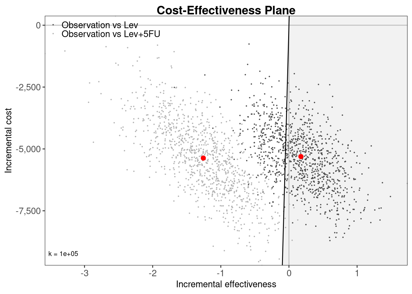
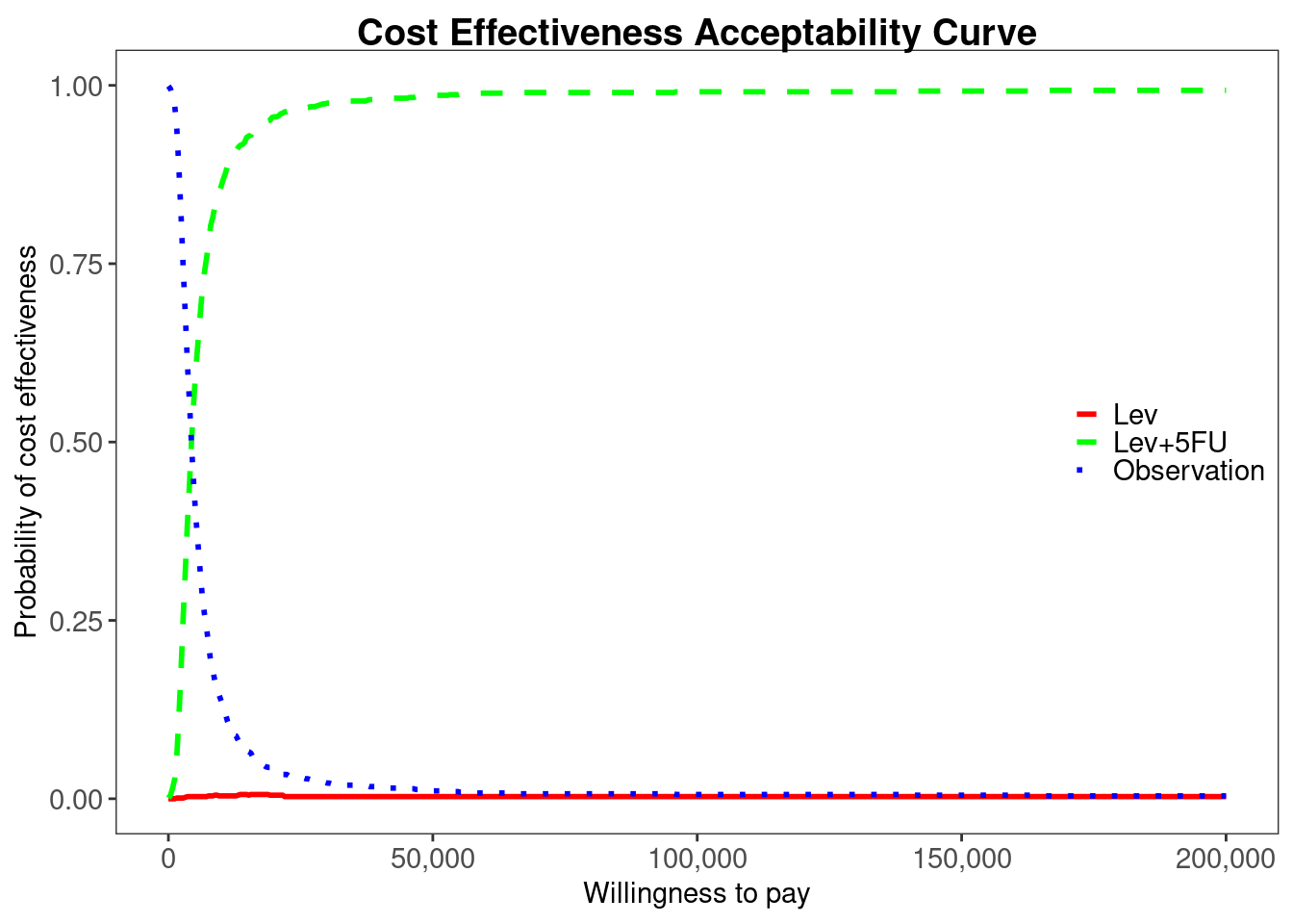
BCEA
As the bcea() function expects effects e and costs c to be n_samples by n_treatments it is necessary to transpose the total_qalys and total_costs matrices using the t() function.
9.7 Discussion
In this chapter, we have moved from basic concepts of Markov modelling to the full implementation in R of a probabilistic time-inhomogeneous Markov model. Our application throughout was a comparison of three interventions for post-surgery adjuvant therapy for colon cancer (Section 9.2). To aid generalisation and clarify concepts, we used base R for the core modelling. The first level of complexity was a deterministic time-homogeneous Markov model in Section 9.4, where in Section 9.4.2 we described the use of matrix multiplication to update a cohort vector using transition matrices. The next level was a deterministic time-inhomogeneous Markov model in Section 9.5, where the key change was to add a cycles dimension to the transition matrices. The possibility of state costs or state utilities also changing with time was covered by including a cycles dimension in state_costs in Section 9.5.3, with the same approach applicable to state_utilities. The final level of complexity was to make the time-inhomogeneous Markov model probabilistic in Section 9.6. This added a dimension for samples to the transition matrices, state costs, and state utilities, and used suitable distributions to represent uncertainty in these input parameters. The key change to the model code was to add a further for loop over samples in Section 9.6.3.
The code we have provided is tailored to the 4-state Markov model for colon cancer illustrated in Figure 9.2 (a) but is generalisable to any model structure and parameters. The number and names of states can be modified by changing n_states and state_names, and then by appropriately defining transition_matrices, state_costs, and state_qalys. The Markov loops for deterministic time-homogeneous, deterministic time-inhomogeneous, and probabilistic time-inhomogeneous updating of the Markov trace would remain unchanged, as would the code for calculating total costs and QALYs. A probabilistic time-homogeneous model can also be developed by adapting the code in Section 9.4 to include samples, or the code in Section 9.6 to remove cycles.
If adapting the code in Section 9.4, we would first add n_samples dimensions to the input parameters represented by transition_matrices_homogeneous, state_costs, state_qalys, and treatment_costs, and define appropriate distributions for their values. We would also add n_samples dimensions to the output objects Markov_trace_homogeneous, cycle_costs, cycle_qalys, total_costs, and total_qalys. Finally we would add an extra for loop over n_samples to the Markov update code in Box 9.9 and the total costs and QALYs calculation in Box 9.13. This would be a useful exercise for anyone new to Markov modelling in R.
Several survival distributions were used for the transition probabilities in the colon cancer Markov model, and were incorporated using the transformations in Section 9.3.2. A Gompertz distribution was used for background mortality, a log-logistic mixture cure was used for recurrence, and an exponential distribution was used for cancer mortality. These could be changed to other standard parametric distributions, piecewise constant exponential models, fractional polynomials, splines, or other survival models described in Chapter 7. Given the extensive coverage of survival analysis elsewhere in this book, we did not describe their conduct and limited our consideration to how to use such models for transition probabilities in Markov models.
We have noted the extensions to Markov modelling that will be described in Chapter 11 on general multistate modelling. These include moving from cohort to individual level, from discrete-time to continuous-time, and from a Markov assumption to the semi-Markov assumption. This later chapter utilises the hesim package that could be used to implement the various Markov models we have described. Full individual modelling using discrete event simulation is described in Chapter 12. Discrete event simulations may be more appropriate if events better describe the disease than states, if individual outcomes are heterogeneous, or if individual disease history has a complex relationship to future disease course. Conversely, Chapter 8 described decision tree models which may be more appropriate than Markov or multistate models, or indeed discrete event simulations, if the time horizon is short and there are few repeat events to model.
Our application assumed that a single trial was available to inform transition probabilities. If multiple studies are available, meta-analysis and network meta-analysis, as described in Chapter 10 may be more necessary. These could estimate log hazard ratios or log odds ratios that can be applied to rates and transformed to transition probabilities using the methods of Section 9.3.2. The total costs and QALYs estimated by our probabilistic Markov model could be used to estimate the value of information, and this topic is described in Section 1.8. Furthermore, R Shiny could be used to add a graphical user interface to our Markov models, as described in Chapter 14.
We have omitted several potentially important topics in discrete-time cohort Markov modelling. One such topic is the use of deterministic sensitivity analysis (DSA). This is a deterministic approach to exploring parameter uncertainty where parameters are set to their upper and lower limits (e.g., the upper and lower limits of their 95% confidence interval, or their maximum and minimum values) and the ICER or other model output recalculated. Other parameters are held constant at their point estimates so that only uncertainty in the target parameter is captured. This could be implemented manually using the deterministic code in Section 9.4 or Section 9.5. Structural uncertainty can include uncertainty in the included states, allowed transitions, or survival distributions, or any uncertainty that can not be parametrised (Jackson et al., 2011). This could be explored in a similar to manner to DSA with alternative structures implemented, the ICER or other output recalculated, and then compared to the base case. Discrepancy or constraint approaches to structural uncertainty could also be implemented using the code we have provided, by simply changing the input parameter distributions on transition probabilities, costs, and utilities (Strong et al., 2012; Thom et al., 2017). Related to structural uncertainty is the use of tunnel states to relax the Markov assumption. These could capture variation with time of the mortality rate in the Recurrence state by splitting Recurrence into, for example, “Recurrence cycle 1”, “Recurrence cycle 2”, “Recurrence cycle 3”, etc. Patients would be assumed to transition from to the subsequent state each cycle, with the transition rate to Dead (Cancer) changing. These can be implemented by increasing n_states and specifying elements of the transition matrices to be 1 minus the risk of (cancer or all-cause) death so that transitions to subsequent tunnel states must occur each cycle.
We have not touched on optimisation of our code. However, for loops are known to be inefficient and could be optimised through judicious use of vectorisation. Further efficiency could be gained by implementing the core Markov loop in the low-level, and high-speed, C++ programming language using the Rcpp package.
Our application is historical but nonetheless represents an interesting exercise in comparative modelling. Using all three approaches we found that Levamisole was dominated by Observation, with both higher costs and lower QALYs. More interesting was the variation in the ICER for Levamisole and fluorouracil compared to Observation. This was $21,797/QALY using the deterministic time-homogeneous model, $4,357/QALY using the deterministic time-inhomogeneous model, and $4,306/QALY using the probabilistic time-inhomogeneous model. This would suggest that the variation of parameters with time was a more important element to capture than the parameter uncertainty. The colon example is further explored in Chapter 11 and Chapter 12.
In summary, we have provided generalisable R code for cohort discrete-time Markov models, which can be extended to other state structures and other survival models on transition rates, to incorporate network meta-analyses, and to explore parameter and structural uncertainty. Optimisation by removing for loops should be considered if runtime becomes impractical. Decision trees, general multistate, and discrete event simulation models provide alternative modelling approaches and we refer the interested reader to the relevant chapters of this book.