| Parameter simulations | Expected utility | VoI analysis | ||||||
|---|---|---|---|---|---|---|---|---|
| Sims | \(\theta_1\) | \(\theta_2\) | \(\ldots\) | \(\theta_Q\) | \(\text{NB}_1(\boldsymbol{\theta})\) | \(\text{NB}_2(\boldsymbol{\theta)}\) | \(\text{NB}^*(\boldsymbol{\theta})\) | \(\text{OL}(\boldsymbol{\theta})\) |
| 1 | 0.58 | 0.38 | \(\ldots\) | 0.42 | 77480 | 67795 | 77480 | 9685 |
| 2 | 0.51 | 0.02 | \(\ldots\) | 0.08 | 87165 | 106535 | 106535 | 0 |
| 3 | 0.61 | 0.14 | \(\ldots\) | 0.06 | 58110 | 38740 | 58110 | 19370 |
| 4 | 0.2 | 0.73 | \(\ldots\) | 0.73 | 77480 | 87165 | 87165 | 0 |
| \(\ldots\) | \(\ldots\) | \(\ldots\) | \(\ldots\) | \(\ldots\) | \(\ldots\) | \(\ldots\) | \(\ldots\) | \(\ldots\) |
| \(S=1000\) | 0.03 | 0.2 | \(\ldots\) | 0.56 | 48425 | 87165 | 87165 | 0 |
| Average: | 72365.35 | 77403.49 | 91192.02 | 13788.53 | ||||
12 Value of information
12.1 Introduction
We have seen throughout the many examples in the previous chapters that a fundamental component of the HTA process is the characterisation and full analysis of the impact of uncertainty in the model parameters on the decision-making. As mentioned in Note 4.4 in Section 4.3.3, this exercise cannot be made purely on probabilistic terms, because doing so (e.g. by using the CEACs) would fail to account for the potential payoffs associated with the decision.
In other words, there may be situations in which large uncertainty in the model parameters (and thus, potentially, on the probability that a given intervention is deemed to be the most cost-effective) is associated with very limited consequences. Similarly, it is possible that situations that, at face value, do not look highly uncertain may hide dire consequences – the (admittedly silly) example in Note 4.4 is a point in case.
These considerations suggest that, in fact, the process of “uncertainty analysis” as defined in Section 4.3 is a bit more complicated and involves more nuanced aspects. These can be better understood and more efficiently tackled under the framework of “Value of Information” (VoI) analysis (originally devised in Howard, 1966), an increasingly popular method in health economic evaluations.
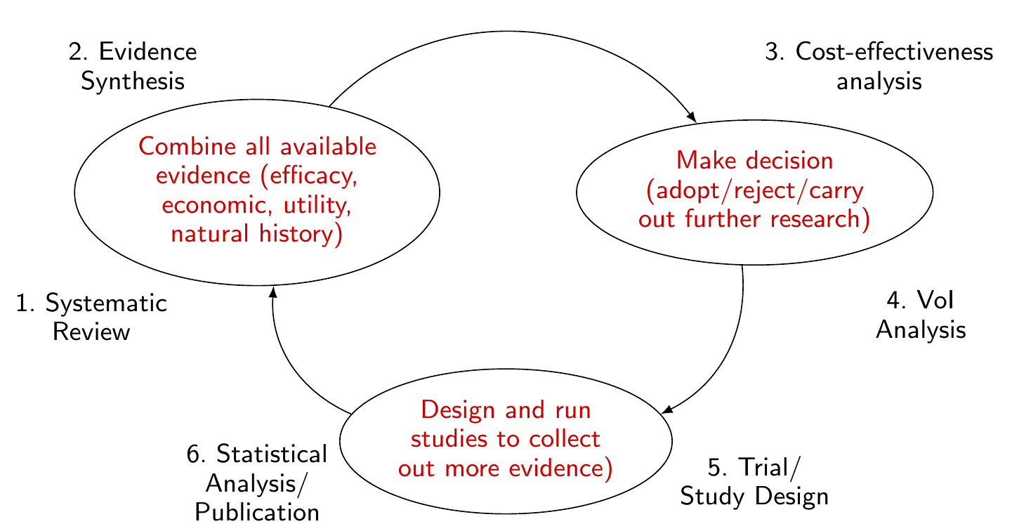
More specifically, the process can be depicted graphically as in Figure 12.1, where the main point is the suggestion of the cyclical nature and evidence is hardly ever definitive. At the point of initiating a new HTA evaluation, researchers must look into the existing evidence basis, e.g. through a systematic review. All the available evidence must be combined (e.g. using the processes described in Chapters 6 and 7) to feed into the main cost-effectiveness analysis, based on current evidence. This determines the decision, which is not just binary in terms of adopt/reject, but also involves through the uncertainty analysis the explicit option of collecting more information and carrying out more research.
This is the stage in which the analysis of the “value of information” plays a fundamental role, as we will show in the rest of this chapter. In particular, this should drive the research priorities, in terms of what is the best design to collect new information and which quantities to target to reduce uncertainty. This leads to an increment in the evidence basis, which should be accounted for when the process can start over with a new systematic review. This characterisation suggests that the overall HTA process is inherently Bayesian – recall the mantra of Lindley (1972), as discussed in Section 1.2.2.
Heath et al. (2024) is the most recent and comprehensive textbook on the use of VoI in healthcare. The companion voi package (Jackson and Heath, 2024) can be used to perform the actual calculations – cfr. also the package website https://chjackson.github.io/voi/articles/book.html for code to replicate the examples discussed in Heath et al. (2024).
12.2 Basic ideas
Generally speaking, at the point of considering the conduct of a new study before firmly committing to a new intervention, the main expectation is that the new evidence will contribute to reducing – or, in an ideal world, fully eliminating – uncertainty in at least a subset of the model parameters.
When updating the cost-effectiveness analysis, on the basis of the new evidence that becomes available, we may find that the optimal decision has changed – we may have thought that \(t=2\) was the most cost-effective treatment on the basis of the original evidence, but now \(t=1\) is deemed to be better value for money. In this case, we would generate a change in the monetary net benefit (MNB – cfr. Equation 4.3 and Section 4.2) through the acquisition of the new evidence.
Conversely, we may see no difference in the optimal decision-making before and after the collection of the new data – in that case, we would have produced no increase in the MNB. The expected VoI can be quantified by the average gain in MNB from the collection of new data.
In general, VoI measures are always expressed as something like \[ \begin{aligned} \text{VoI measure} = & \;\text{Value of an \textit{idealised} decision-making process} \;-\; \\ &\; \text{Value of the \textit{current} decision-making process}. \end{aligned} \tag{12.1}\]
NoteVoI analysis in practice
The nature of VoI analysis intrinsically considers a hypothetical future scenario in which, somehow, we are able to gain more information in order to reduce or eliminate uncertainty in some or all the model parameters. In practice, this is most likely an idealised situation, which may be impossible to obtain. More importantly, we do this analysis before we get to see any new data – the point of VoI is exactly to quantify the potential benefits of running the extra analysis prior to actually investing the money to do it!
For this reason, in addition to performing uncertainty analysis, VoI is used as a tool for research prioritisation – the idea that we can identify what specific parameters we should investigate out of the many that characterise our model. Thus, when performing VoI, there are two important consequences.
Firstly, any VoI measure in itself is only meaningful in expectation – it is the various forms of Expected Value of Information that are helpful to us. This is because we do not have the actual new data yet, but we can try and quantify what we expect to gain from them, if we are actually able to collect them.
As a consequence, Equation 12.1 is meaningful (and drive how VoI measures are constructed) when we take relevant expectations on both sides. The second term on the right-hand side of Equation 12.1 is represented by \[ \max_t \text{E}_{\boldsymbol\theta} \left[\text{NB}_t(\boldsymbol\theta)\right], \] which determines the treatment that, given current evidence, is associated with the highest expected utility. The first term depends on the idealised process, as we clarify in Equations 12.2, 12.3 and 12.9. In all cases, however, it involves a suitable expectation of a relevant maximisation – essentially flipping around the order of the two operations, in comparison to the term related to the current decision-making process.
The second important point to make about VoI practical calculation is that it is essentially a predictive measure (see for instance the analysis in Example 3.1 in Section 3.2). In other words, we use the information arisen from the current analysis/modelling to obtain this expectation.
Even more specifically, this means that the basis for the computation of any measure of VoI is in the uncertainty analysis for the current model (see Section 4.3 and Table 4.1, in particular).
In terms of interpretation, the main complexity of Equation 12.1 is that there is no natural upper bound. VoI measures are positive (because, in the worst-case scenario, there is no gain in MNB), but it is not possible to define an absolute scale and thus it is hard to assess directly “how low is a low VoI”.
This suggests that we must take other factors into account – for instance the actual cost of acquisition of the new evidence (e.g. the conduct of a confirmatory RCT). In addition, we should consider carefully what is the (subgroup in the) population that would be mostly affected both by the technology under evaluation and by the evidence collected. Finally, another important consideration is about the time horizon over which the new intervention/evidence are assumed to bear an impact. We return to these points particularly in Section 12.5.
In addition, from the pragmatic point of view, there are important computational and modelling issues, which have for a very long time impaired the establishment of VoI as a principled and applicable methodology to perform uncertainty analysis in HTA. These have been largely overcome in recent times, with a large body of literature devoted to devising methods for fast and reliable computation of various VoI measures, which we review particularly in Section 12.4 and Section 12.5.
12.3 Expected value of perfect information
There are, roughly speaking, three different measures for VoI. The simplest (and in many ways less useful) is the Expected Value of Perfect Information (EVPI).
We can think of this as a highly idealised scenario in which we are able to collect evidence that can completely remove all uncertainty in all the model parameters. Clearly, this is pretty much an impossibility, as it would amount to a study with infinite sample size to learn perfectly all the relevant parameters \(\boldsymbol\theta\). Despite this, the EVPI is a useful measure to grasp the basic concept of VoI and it can be proved that it places an upper limit to the amount of money that we should be willing to invest to improve the decision-making process.
One effective way of thinking about this problem is to consider a PSA table, such as that described in Table 4.1, or, more specifically, the one shown in Table 12.1. Here, we assume that our economic model is characterised by \(Q\) parameters \(\boldsymbol\theta=(\theta_1,\ldots,\theta_Q)\) and that we are able to produce a MCMC analysis in which we obtain \(S=1000\) simulations from the posterior distribution \(p(\boldsymbol\theta\mid \boldsymbol{y})\), for some suitable data \(\boldsymbol{y}\). For each simulated value of the parameters, we can construct the net benefit associated with two relevant options, a status quo \(t=1\) and the new intervention \(t=2\). Averaging over the \(S\) simulations allows us to compute the overall expected utilities, which are presented at the bottom of Table 12.1.
We can define \[ \begin{aligned}[t] \text{EVPI}& = \text{E}_{\boldsymbol\theta}\left[\max_t \text{NB}_t(\boldsymbol\theta) \right] - \max_t \text{E}_{\boldsymbol\theta} \left[\text{NB}_t(\boldsymbol\theta)\right] \\ & = \text{E}_{\boldsymbol\theta}\left[\text{NB}^*(\boldsymbol\theta) \right] - \mathcal{NB}^*, \end{aligned} \tag{12.2}\] where, for each PSA simulation \(s=1,\ldots,S\) in Table 12.1, the quantity \[\text{NB}^*(\boldsymbol\theta)=\max_t \text{NB}_t^{(s)}(\boldsymbol\theta)\] is the row-wise maximum net benefit (i.e. the values typeset in italics in each row) and \(\mathcal{NB}^*\) is defined in Equation 4.5. In this example, the EVPI amounts to \(91192.02-77403.49=13788.53\).
In terms of Table 12.1, for each PSA simulation \(s=1,\ldots,S\), the Opportunity Loss \[ \text{OL}(\boldsymbol\theta)=\text{NB}^*(\boldsymbol\theta)-\text{NB}_{t^*}^{(s)}(\boldsymbol\theta) \] is the row-wise difference between the maximum net benefit \(\text{NB}^*(\boldsymbol\theta)\) and the net benefit for the overall most cost-effective intervention, \(t^*=\arg\max \text{E}_{\boldsymbol{\theta}} \left[\text{NB}_t(\boldsymbol\theta)\right]\), which in this case is \(t=2\) – as is possible to see in the last row of Table 12.1, where the overall expected utilities are \(\mathcal{NB}_2=77403.49>\mathcal{NB}_1=72365.35\) (cfr. also Table 4.1).
Interestingly, \[ \begin{aligned} \text{E}_{\boldsymbol\theta}\left[\text{OL}(\boldsymbol\theta)\right] & =\text{E}_{\boldsymbol\theta}\left[\text{NB}^*(\boldsymbol\theta)-\text{NB}_{t^*}(\boldsymbol\theta)\right] = \text{E}_{\boldsymbol\theta}\left[\text{NB}^*(\boldsymbol\theta)\right]-\text{E}_{\boldsymbol\theta}\left[\text{NB}_{t^*}(\boldsymbol\theta)\right] \\ & = \text{E}_{\boldsymbol\theta}\left[\max_t \text{NB}_t(\boldsymbol\theta)\right] - \max_t \text{E}_{\boldsymbol\theta}\left[\text{NB}_t(\boldsymbol\theta)\right] \end{aligned} \] and thus Equation 12.2 can be expressed equivalently as the average \(\text{OL}(\boldsymbol\theta)\) – cfr. Table 12.1.
A typical EVPI analysis can be summarised against the grid of values for the willingness-to-pay, \(k\), as in Figure 12.2.
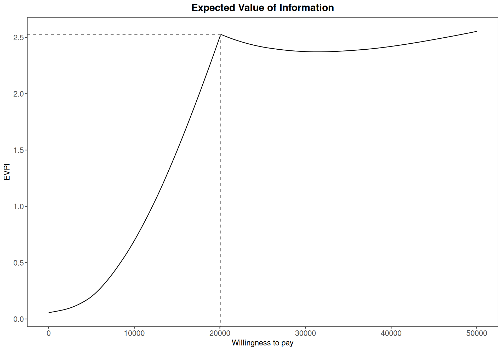
Figure 12.2 shows a “kink” at around \(k=20100\), which indicates the “break-even point” (BEP), i.e. the value of the willingness to pay in correspondence of which the optimal decision changes. This explains why the EVPI is effectively a combination of two separate functions – one, increasing quite steeply and leading up to the BEP and the other, showing a much flatter shape, after the BEP. Generally speaking, expected VoI curves typically show behaviours such as this and may have multiple change-points, when the optimal decision changes over the range of willingness-to-pay thresholds selected.
In Figure 12.2, the \(y\)–axis represents the monetary value of expected information – in other words, the maximum amount that we should be prepared to pay to buy new data to completely eliminate the uncertainty on all the model parameters. In this particular case, this is at most £2.5 per individual, which is obviously very small, indicating that the impact of uncertainty in the decision-making process is probably negligible and thus we can use the current data to make a decision.
As mentioned above, however, in general it is a bit more complicated to interpret this value, because the absolute magnitude must be put in relation with the cost of acquisition of the new evidence. For instance, if \(\text{EVPI}= \text{£} 1000000\), we may argue that there is large value in reducing uncertainty and therefore we should consider deferring the decision until we get more data. But of course this depends on how much would the actual data-generating process cost – if, say, we could design a suitable trial at the cost of £\(3000000\), then we would be in fact losing a substantial amount of money by doing it!
We return to this point more specifically in Section 12.5.1.
12.4 Expected value of partial perfect information
One of the ways in which we can relax the frankly unrealistic assumptions of the EVPI, i.e. that we can get all the information we need for all the model parameters, is to realise that, even if it were possible to completely eliminate the uncertainty, there may be some parameters that matter more to us. In other words, we can think of partitioning the vector of model parameters as \(\boldsymbol\theta = (\boldsymbol\phi,\boldsymbol\psi)\), where \(\boldsymbol\phi\) is the subset of the “parameters of interest” (often termed as “focal”), while \(\boldsymbol\psi\) are the “remaining” or “nuisance” parameters.
The former may include quantities such as the prevalence of a disease, HRQL measures or length of stay in hospital, while the latter may be variables such as the cost of treatment with other established medications. The main idea here is that for some of the parameters, the uncertainty may just be beyond our control – for instance, if the cost of acquisition is not fixed, but determined by legal regulations, which we cannot modify.
In this particular scenario, the interest is in quantifying the value of gaining more information on \(\boldsymbol\phi\), while leaving current level of uncertainty on \(\boldsymbol\psi\) unchanged. The relevant VoI measure is referred to as Expected Value of Partial Perfect Information (EVPPI) and is defined as \[ \text{EVPPI}= \text{E}_{\boldsymbol\phi}\left[\max_t\text{E}_{\boldsymbol\psi\mid\boldsymbol\phi}[\text{NB}_t(\boldsymbol\theta)]\right]-\max_t \text{E}_{\boldsymbol\theta}[\text{NB}_t(\boldsymbol\theta)]. \tag{12.3}\] Intuitively, we think of this process along those lines: if we were truly able to learn perfectly the value of \(\boldsymbol\phi\), while leaving \(\boldsymbol\psi\) at the current uncertainty, the decision making process would be effected by looking at \(\max_t\text{E}_{\boldsymbol\psi\mid\boldsymbol\phi}[\text{NB}_t(\boldsymbol\theta)]\), i.e. we would first compute the relevant expected utility associated with each treatment option and then we would maximise it to determine the most cost-effective option.
Of course, we cannot learn \(\boldsymbol\phi\) with absolute certainty and thus the idealised decision process is in fact obtained by taking the average (with respect to the relevant parameters, \(\boldsymbol\phi\)) of this quantity. In line with Equation 12.1, we need to compare this with the current decision-making process, which is again defined as \(\max_t \text{E}_{\boldsymbol\theta}[\text{NB}_t(\boldsymbol\theta)]\).
In all but really trivial models, \(\max_t\text{E}_{\boldsymbol\psi\mid\boldsymbol\phi}[\text{NB}_t(\boldsymbol\theta)]\) is the element that contributes to the high computational complexity of this operation, because it involves a maximisation of an expectation, i.e. nested (typically complex and highly non-linear) integral operations.
For this reason, while the theoretical underpinning of the EVPPI is just as old as that of the much simpler EVPI, until very recently (particularly with the key contributions of Strong et al., 2014; and Heath et al., 2016) it has been virtually impossible to perform calculations for the EVPPI in realistically complex models.
12.4.1 Computing the EVPPI through brute force nested Monte Carlo
The simplest way of computing the EVPPI is through “brute force” and applying nested Monte Carlo integration. This assumes that we first simulate a large number of values, say \(S_\phi\) from the marginal distribution of the parameters of interest, \(\boldsymbol\phi\). Then, conditionally on each of these values, we simulate a further layer of nested simulation, say \(S_\psi\) values, from the conditional distribution \(p(\boldsymbol\psi\mid\boldsymbol\phi=\boldsymbol\phi^{(s)})\), for each \(s=1,\ldots,S_\phi\).
For instance, assuming there are only two relevant interventions \(t=1,2\) and thus \(\text{IB}(\boldsymbol\theta)=\text{NB}_2(\boldsymbol\theta)-\text{NB}_1(\boldsymbol\theta)\), we can use these \(S_\phi \times S_\psi\) simulations to characterise the distribution of the expcected incremental benefit, as in Figure 12.3 (a).
Here, the ticks along the \(x\)–axis indicate the \(S_\phi\) simulated values from the marginal distribution \(p(\boldsymbol\phi)\). For each of these values, the dots are the \(S_\psi\) simulations from the conditional distribution \(p(\boldsymbol\psi\mid\boldsymbol\phi=\boldsymbol\phi^{(s)})\), which can be used to determine the expected incremental benefit, shown along the \(y\)–axis as the crosses. The decision-making process based on this representation would imply that whenever \(\text{E}\left[\text{IB}(\boldsymbol\theta)\right]>0\) then the new treatment \(t=2\) would be deemed as more cost-effective, while in correspondence of values for \(\boldsymbol\phi\) that are associated with \(\text{E}\left[\text{IB}(\boldsymbol\theta)\right]<0\), then the status quo \(t=1\) would be preferred.
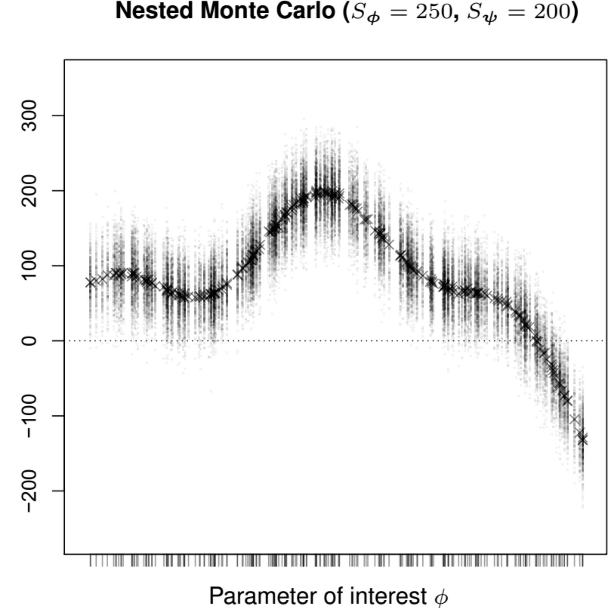
While this approach is reasonably easy to follow, it has the major drawback of being utterly inefficient, because in order to fully characterise both the marginal and the conditional distributions of interest, we will need a very large number of simulations for both layers – a typical recommendation is that \(S_\phi\) and \(S_\psi\) should be in the order of 10 000 (Brennan et al., 2007), leading to a very large number of overall simulations.
Note 12.1: Non-additivity of the EVPPI
Another case in which the computation of the EVPPI is much simplified is when we consider a single parameter of interest, e.g. \(\boldsymbol\phi=\theta_1\) and thus \(\boldsymbol\psi=(\theta_2,\ldots,\theta_Q)\). In this case, we can probably use the nested MC approach discussed above; however, one additional complexity is that the EVPPI is a non-additive measure, i.e. in general \[\text{EVPPI}({\phi_1,\phi_2})\neq \text{EVPPI}({\phi_1}) + \text{EVPPI}({\phi_2}).\]
Thus, the value of learning about multiple variables together can be higher, lower, or equal to the sum of their individual EVPPI values, due to potentially high dependencies in the decision-making process and interactions between uncertainties.
For this reason, while the univariate EVPPI analysis may be a helpful starting point, we should not rely on this if we are truly interested in groups of parameters.
12.4.2 Regression-based approximation to the EVPPI
Strong et al. (2014) introduced the idea of framing this problem within the context of non-linear regression. In this setup, we can consider the PSA simulations for the important parameters as a set of \(Q_{\boldsymbol\phi}\) “observed covariates” \(\boldsymbol{X}\), while the resulting PSA simulations for the net benefit for each treatment considered as a vector of “observed outcomes” \(\boldsymbol{y}\). Table 12.2 shows this situation using a fictional PSA simulation.
| Outcome \(\boldsymbol{y}\) | Covariates \(\boldsymbol{X}\) | Nuisance parameters | |||||||
|---|---|---|---|---|---|---|---|---|---|
| Sims | \(\text{NB}_t(\boldsymbol{\theta)}\) | \(\phi_1\) | \(\phi_2\) | \(\ldots\) | \(\phi_{Q_\phi}\) | \(\psi_1\) | \(\psi_2\) | \(\ldots\) | \(\psi_{Q_\psi}\) |
| 1 | 41628 | 0.58 | 0.82 | \(\ldots\) | 0.59 | 2.68 | 0.77 | \(\ldots\) | 0.71 |
| 2 | 41628 | 0.31 | 0.08 | \(\ldots\) | 0.20 | 1.77 | 0.06 | \(\ldots\) | 0.04 |
| 3 | 34690 | 0.23 | 0.31 | \(\ldots\) | 0.23 | 0.84 | 0.08 | \(\ldots\) | 0.30 |
| 4 | 62442 | 0.58 | 0.22 | \(\ldots\) | 0.77 | -0.65 | 0.34 | \(\ldots\) | 0.06 |
| \(\ldots\) | \(\ldots\) | \(\ldots\) | \(\ldots\) | \(\ldots\) | \(\ldots\) | \(\ldots\) | \(\ldots\) | \(\ldots\) | \(\ldots\) |
| \(S\) | 48566 | 0.25 | 0.49 | \(\ldots\) | 0.73 | -1.38 | 0.55 | \(\ldots\) | 0.52 |
Notice that in this particular case, we slightly abuse the wording of our problem, since the “data” used to run the regression model are not really observed: rather, they are simulations based on the current economic model, reflecting the current state of uncertainty about the model inputs.
In a nutshell, the idea is to model \[ \begin{aligned}[b] \text{NB}_t(\boldsymbol\theta) & = \text{E}_{\boldsymbol\psi\mid\boldsymbol\phi}[\text{NB}_t(\boldsymbol\theta)] + \varepsilon \\ & = g(\boldsymbol\phi) + \varepsilon, \end{aligned} \tag{12.4}\] with \(\varepsilon \sim \text{Normal}(0,\sigma^2_\varepsilon)\) and where \(g(\boldsymbol\phi)\) is an unknown, non-linear function that can be used to approximate as best as possible the unknown conditional expectation \(\text{E}_{\boldsymbol\psi\mid\boldsymbol\phi}[\text{NB}_t(\boldsymbol\theta)]\) – note that when taking the conditional expectation, the net benefit only depends on \(\boldsymbol\theta\) through the subset \(\boldsymbol\phi\) and hence so does the function \(g(\cdot)\).
In comparison to the brute force approach, this can be much more efficient, because we only use a relatively small number of “data points”, i.e. the \(S\) PSA simulations, which are usually in the order of a few thousands. Of course, we can extend the size of the MCMC simulations from the model parameters that we use to construct Table 12.2, but we would generally still require a much smaller sample size than in the nested MC case.
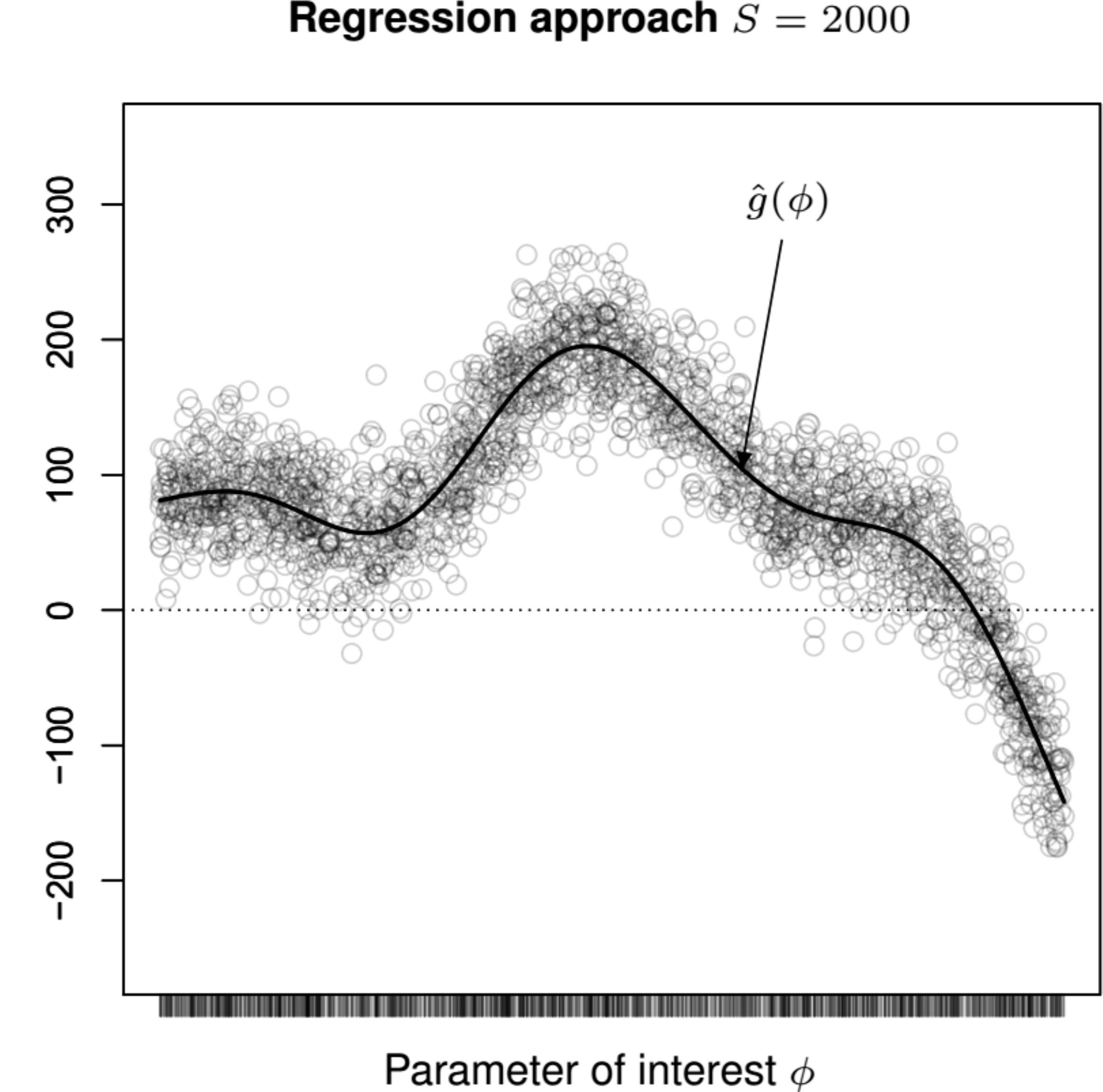
The main idea is shown graphically in Figure 12.3 (b): here, the circles represent the \(S\) PSA simulations from the distribution of \(\boldsymbol\phi\) – notice that, in this case, we consider only \(S=2000\), as opposed to the \(S_\phi\times S_\psi=250\times 200 = 50000\) nested MC simulations used in the brute force approach. We feed these “data points” to the regression model to estimate the function \(\hat{g}_t\left(\boldsymbol\phi^{(s)}\right)\), which in turn can be used to approximate Equation 12.3 using the \(S\) PSA simulations as \[ \text{EVPPI}\approx\frac{1}{S}\sum_{s=1}^S \max_t {\textstyle\hat{g}_t\left(\boldsymbol\phi^{(s)}\right)}- \max_t \frac{1}{S}\sum_{s=1}^S {\textstyle \hat{g}_t\left(\boldsymbol\phi^{(s)}\right)}. \]
Obviously, the main complexity of the regression-based approach is to effectively retrieve the underlying unknown, non-linear relationship that characterises the function \(g(\cdot)\). Strong et al. (2014) and Heath et al. (2016) suggest either the use of Generalised Additive Models (GAMs, Hastie and Tibishirani, 1990; and Wood, 2017), or extensions based on Gaussian Process (GP) regression (Williams and Rasmussen, 2006), as very efficient options.
We quickly review both below, while Heath et al. (2024, specifically in sec. 3.4) present extended R code to use GAMs or GPs to compute the EVPPI in applied examples, using the voi package.
Generalised additive models
For each treatment option \(t=1,\ldots,T\), GAMs define \[ g_t(\boldsymbol\phi)=\sum_{q=1}^{Q_{\boldsymbol\phi}} {\textstyle h_t\left(\phi_{q}^{(s)}\right)}, \tag{12.5}\] where, again, \(Q_{\boldsymbol\phi}\) is the number of important parameters; \(\phi_{q}^{(s)}\) is the \(s-\)th PSA simulation for the \(q-\)th important parameter; and the functions \(h_t(\cdot)\) are piecewise polynomials, whose degree defines the smoothness of the \(g_t(\cdot)\).
Much as splines (see Section 8.5.1), GAMs can be implemented as a frequentist or a Bayesian model. When using GAMs, the package voi is based on the implementation developed in the R package earth (Milborrow, 2011), which is in fact a frequentist analysis.
The “vanilla” implementation of GAMs uses one-dimensional splines for each parameter, which, as mentioned in Note 12.1 above, can be overly restrictive, particularly when parameters are highly correlated. To overcome this limitation, we can extend the formulation in Equation 12.5 to include interaction terms. This is generally very powerful, but tends to explode the computational complexity of the model, meaning that estimates should be based on a much larger PSA sample, thus reducing the advantages of the regression-based approach – see also Heath et al. (2024) and Baio et al. (2025, pp. 113–124) for a much more technical and extensive description.
For this reason, when the number \(Q_{\boldsymbol\phi}\) of parameters included in \(\boldsymbol\phi\) is sufficiently “large” say, above 5, GP regression can be used as an efficient alternative (Strong et al., 2014; Heath et al., 2016; Baio et al., 2025).
Gaussian Process regression
The GP regression approach starts by considering for each treatment or intervention under consideration a multivariate regression model \[ \left(\text{NB}_t^{(1)}(\boldsymbol\theta), \text{NB}_t^{(2)}(\boldsymbol\theta),\ldots,\text{NB}_t^{(S)}(\boldsymbol\theta)\right) \sim \text{Normal}(\boldsymbol{H} \boldsymbol\beta, \boldsymbol\Sigma + \sigma_\varepsilon^2\boldsymbol{I}), \tag{12.6}\] where \[ \boldsymbol{H} =\left( \begin{array}{c c c c} 1 & \phi_{1}^{(1)} & \cdots & \phi_{Q_{\phi}}^{(1)} \\ 1 & \phi_{1}^{(2)} & \cdots & \phi_{Q_{\phi}}^{(2)} \\ \vdots& & \ddots\\ 1 & \phi_{1}^{(S)} & \cdots & \phi_{Q_{\phi}}^{(S)} \\ \end{array}\right) \tag{12.7}\] is a “design matrix” and \(\boldsymbol\phi^{(s)}\) are the values of the \(s\)-th PSA simulations for the subset of important parameters, \(\boldsymbol\phi\). The quantity \(\sigma_\varepsilon^2\) is the residual variance from the regression construction, while \(\boldsymbol{I}\) is a \((S\times S)\) identity matrix and \(\boldsymbol\beta=(\beta_0,\ldots,\beta_{Q_{\phi}})\) is a vector of length \((Q_{\phi}+1)\) of regression coefficients used to model the linear relationship between \(\boldsymbol\phi\) and \(\text{E}_{\boldsymbol\psi\mid\boldsymbol\phi} [\text{NB}_t(\boldsymbol\theta)]\).
In a GP regression, the linear structure is rendered flexible by constructing the covariance matrix \(\boldsymbol\Sigma\) in terms of a covariance function \(\mathcal{C}(r,s)\), which can be used to describe the joint variability of any two “observed” points \(\text{NB}_t^{(r)}(\boldsymbol\theta)\) and \(\text{NB}_t^{(s)}(\boldsymbol\theta)\) – in our case, these are two PSA simulations for the net benefit.
The standard implementation of the GP regression model considers a squared exponential covariance function \[ \mathcal{C}_{\textrm{Exp}}(r,s) = \sigma^2 \exp\left[\sum_{q=1}^{Q_\phi} \left(\frac{\phi_{q}^{(r)}-\phi_{q}^{(s)}}{\delta_q} \right)^2\right]. \tag{12.8}\] Here, \(\sigma^2\) is the GP marginal variance, while the \(q-\)th element of the vector \(\boldsymbol\delta=(\delta_1,\delta_2,\ldots,\delta_{Q_{\boldsymbol\phi}})\) defines the “smoothness” of the relationship between two net benefit values with “similar” values for each of the \(q-\)th important parameter \(\boldsymbol\phi_q\).
This model is more naturally Bayesian and we can specify a full set of prior distributions, including for the \((2Q_{\boldsymbol\phi}+3)\) hyperparameters \((\boldsymbol\beta,\boldsymbol\delta,\sigma,\sigma_{\varepsilon})\). This, however, can still be very computationally intensive and thus, in practice, the estimates are obtained through numerical optimisation and, possibly, conjugate modelling (Strong et al., 2014).
Borrowing from the context of spatial and spatio-temporal modelling and Integrated Nested Laplace Approximation (INLA), Heath et al. (2016) suggest a revised version of the GP regression to speed up the computations – see for instance Blangiardo and Cameletti (2015); or Gómez-Rubio (2020), among others, as well as Section 3.1.2 for more details in INLA.
In a nutshell, the main idea is to re-formulate the regression model as \[ \left(\text{NB}_t^{(1)}(\boldsymbol\theta), \text{NB}_t^{(2)}(\boldsymbol\theta),\ldots,\text{NB}_t^{(S)}(\boldsymbol\theta)\right) \sim \text{Normal}(\boldsymbol{H} \boldsymbol\beta + f(\omega), \sigma_\varepsilon^2\boldsymbol{I}), \] in terms of the linear predictor \(\boldsymbol{H} \boldsymbol\beta\) and a “spatially structured” effect \(f(\omega)\), which absorbs all the non-linearity and correlation among the parameters in \(\boldsymbol\phi\). This spatial effect can be estimated efficiently using a combination of Stochastic Partially Differential Equations (SPDE – see Gómez-Rubio, 2020; Krainski et al., 2019; Lindgren et al., 2011 for more technical descriptions and insights) and INLA.
Intuitively, the main advantage of this process is that we can use a simple linear component and augment the model using, effectively, a specific random effect to obtain a non-linear, flexible estimate for the function \(g_t(\cdot)\).
NoteSpatial modelling and the EVPPI
Technically speaking, the spatial structure associated with \(\omega\) implies that it should have a bi-dimensional nature – this is what happens in typical geostatistical analysis in which we model the correlation between points in the 2-d geographical space (e.g. two cities).
In the case of the EVPPI, the “space” is not so much a physical one, but rather is made by the \(Q_{\boldsymbol\phi}\) important parameters. Heath et al. (2016) reconcile this by pre-processing the “covariates” (i.e. the simulations for the important parameters \(\boldsymbol\phi\)) using a data reduction technique referred to as Principal Fitted Components (Cook and Forzani, 2008), which effectively projects the \(Q_{\boldsymbol\phi}-\)dimensional space of the parameters into a smaller number of principal components – we can use the first two to recreate the spatial structure required to use efficiently the SPDE-INLA method.
If the correlation among the \(Q_{\boldsymbol\phi}\) parameters is such that the first two components are not sufficient to fully explain all the non-linearity in \(g_t(\cdot)\) (and thus to estimate the EVPPI sufficiently accurately), then we can add a number of bi-dimensional spatially structured effects, based on the first few principal fitted components (Heath et al., 2016).
Bayesian Additive Regression Trees
Bayesian Additive Regression Trees (BARTs) are a machine learning flexible and powerful tool used to make predictions and understand relationships in data, particularly suited to model problems such as those in Equation 12.4. We only provide here a very non-technical and sketched introduction to them and refer the interested reader to the original publication in Chipman et al. (2010), or the excellent review by Hill et al. (2020).
In a nutshell, BART predicts the function \(g(\boldsymbol\phi)\) by combining many simple binary decision trees, used to recursively partition the space of the “covariates” \(\boldsymbol\phi\) into subsets, based on simple splitting rules, e.g. in the form \(\phi_q <c\), for some randomly generated cutoff \(c\). Each tree makes a small contribution to the overall prediction and thus estimating the function using only a single tree would result in a very rough approximation. However, using a large number of trees as an “ensemble” estimate allows to capture complex patterns without the need to specify them upfront.
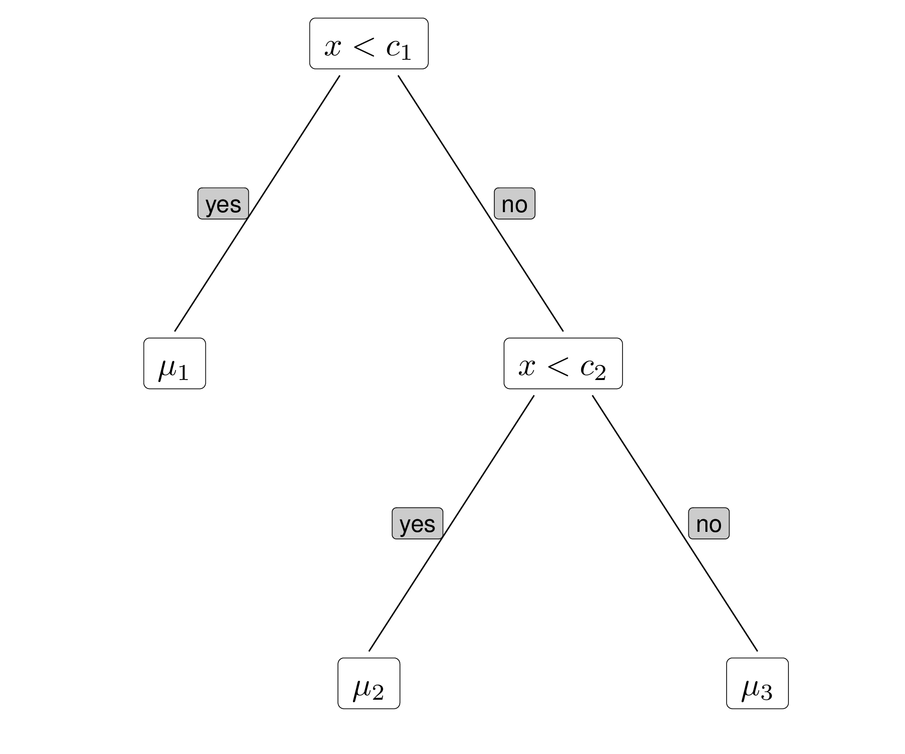
Figure 12.4 shows this process graphically. Figure 12.4 (a) depicts the decision tree for a fictional case in which we only consider a single covariate \(x\) and a decision rule based on cutoffs \(c_1\) and \(c_2\). For each tree that we decide to consider in the process, the parameters \(\mu_1,\mu_2,\mu_3\) are estimated by the data, e.g. using the observed sample mean for the outcome \(y\) in the subset where \(x<c_1\), or where \(x\in (c_1;c_2)\) or where \(x>c_2\), respectively.
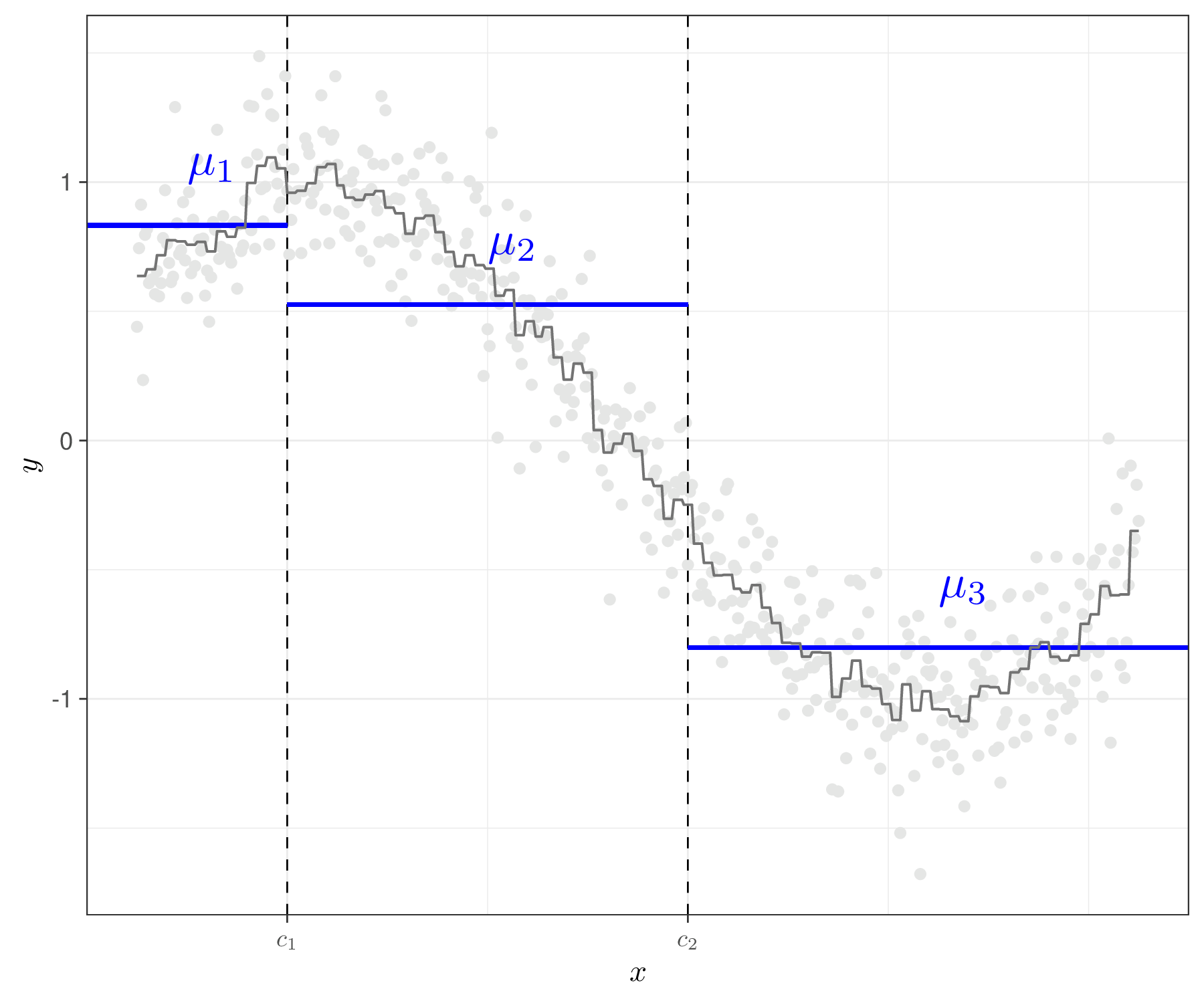
Figure 12.4 (b) shows the estimated configuration for one particular run (i.e. a single tree). As is possible to see, this is a very rough approximation of the underlying relationship between \(x\) and \(y\) – in this case, we are basically fitting a piecewise function to the data. However, if we use a large enough number of trees, then the ensemble combination (which effectively is some kind of weighted average of all the trees) will be flexible enough to estimate the underlying sinusoidal relationship between \(x\) and \(y\) (shown by the grey points).
In order to avoid overfitting for any of the single trees used to approximate the function \(g(\cdot)\), BART uses a naturally Bayesian approach and suitable “regularisation” priors, to ensure that each tree contributes to a limited part of the overall estimation, guaranteeing much flexibility in the resulting estimate. Posterior inference in BARTs can be done using suitable MCMC extensions, usually embedding Metropolis within Gibbs samplers (see Section 2.3).
In line with its machine learning nature, BART is specifically designed for regression models including a large number of predictors and thus it may work particularly well to compute the EVPPI when \(Q_{\boldsymbol\phi}\) is very large, thus overcoming some of the computational limitations of GAMs and GP regression, although this comes at the expenses of the smoothness with which the resulting estimated function is produced. The package voi implements BART as one of the strategies to compute the EVPPI.
12.4.3 Interpreting the EVPPI
Heath et al. (2024) and the voi package website https://chjackson.github.io/voi, as well as the help functions for the package BCEA contain several worked examples on how to compute the EVPPI (note that objects created by BCEA are in the correct format and can thus be passed as input to the voi::evppi() function). We focus here more on the interpretation of the results.
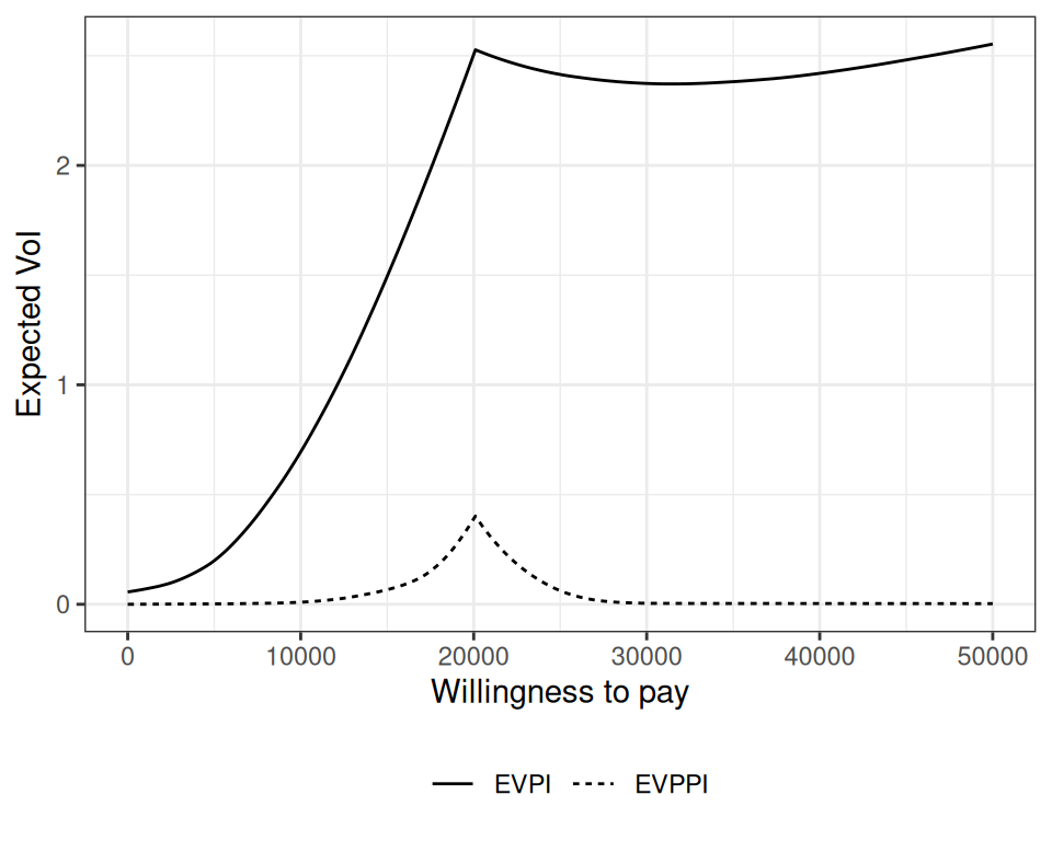
Figure 12.5 shows the analysis of the EVPPI for three of the model parameters1. We can compare the EVPPI (the dashed curve) with the EVPI, computed in Figure 12.2. In fact, the EVPI is the theoretical upper bound for the EVPPI.
In this case, the three parameters contribute relatively marginally to the overall uncertainty – recall that the overall EVPI was perhaps already rather limited (cfr. the discussion in Section 12.3) and thus, given the large number of parameters characterising the model, the combination of this three only determines a fraction of the overall EVPI.
We can also quantify the individual impact of each model parameter in terms of the “single-parameter” EVPPI. BCEA terms this the “Info Rank plot” (Baio et al., 2025), shown in Figure 12.6.
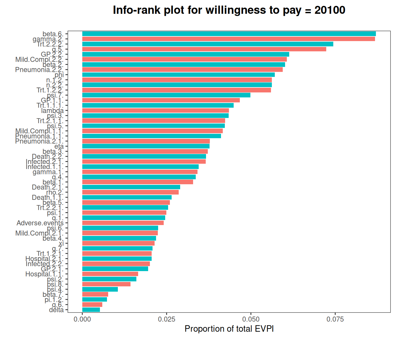
This gives a general indication of the ranking of the various parameters, in terms of their contribution to the overall EVPI and can then be used as a guide to identify which ones are those that should be investigated further. Note however that, as suggested earlier, VoI measures are not additive and thus it is possible that a parameter is associated with a very low single EVPPI, only to interact strongly with another parameter – and thus their joint EVPPI might be very large.
12.5 Expected value of sample information
The final and most helpful measure of VoI is the Expected Value of Sample Information (EVSI). Here, the main idea is to relax the unrealistic assumption of perfect information even further and consider a situation in which we ask ourselves how much it is worth to get some sample information on specific parameters.
The main idea is visualised in Figure 12.7: the top panel is similar to Figure 4.1 and describes the current decision-making process. We collect data (potentially based on a variety of sources, such as literature review, clinical trials and expert opinion), with which we estimate a set of relevant parameters \(\boldsymbol\theta\). These, in turn, inform the economic model, which is used to derive the optimal decision, based on current evidence and our model assumptions (see the discussion in Section 4.2).
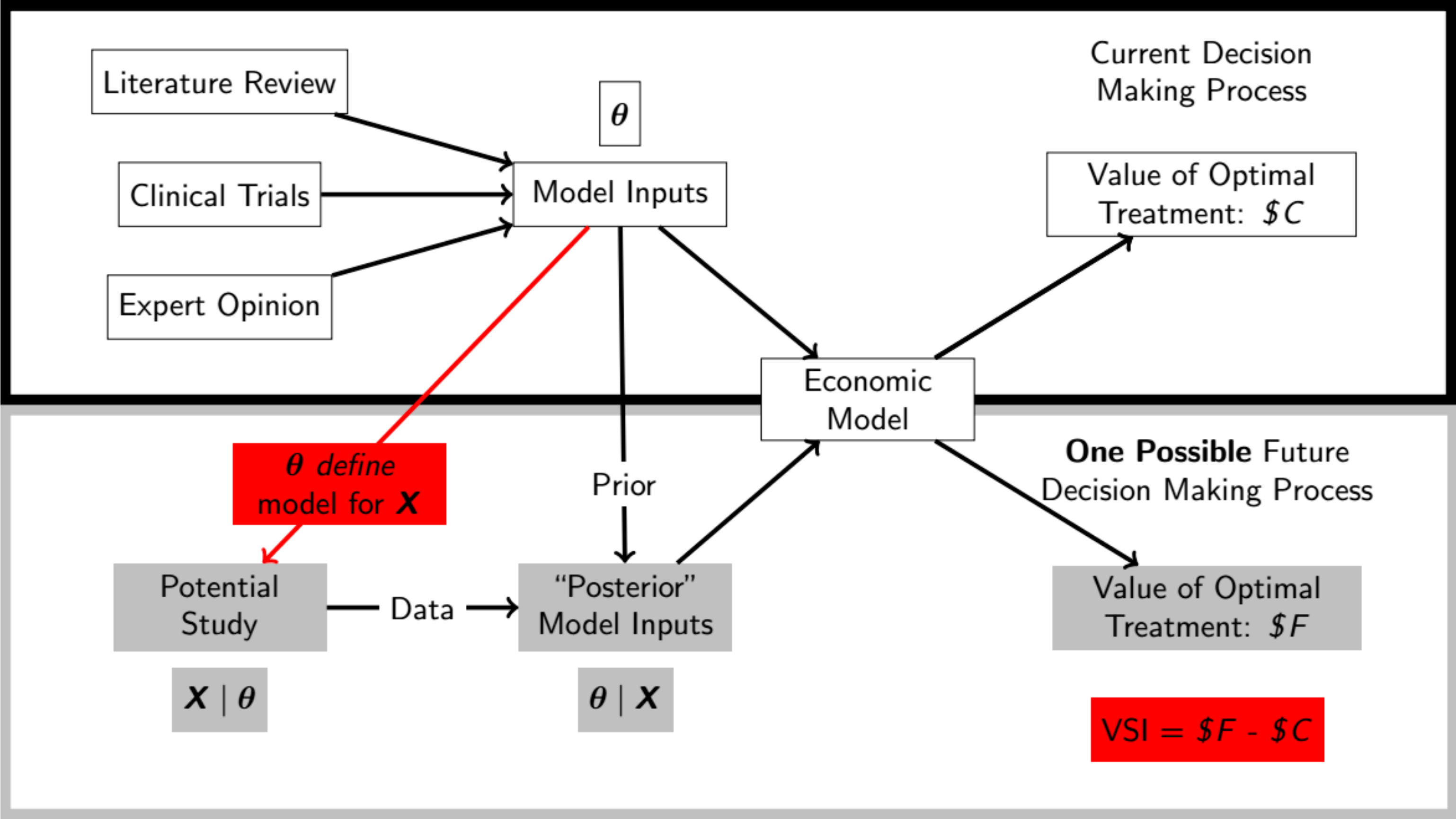
The bottom panel of Figure 12.7 describes the “third option”, i.e. the possibility that, instead of making a decision based on current evidence, we stop and collect new data. The current uncertainty on the model parameters (which is effectively a posterior distribution, based on the observed data) would be used as the prior before observing new data. We can define a sampling mechanism that determines the way in which a potential study would occur and if we actually obtain these new data, then we would update our current uncertainty on \(\boldsymbol\theta\) into a posterior (given the new data \(\boldsymbol{X}\)).
Then we would feed these estimates onto the same economic model and with that obtain a revised decision analysis. The difference between the current value of the optimal treatment (\(\$C\) in the top panel of Figure 12.7) and the revised possible future decision-making process (\(\$F\) in the bottom panel of Figure 12.7) is the value of the sample information that we would have accrued.
Of course, we have not yet obtained the new study and therefore we must include the uncertainty generated by the sampling distribution of the data collection process and average over it to compute \[ \text{EVSI}= \text{E}_{\boldsymbol{X}} \left[ \max_t\ \text{E}_{\boldsymbol\theta \mid \boldsymbol{X}} \left[ \text{NB}_t(\boldsymbol\theta) \right] \right] - \max_{t}\text{E}_{\boldsymbol\theta}\left[\text{NB}_{t}(\boldsymbol\theta)\right], \tag{12.9}\] where \(\text{E}_{\boldsymbol\theta \mid \boldsymbol{X}} \left[ \text{NB}_t(\boldsymbol\theta) \right]\) represents the value of the decision based on sample information \(\boldsymbol{X}\) we may get to see (for a given study design) and, as usual \(\text{E}_{\boldsymbol\theta}\left[\text{NB}_{t}(\boldsymbol\theta)\right]\) is the value of the decision made under current evidence.
In Equation 12.9, because the actual data collection has not happened yet, we must also include an outer expectation with respect to the sampling process \(\text{E}_{\boldsymbol{X}}[\cdot]\) – this adds to the computational complexity to the point that the EVSI was largely just a theoretical concept until the advent of the modern computation techniques described above for the calculation of the EVPPI.
Heath et al. (2024) present detailed accounts of various methods can be used to estimate the value of Equation 12.9, given a specific design and a mechanism to describe the sample variability inherent in the potential collection of data \(\boldsymbol{X}\). These include regression-based tools (effectively the same as in Section 12.4.2), methods that rely on importance sampling (Menzies, 2016) or Gaussian approximation (Jalal et al., 2015; Jalal and Alarid-Escudero, 2018) and moment matching (Heath et al., 2019). The voi package also includes a vignette with worked examples (available at https://cran.r-project.org/web/packages/voi/vignettes/voi.html).
Here, we do not concentrate on the technicalities; instead, we simply highlight the fact that working under an EVSI perspective is just a sensible way of planning future research: not only would we be assessing whether we have enough information in the current evidence in order to make a decision; we would only consider the value-for-money of a potential data collection and thus decide on key features such as design and sample size, in order to maximise the economic value of the new study and subsequent decision-making process.
Example 12.1. Chemotherapy (adapted from Heath et al., 2024). We consider here the Chemotherapy example, originally included in Baio et al. (2025) and then expanded in Heath et al. (2024).
This is based on a Markov model describing the natural history of the disease for a cohort of cancer patients, for whom a specific form of chemotherapy is a viable therapeutic option. The EVSI is the expected value of a two-arm trial with a binary outcome of whether a patient experiences side-effects. The trial is only used to inform the log odds ratio of side effects between treatments and information about the baseline risk of side effects is ignored.
The details of the modelling structure are not too important, here, but they can be found in the voi vignette at https://cran.r-project.org/web/packages/voi/vignettes/plots.html, which also includes R code to generate the analyses and the plots.
Figure 12.8 shows the computed EVSI across a range of potential sample sizes, depending on different values for the underlying willingness-to-pay threshold (in a range from 0 to 50 000 monetary units).
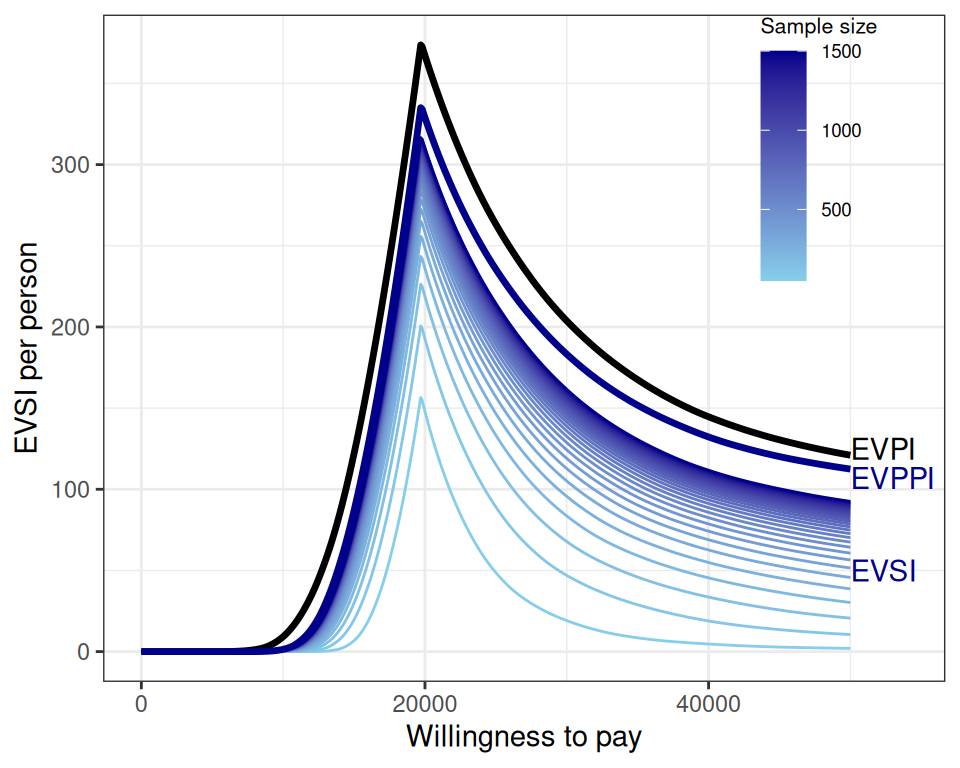
Interestingly, the analysis of Figure 12.8 shows how the EVPI acts as an upper bound to the EVPPI, which in turn acts as an upper bound for the EVSI, when the sample size of the potential data increases sufficiently.
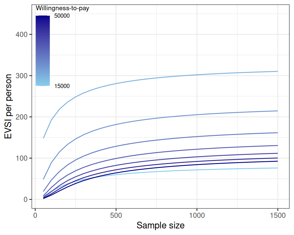
The value of the data collection is marginally decreasing: after a while, there is no point in getting larger and larger sample sizes, as the curves are almost flat at around 1500, along the \(x\)–axis.
12.5.1 Expected net benefit of sampling
We can make better sense of the analysis of the EVSI by considering the actual economic value of a given study in terms of the Expected Net Benefit of Sampling (ENBS). This is defined as \[ \text{ENBS}=\text{EVSI}- \text{expected cost of the study}. \] Here, by “cost of the study” we include the setup cost (e.g. to create the suitable infrastructure needed to deliver an intervention), the cost per individual necessary to buy the intervention (e.g. a given drug), as well as potential other items, including incentives to reduce drop-out. In addition, we typically want to scale this up to the intended target population for whom the technology under investigation will be used and the time horizon that we assume it will be active (e.g. before a new intervention is introduced and replaces the current one as the gold standard).
Of course, these may be complicated to estimate with precision – for instance, we may look into research pipelines to see how many studies are currently being conducted on a given pharmacological indication to get a sense of what the market might look like in the near future. Nevertheless, the ENBS framework forces us to think along those lines, which is helpful to anchor our analysis of the value-for-money of research and the future, potential introduction/reimbursement of a given technology in the real world.
Example 12.2. Chemotherapy (continued): expected net benefit of sampling analysis. Consider first a “standard” sample size calculation that would be performed to design the study. Recall that we are considering here a trial that will investigate the proportion of side effects observed under two interventions. The background probability in the “control” arm (standard of care) is set to \(\theta_1=0.47\), from extensive background knowledge and in order to compute the required sample size, we need to make assumptions on the magnitude of the treatment effect (for the chemotherapy arm).
If we work in terms of OR and assume a substantial reduction in side effects for the chemotherapy, say \[ \text{OR}=\left(\frac{\theta_2}{1-\theta_2}\middle / \frac{\theta_1}{1-\theta_1} \right) = 0.55, \] this also implies that the probability of side effects in the chemotherapy arm is \[ \theta_2=\frac{\theta_1 \text{OR}}{1-\theta_1 + (\theta_1 \text{OR})} \approx 0.37. \]
We can use standard power calculations and the following R code to produce the “power curve” depicted in Figure 12.10.
# Basic assumptions
theta1=0.47
OR=0.55
theta2=(theta1*OR)/(1-theta1+(theta1*OR))

# Standard sample size calculations
ssc=power.prop.test(
  p1=theta1,       # assumed proportion of side effects in the controls
  p2=theta2,       # assumed proportion of side effects in the treatment arm
  sig.level=0.05,  # significance level (to test p1=p2)
  n=seq(0,1500,10) # grid of potential sample sizes
)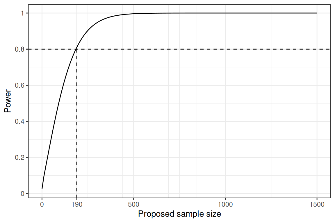
Typically, we select the sample size associated with a value of the power curve of at least some pre-specified threshold, often set at 0.8. In this case, following this rule, the trial would be designed to consider a sample size of \(n=190\) per arm – in Figure 12.10, this is the point along the \(x\)–axis in correspondence of which the power curve intercepts the threshold of 0.8, indicated by the dashed line.
If we perform the analysis based on the ENBS, instead, we obtain the results shown in Figure 12.11. Following the voi vignette, we stipulate that the costs of the study include a fixed setup cost, which we assume ranges between \(5000000\) and \(10000000\) monetary units (say, £), as well as a cost per individual, assumed to range between 14 000 and 21 000 monetary units. We also explicitly consider a target population of around 46 000 patients who would be affected by the change in practice from the standard of care to the chemotherapy and a time horizon of 10 years (over which we apply an annual discount rate of 3.5%) – all the details are described more thoroughly in Heath et al. (2024).
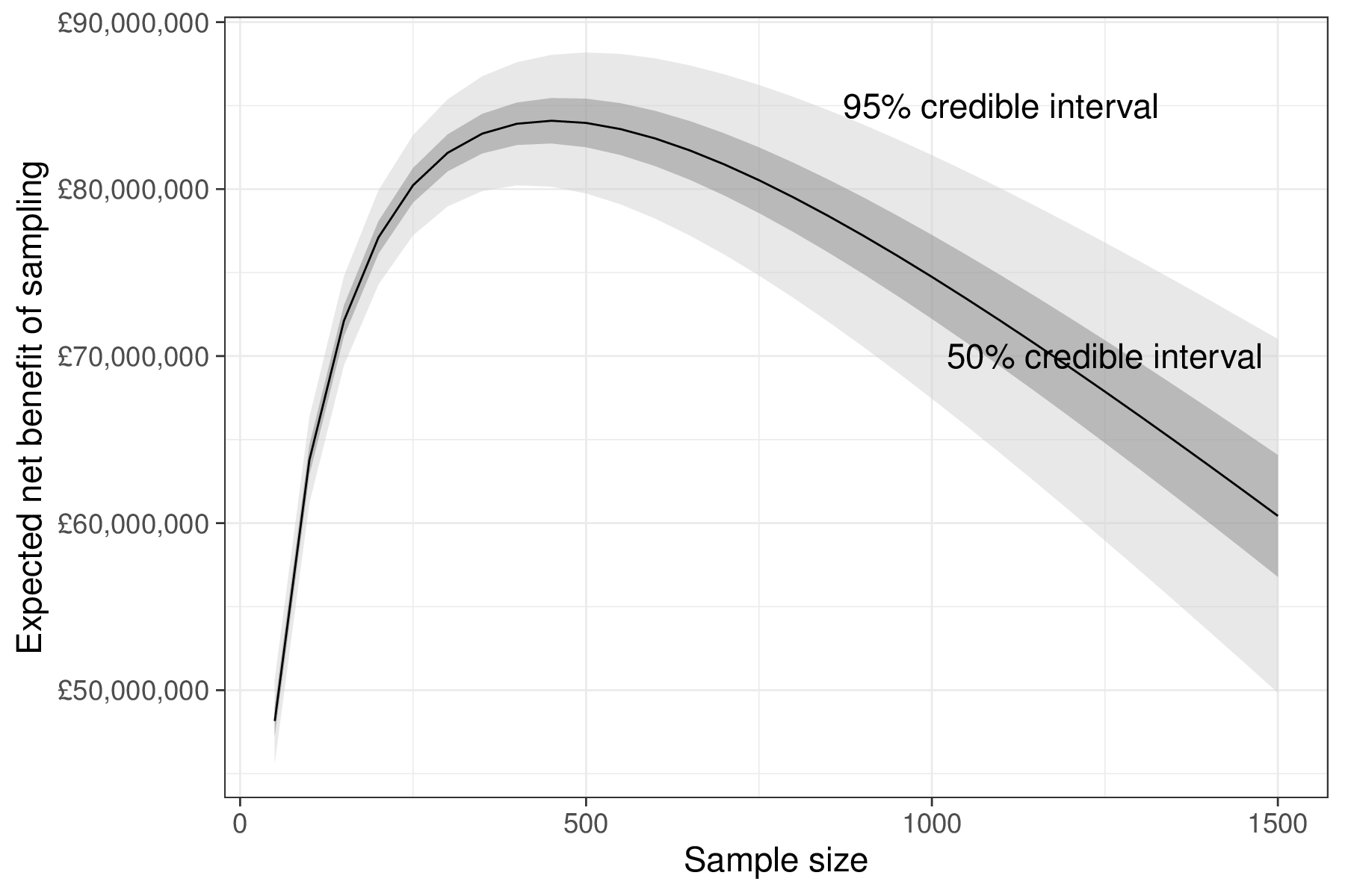
The analysis of Figure 12.11 shows clearly that the “standard” trial would not optimise the economic value of the study: for a sample size of \(n=190\) and assuming a willingness-to-pay threshold for the underlying economic analysis of \(k=20000\) monetary units, the overall ENBS is approximately 77 115 463. This is much lower than the maximum value in the curve of Figure 12.11, which for a sample size of \(n=450\) reaches the maximum value of \(\text{ENBS}=84091443\).
Perhaps, we may not afford to recruit a total of \(450\) patients per arm, in our trial and thus we may need to settle for lower economic value. In any case, the analysis of the ENBS provides a more appropriate assessment of the value for money that we are implying with the specific study design and thus considerations of suitable compromise in terms of the sample size would be made on the relevant monetary scale.
12.6 Conclusions
Although VoI has not been fully included in the normal workflow and processes for HTA, there have been several instances in which regulators have started to open up to this methodology and its application for uncertainty analysis, research prioritisation and planning.
VoI has many important features, particularly within the HTA problem, notably the fact that all the design and analysis is grounded in the full economic evaluation. This has implications even just at the design of the study, because basing it on VoI would force the analyst to construct a model of analysis that closely aligns with it, thus rendering the full evaluation potentially more relevant.