model {
  for (i in 1:N) {
     y[i] ~ dnorm(mu[i], tau)
     mu[i] <- alpha + beta*x[i]
  }
  tau ~ dgamma(0.1,0.1)
  sigma <- pow(tau,-0.5)
}3 Bayesian software
3.1 Introduction
As discussed in Section 2.3, if it is possible to sample from the full conditional distributions, suitable Markov Chain Monte Carlo algorithms (e.g. a Gibbs sampler) can be programmed in a relatively easy way. However, in most practical situations, the required conditional distributions are not analytically tractable and therefore it is necessary to approximate them (e.g. by means of algorithms such as Metropolis-Hastings or slice sampling) before a machinery such as the Gibbs sampling can be put in place.
In this chapter we look specifically at how Bayesian modelling can be performed using specialised software – we concentrate on popular Gibbs sampling programmes (such as the various flavours of BUGS). There are of course other possibilities and the review we provide below is far from exhaustive. On balance, however, for the vast majority of applications in health technology assessment, Gibbs sampling is probably sufficient; in addition, while not necessarily the most frequent tool for inference in this application area (yet…), BUGS-like models are reasonably popular with health economists (particularly in the case of evidence synthesis – see Chapter 6).
For this reason, we concentrate on them both in this chapter and for the vast majority of the rest of this book.
3.1.1 BUGS/JAGS
The most popular software that allows the semi-automation of MCMC procedures is probably BUGS – with this term we indicate the original incarnation (Spiegelhalter et al., 1996)1, the MS Windows version WinBUGS (Spiegelhalter et al., 2002) and its successor OpenBUGS (Lunn et al., 2009; Lunn et al., 2013), whose widespread use has arguably contributed to the establishment of applied Bayesian statistics, in the last thirty years.
The acronym BUGS stands for Bayesian analysis Using Gibbs Sampling and the process requires the user to specify a statistical model (e.g. a set of distributional and functional relationships among the quantities involved in the problem), for example such as the following code (we provide more details on the BUGS syntax in Example 3.1).
The BUGS code always starts with the keyword model, followed by “curly brackets” {} that enclose the model specification. The syntax maps very closely to the standard, “pen-and-paper” statistical notation, with the symbols ~ and <- indicating stochastic and logical relationship, respectively; for instance, the model described above can be written in statistical language as \[\begin{eqnarray*}
y_i & \sim & \text{Normal}(\mu_i,\sigma) \qquad \mbox{for } i=1,\ldots,N \\
\mu_i & = & \alpha+\beta x_i \\
\tau & \sim & \text{Gamma}(0.01,0.01)\\
\sigma & = & \tau^{-0.5}
\end{eqnarray*}\] – note that \(\tau\) is the precision (= inverse variance), which is used in BUGS to index the Normal distribution, alongside the mean.
Note 3.1: Precision vs standard deviation
The fact that BUGS defines the Normal distribution in terms of the precision is pretty much a historical accident. In a Normal model, the precision is useful because it is possible to derive a conjugate prior (see Section 2.2.2 and Example 2.7) and thus when designing BUGS in the early days of the “Gibbs sampling revolution” (see Section 2.3), the coders took advantage of this specific parameterisation, which could be vital in speeding up the computation.
The notation has since stuck and even later versions of BUGS have continued to use this parameterisation. Other Bayesian software (e.g. Stan – see Section 3.1.2) have favoured a more natural parameterisation for a Normal distribution (i.e. in terms of mean and standard deviation), which is sometimes easier to deal with.
BUGS has a built-in parser, which inspects the set of declarations and translates them into a DAG (see Section 1.1), exploiting as much as possible the underlying conditional independence relationships. These generally make the computation simpler and faster, because only a small portion of the whole model needs to be considered at any given time (Lunn et al., 2013).
The DAG resulting from the code above is shown in Figure 3.1, where nodes are represented in ovals; single arrows indicate probabilistic relationships, while double-edged arrows indicate logical relationships, e.g. the node sigma depends logically on the node tau through the relationship sigma <- pow(tau,-0.5), which maps onto the mathematical relationship \(\sigma=\tau^{-0.5}\). The “plate” (i.e. the rectangles) enclosing the nodes y[i], x[i] and mu[i] indicate that their values and underlying relationships hold for (i in 1:N), i.e. for the \(N\) observations.
By and large, BUGS allows models of (almost) arbitrary complexity. The software includes an “expert system”, which determines an appropriate MCMC scheme to be used in the simulation procedure. When possible, BUGS exploits conjugacy (see Section 2.2.2) to speed up the process; when this is not possible, alternative algorithms are used to obtain the required MCMC estimation.
As mentioned above, there are three main versions of BUGS. The first one (called WinBUGS), which can be downloaded at https://www.mrc-bsu.cam.ac.uk/software is an established and stable, stand-alone version of the software. While still available (the latest and last version is 1.4, dating back to August 2007), WinBUGS is not further developed.
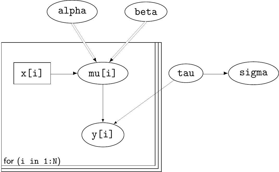
BUGS starting from the linear regression model assumptions passed by the user. Ovals indicate modelled variables, while rectangles indicate observed, but unmodelled data. Single-edged arrows indicate probabilistic dependence, while double-edged arrows indicate logical relationships. The “plates” surrounding the variables indexed by [i] indicate that the structure of relationships and data are for N overall units.
The second (OpenBUGS, also available at https://www.mrc-bsu.cam.ac.uk/software) is an open-source version of the software. At the time of writing this book, the latest release of OpenBUGS is 3.2.2 and it has been designed to be at least as efficient and reliable as WinBUGS over a wide range of test applications.
Finally, the most recent version is called MultiBUGS (Goudie et al., 2020), downloadable from https://www.multibugs.org, which automatically parallelises the MCMC algorithm to speed up computation. The syntax for the three versions of BUGS is essentially identical and the same code should work on either.
Another very relevant and popular “dialect” of the BUGS language is JAGS (Just Another Gibbs Sampler – Plummer, 2010; Kruschke, 2015), which can be downloaded from the website https://mcmc-jags.sourceforge.io. While WinBUGS and OpenBUGS are written in Component Pascal2, JAGS is written in C++, which effectively makes it platform-independent. Because every operating system has a C++ compiler and standard library, JAGS can be run natively under MS Windows, Unix/Linux or Mac. Similar to BUGS, JAGS can be interfaced with R by means of suitable libraries.
For this reason3, JAGS is the preferred tool for Bayesian inference in this book.
3.1.2 Other Bayesian software
Following the introduction of BUGS, much research has also been devoted to developing more software specifically designed for Bayesian analysis. More recently, new MCMC methods have been developed in the form of Hamiltonian (or Hybrid) Monte Carlo (HMC, Duane et al., 1987) – see also Section 2.3.3. Hoffman and Gelman (2013) and Betancourt (2018) have implemented a very clever algorithm that is at the heart of Stan (https://mc-stan.org/), another Bayesian sampler programmed in C++ that can be used very efficiently, particularly for hierarchical models (Gelman et al., 2013). The package rstan interfaces the C++ original code from R, which has contributed to the increasing popularity of this mode of inference. Kruschke (2015) and McElreath (2015) provide extensive examples of implementation of Bayesian models using R and rstan.
Another very interesting development is Integrated Nested Laplace Approximation (INLA, Rue et al., 2009; Blangiardo et al., 2013; Blangiardo and Cameletti, 2015; Wang et al., 2018; Gómez-Rubio, 2020). INLA (implemented in the package R-INLA, downloadable at http://www.r-inla.org/) is a very fast approximate Bayesian inference method; for a relatively wide class of models, INLA can be used to compute the marginal posterior distribution of the parameters without using MCMC, which usually produces a substantial decrease in the computational time. In the context of this book and HTA in general, both Stan and R-INLA can be used in survival modelling (Chapter 8), while Stan is the core engine for Bayesian modelling of indirect treatment comparisons (Chapter 11).
As suggested above, a common characteristic of all these programmes is the possibility to interface each of these with statistical software, e.g. with R. This means that the whole process of Bayesian analysis can be run using R to pre-process the data (e.g. by loading a dataset and creating relative variables), run the Bayesian analysis (e.g. MCMC, HMC or INLA) using BUGS, JAGS, Stan or INLA in the background and then use R to post-process the resulting posterior distribution, for example to assess convergence, plot histograms or compute functions of the parameters. This simplifies and help standardise the whole process of Bayesian analysis.
In a slightly different, but related way, NIMBLE (https://r-nimble.org/, NIMBLE Development Team, 2016) and greta (https://greta-stats.org/) are R packages that can be used to perform MCMC inference directly from R; instead of leaving the simulation from the posterior distributions to a specific software, NIMBLE works by letting the user specify the model in a BUGS-like syntax and then uses C++ to compile and run the required algorithms. greta builds statistical models interactively in R, and then sample from them by different types of MCMC algorithms, including HMC. Finally, Python (https://www.python.org/) and Julia (https://julialang.org/) are very popular with “data scientists” and have specific modules for Bayesian inference.
Pragmatically, what software is used for Bayesian modelling is not really that relevant, provided the user is able to understand the actual modelling specification and what the underlying inferential algorithm is actually doing. As mentioned above, however, we feel that BUGS-like programmes are probably still the most cost-effective for applications in HTA.
3.2 Running JAGS from R
Historically, BUGS was built to run as stand-alone, with a specific graphic user interface. Pretty soon, however, this has been effectively superseded by several packages, macros or add-on that would allow to interface it with “proper” statistical software, such as R, Matlab, Stata or SAS.
The main reason for this is that in essence, BUGS is not a statistical language; rather it is a set of instructions that are used to figure out the most efficient way of producing simulations from a target probability distribution. As such, pre-processing, data wrangling, graphing and reporting facilities are extremely limited in BUGS. Interfacing with statistical software overcomes this limitation – and this has further contributed to the success and wide use of BUGS.
We thus need a suitable library to interface R with the MCMC software of choice. For JAGS, we use R2jags (Su and Yajima, 2010), which is based on rjags (Plummer, 2023), while for BUGS it is possible to use packages such as R2WinBUGS (Sturtz et al., 2005) or R2OpenBUGS (Sturtz et al., 2019). These packages allow the user to perform the analysis from within R by running BUGS/JAGS in the background and they can be installed as usual.
install.packages("R2jags")
install.packages("R2OpenBUGS")
Note that we do not require both BUGS and JAGS (and thus the respective R packages) – we can choose the one we prefer (which may depend on the operating system and/or other considerations) and just have that installed on the machine. Again, in the examples in the next chapters, we will use primarily JAGS.
In general, the process works as follows:
- Use
Rto pre-process the relevant data; this may entail loading a dataset from a spreadsheet or external file, creating new variables, by aggregating or modify existing ones, etc. - Code the statistical model to be run (typically in an external text file) and use suitable commands to launch either
JAGSorBUGSin background. - Once the MCMC run is finished, the simulations become available in the
Rsession where the user is able to post-process them to complete the Bayesian analysis, for instance to produce tables and graphs.
Example 3.1. Drug (continued): conjugate analysis calling JAGS from R. Consider again the situation described in Example 2.3, where we have managed to perform a small pilot study in which we have observed \(y=15\) in \(n=20\) individuals to whom we have given the back-pain relief drug. We can replicate the analysis using JAGS, but we also expand the scenario shown in Example 1.5. In that case, we propagated the uncertainty in the prior distribution and produced MC samples from the prior predictive distribution.
In the current case, we have already gone beyond that stage, because we have observed \(y\) – thus we can update the uncertainty in \(\theta\) to the posterior \(p(\theta\mid y)\) and then use that to propagate the revised level of knowledge and compute, by means of simulations, the posterior predictive distribution \[p(y^*\mid y) = \int p(y^*\mid \theta) p(\theta\mid y) d\theta \tag{3.1}\] (compare this with Equation 1.7).
In other words, we may want to assess what we could reasonably expect if we were able to observe, in the future, a further sample (say of \(m\) new observations): how many \(y^*\) would we reasonably observe, given the current evidence?
We need to map the modelling assumptions in the BUGS language. Fortunately, this is fairly straightforward as most of the syntax is relatively similar to how we would describe the model in “pen and paper”. For the current example, the model code is something like the following.
model {
   theta    ~ dbeta(a,b)                 # prior distribution
   y        ~ dbin(theta,m)              # sampling distribution
   y.pred   ~ dbin(theta,n)              # predictive distribution
   P.crit  <- step(y.pred - ncrit + 0.5) # =1 if y.pred >= ncrit
                                         # =0    otherwise
}
In the code above, y and y.pred share the same distributional assumption.
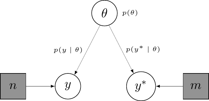
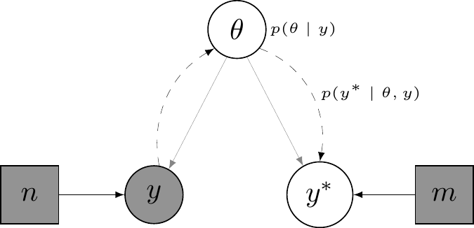
In DAG terms, we could represent this situation as in Figure 3.2: panel (a) shows the alleged data-generating process. The two observable variables \(y\) and \(y^*\) are assumed to be generated by a common mechanism, depending on a parameter \(\theta\), for which we are willing to describe our current uncertainty using a distribution \(p(\theta)\) and suitable observed constants (hence represented in grey squares), \(n\) and \(m\) – technically, \(y\) and \(y^*\) are said to be exchangeable (see Section 6.2.4). Random, yet unobserved, or simply unobservable variables are depicted in white circles.
Panel (b) in Figure 3.2 shows the update process. When data \(y\) are observed (indicated by the fact that the node y is now represented in a grey circle), then the information travels “against the arrows” of the DGP, to update first the uncertainty on the unobservable parameter \(\theta\) into the posterior \(p(\theta\mid y)\). This in turn is used to update the uncertainty in yet unobserved, but potentially observable \(y^*\)
There are several ways to pass the model code to JAGS; the easiest is to save the code above onto a text file, say drug-MCMC.txt. Other alternatives are possible, which may be more efficient, in some cases, when integrating the JAGS analysis into an R script – we return to this in Note 3.2 below.
The second piece of key information that we need to pass onto JAGS is the list of data. We can do so with the following R code.
# Creates the list of data
data=list(
  a = 9.2, b = 13.8, # prior parameters
  y = 15,            # number of successes
  m = 20,            # number of trials
  n = 40,            # future number of trials
  ncrit = 25         # critical value of future successes
)
This is a “list” (we shall see a lot more of this). It is generally a good idea to keep the code general and then pass values that can be changed separately, rather than “hard-coding” them in the model code.
Finally, we can provide a list of “initial values”. In a JAGS/BUGS file, all variables that are associated with a probabilistic statement (i.e. a “~” symbol after the variable name) and are not observed need to be initialised so that BUGS can run the Gibbs sampler. In this particular case, although y is defined as a random variable, because it is also observed, then there is no uncertainty about its value and so we should not initialise it. Conversely, although y.pred has exactly the same nature as y, because it is not observed, then we need to initialise it4. We can either pass specific values for those variables, or leave to JAGS the job of specifying them (more on this later).
Running the model
We are now ready to call JAGS in the background and perform the MCMC analysis
# First load the 'R2jags' package
library(R2jags)

# Then calls the function 'jags' to call 'JAGS' in the background
# and perform the MCMC analysis
model=jags(
  data=data,
  parameters.to.save=c("y.pred","theta","P.crit"),
  inits=NULL,
  model.file="PATH_TO_THE_MODEL_CODE_FILE",
  n.chains=2,
  n.iter=6000,
  n.burnin=1000,
  n.thin=1,
  DIC=TRUE
)
– note that we can run the model using BUGS instead, by simply modifying the command library(R2jags) to library(R2OpenBUGS) and then model=jags(...) to model=bugs(...).
Once the package R2jags is loaded, we can use the function jags(), which takes several inputs – the following are the most important, but others are discussed in later examples and chapters.
data=data: instructsJAGSto look for data in the objectdata(defined as a list, above);parameters.to.save: these are a vector of strings including names of the variables defined in the model code and that we wantJAGSto monitor (i.e. to store values simulated from their relevant distributions);inits: we use this option to specify the initial values from whichJAGSshould start the MCMC process. In this case we set it toNULL, which means thatJAGSwill take care of this steps;model.file: here we specify the path to the (external) file in which we have saved the model code. If the file is not in the current directory, we should specify the full path to it (but see also Note 3.2 below);n.chains: this specifies the number of chains to be run byJAGS(in this case, 2);n.iter: the number of iterations of the Gibbs sampler that we wantJAGSto run;n.burnin: the number of iterations that we wantJAGSto discard. This is typically a very important part of the process as, in general, it may take some time for the Gibbs sampler to converge to the target (posterior) distributions in its exploration of the parametric space. In this particular case, because the underlying model is conjugated (and thus we do not really need to do MCMC), we could even setn.burninto 0, knowing that convergence is immediate. In more general cases, we should ensure that this stage of the process is run for long enough before we can trust the simulations to be drawn from the actual target posterior (see Section 2.3.2);n.thin: the thinning of the chains. It instructsJAGSto only store one everyn.thiniterations (again, see Section 2.3.2 for details). By default,JAGSdoes apply some thinning (see Section 3.3), but here we set it to 1;DIC: if set toTRUE(and in the presence of observed data), instructsJAGSto store the “Deviance Information Criterion”, a measure that can be used to assess model fit (we return to this in Section 5.3.1).
In this case, the model is so simple that this operation is almost immediate and R regains control of the session very quickly.
Post-processing of the model output
The JAGS output is the object model, which can be post-processed using specific functions from R2jags (as well as other packages) – see also Section 3.3 for some more details. For example, we can summarise the simulations using the print() method (here we also use the option digit=3 to specify the number of significant digits to show in the summary table).
print(model,digit=3)Inference for Bugs model at "drug-MCMC.txt",
2 chains, each with 6000 iterations (first 1000 discarded)
n.sims = 10000 iterations saved. Running time = 0.013 secs
mu.vect sd.vect 2.5% 25% 50% 75% 97.5% Rhat n.eff
P.crit 0.327 0.469 0.000 0.000 0.000 1.000 1.000 1.001 10000
theta 0.563 0.075 0.415 0.512 0.564 0.615 0.706 1.001 10000
y.pred 22.511 4.306 14.000 20.000 23.000 25.000 31.000 1.001 10000
deviance 6.640 2.400 3.397 4.828 6.189 7.963 12.463 1.001 10000
For each parameter, n.eff is a crude measure of effective sample size,
and Rhat is the potential scale reduction factor (at convergence, Rhat=1).
DIC info (using the rule: pV = var(deviance)/2)
pV = 2.9 and DIC = 9.5
DIC is an estimate of expected predictive error (lower deviance is better).The summary statistics indicate that, given current evidence, we revise our uncertainty about the true success rate of the drug from a distribution centred on 0.4 and with most of the mass in [0.2; 0.6] to another centred around 0.563 and with most of the probability mass included in [0.415; 0.706]. As for y.pred and P.crit we can see that the expected number of successes in the next phase of the trial is around 23 and the probability of exceeding the critical threshold (25) is 32.68%.
The output model is a very structured object, which contains several other variables and information. These can be accessed and processed, for instance to produce traceplots to assess convergence5 We can use the specialised function traceplot() from the package bmhe, to show the traceplots for selected nodes (among those we have monitored).
bmhe::traceplot(model,"theta")
bmhe::traceplot(model,"y.pred")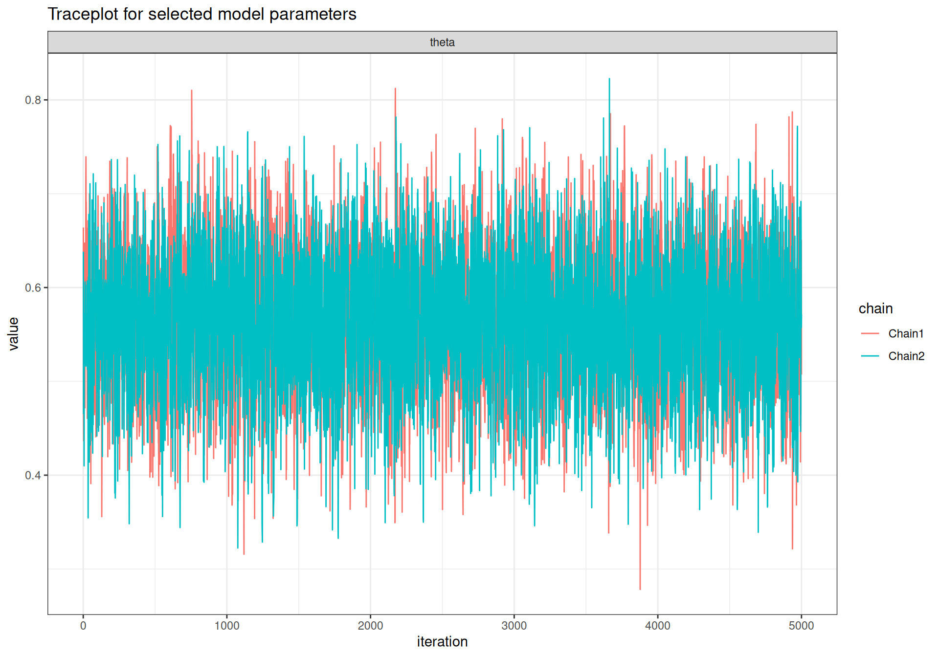
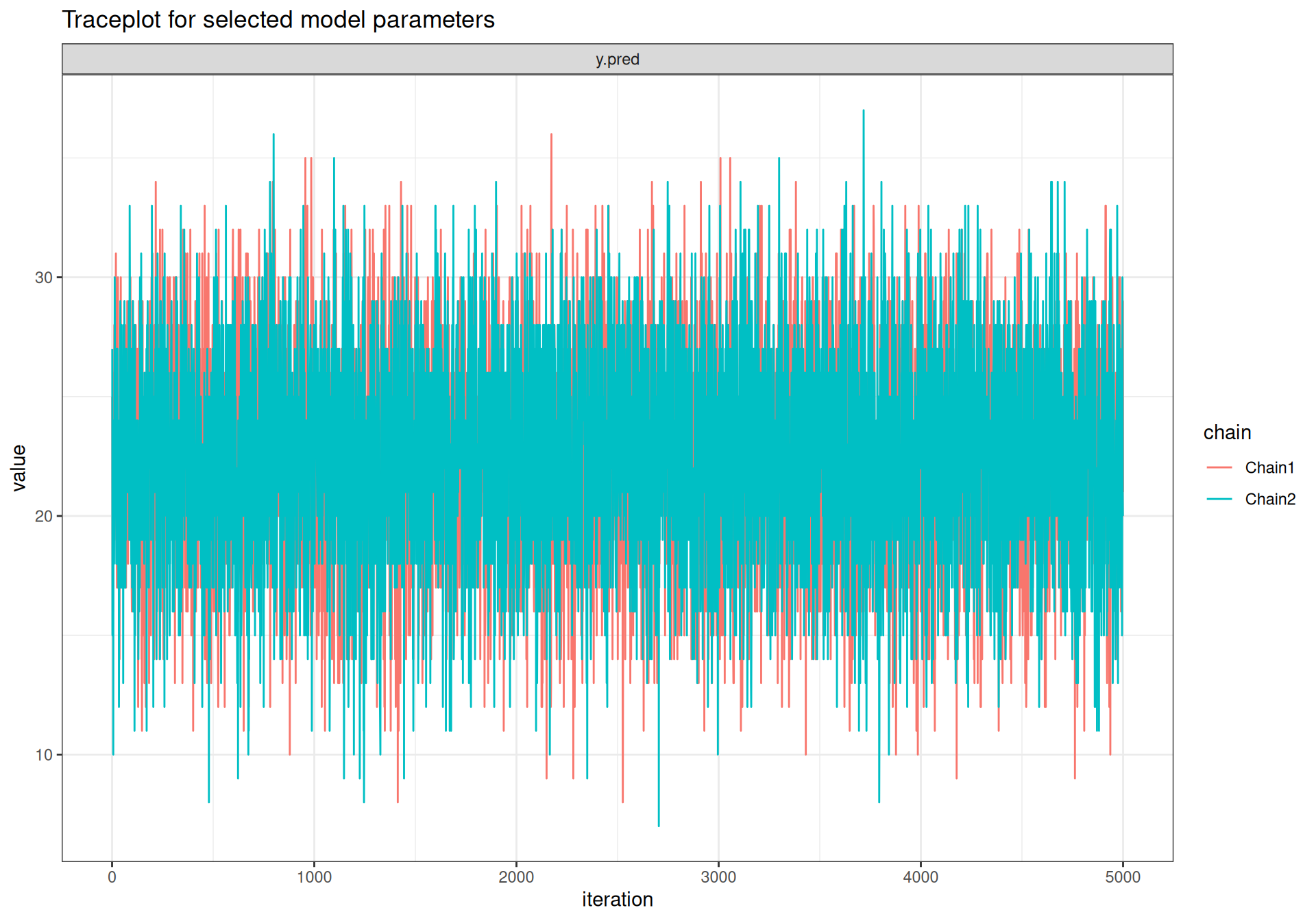
In both cases, already at iteration 1 of the MCMC the two chains that we have run in parallel are on top of each other (we can barely see the lighter lines under the darker ones) and evidently visiting the same portion of the parametric space. This is also confirmed by looking at the more formal convergence statistics: \(\hat{R}\) (Rhat) and the effective sample size \(n_{\text{eff}}\) (n.eff), presented in the last two columns of the summary table shown above (see Section 2.3.2). The former has a value of 1 for all the nodes, well below the rule-of-thumb cutoff of 1.1 – again, given the fact that the model is conjugate, this is not surprising. The model does not present problems in terms of autocorrelation as the effective sample size (giving a measure of how many equivalent independent simulations from the posterior distribution are associated with the possibly dependent vector of MCMC draws) is identical to the nominal sample size (i.e. the number of iterations stored for the MCMC analysis). Figure 3.4 shows the autocorrelation plot for the monitored nodes, using the bmhe function acfplot().
bmhe::acfplot(model,parameter=c("theta","y.pred"),col="red")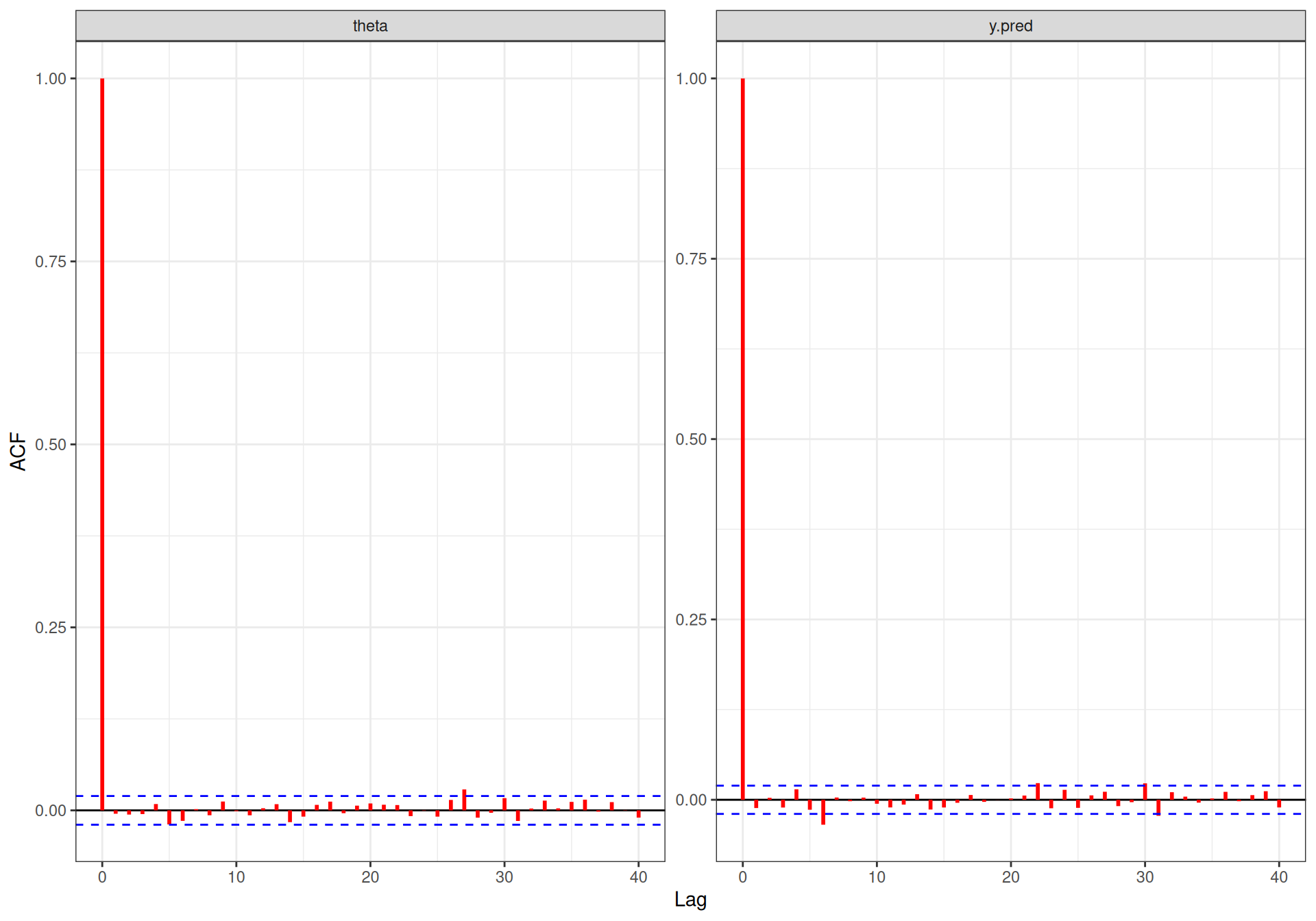
The way in which we need to interpret Figure 3.4 is to look at the level of autocorrelation across different lags. These indicate how much correlation exists across consecutive, lagged simulations in the MCMC procedure. It is expected that consecutive iterations be relatively correlated (because of how the Gibbs sampling is constructed, the \(s-\)th simulated value for the \(q-\)th parameter \(\theta_q^{(s)}\) depends on the distribution at the \((s-1)-\)th run for all the other parameters). But it is also expected that this level of correlation should fade away as we consider simulations that are further apart. So if the autocorrelation graph looks like the ones in Figure 3.4, we can say that actually the simulations are close to a series of independent values because the autocorrelation is very low, in fact at low lags as well.
The formal statistics for convergence (\(\hat{R}\) and \(n_{\text{eff}}\)) can be visualised using the bmhe specialised function diagplot(), as in the following code.
bmhe::diagplot(model,what="Rhat")
bmhe::diagplot(model,what="n.eff")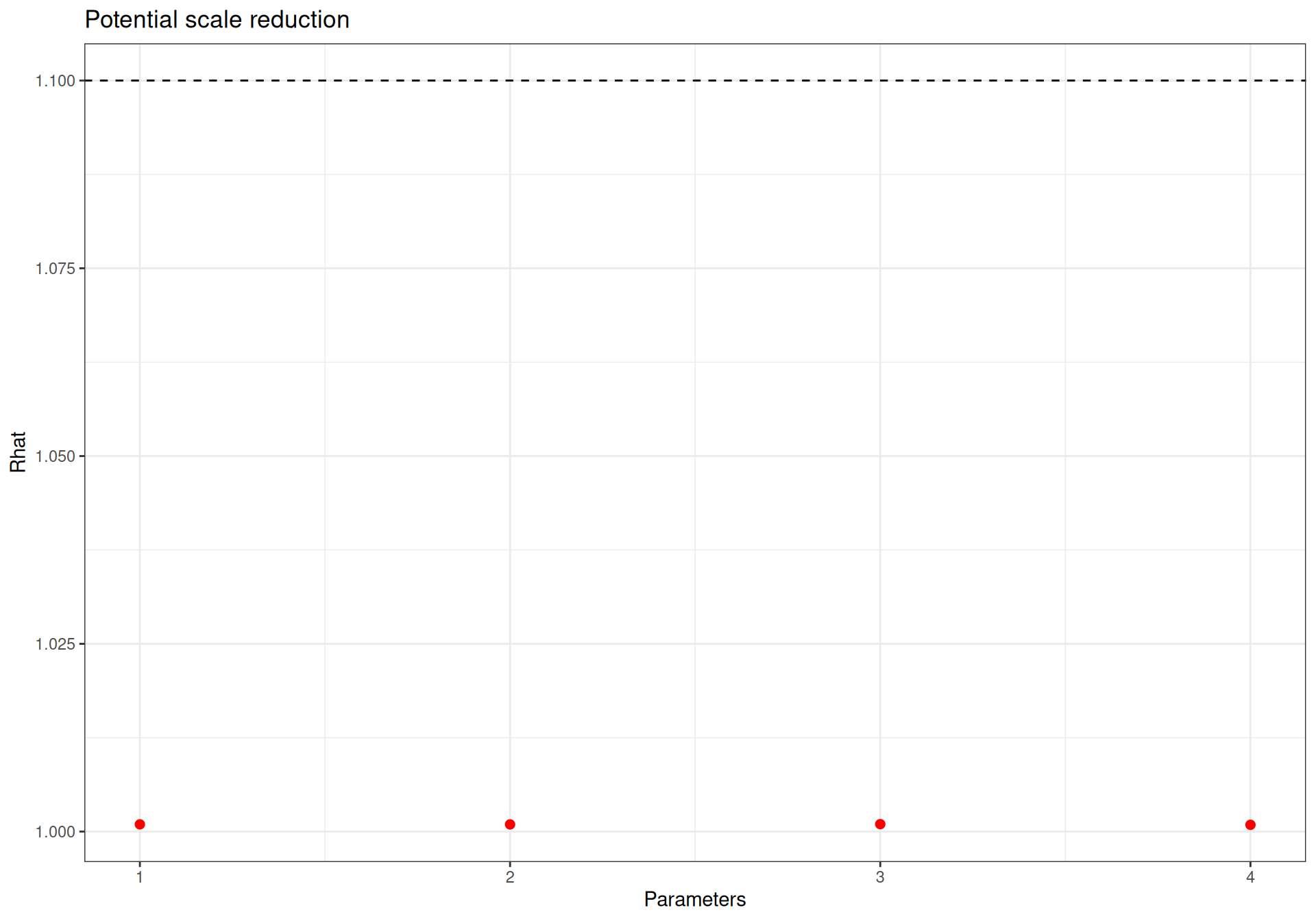
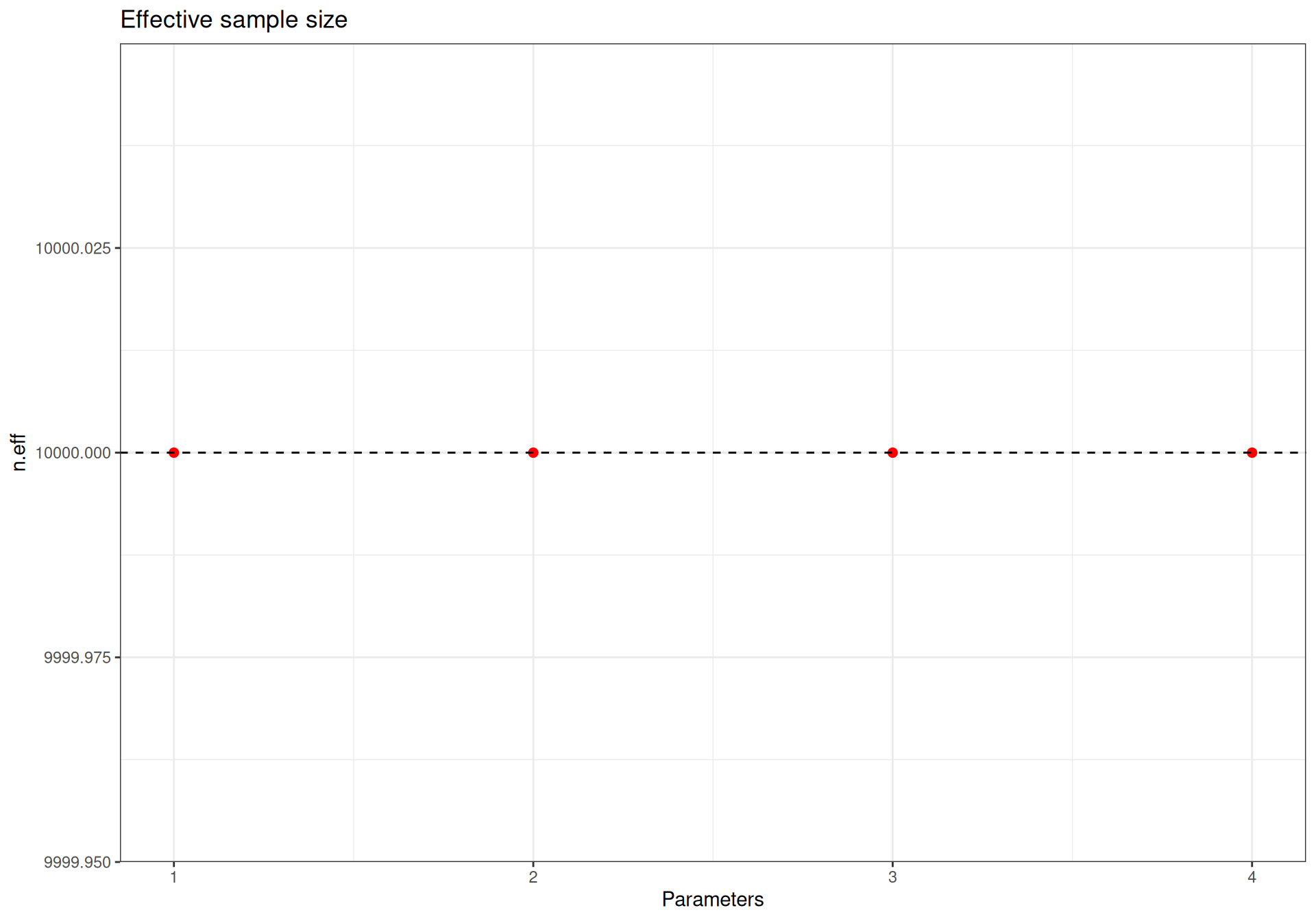
Numerically, when the effective sample size is “close enough” to the nominal sample size (i.e. the number of iterations we use to draw the inference), then autocorrelation is not a problem. In this case, we have considered 2 chains, each with 5000 iterations (so a total of 10 000). The value of n.eff is 10 000 for y.pred, 10 000 for theta and 10 000 for P.crit. The ratios of effective to nominal sample size are then 1, 1 and 1, respectively, which clearly indicate no issues.
We can also use bmhe to visualise the various posterior densities. We choose to do so using the option plot=bar, which shows histograms, but the default plot=density would produce smoothed density estimation for the distributions of interest.
bmhe::posteriorplot(model,plot="bar",parameter="theta")
bmhe::posteriorplot(model,plot="bar",parameter="y.pred")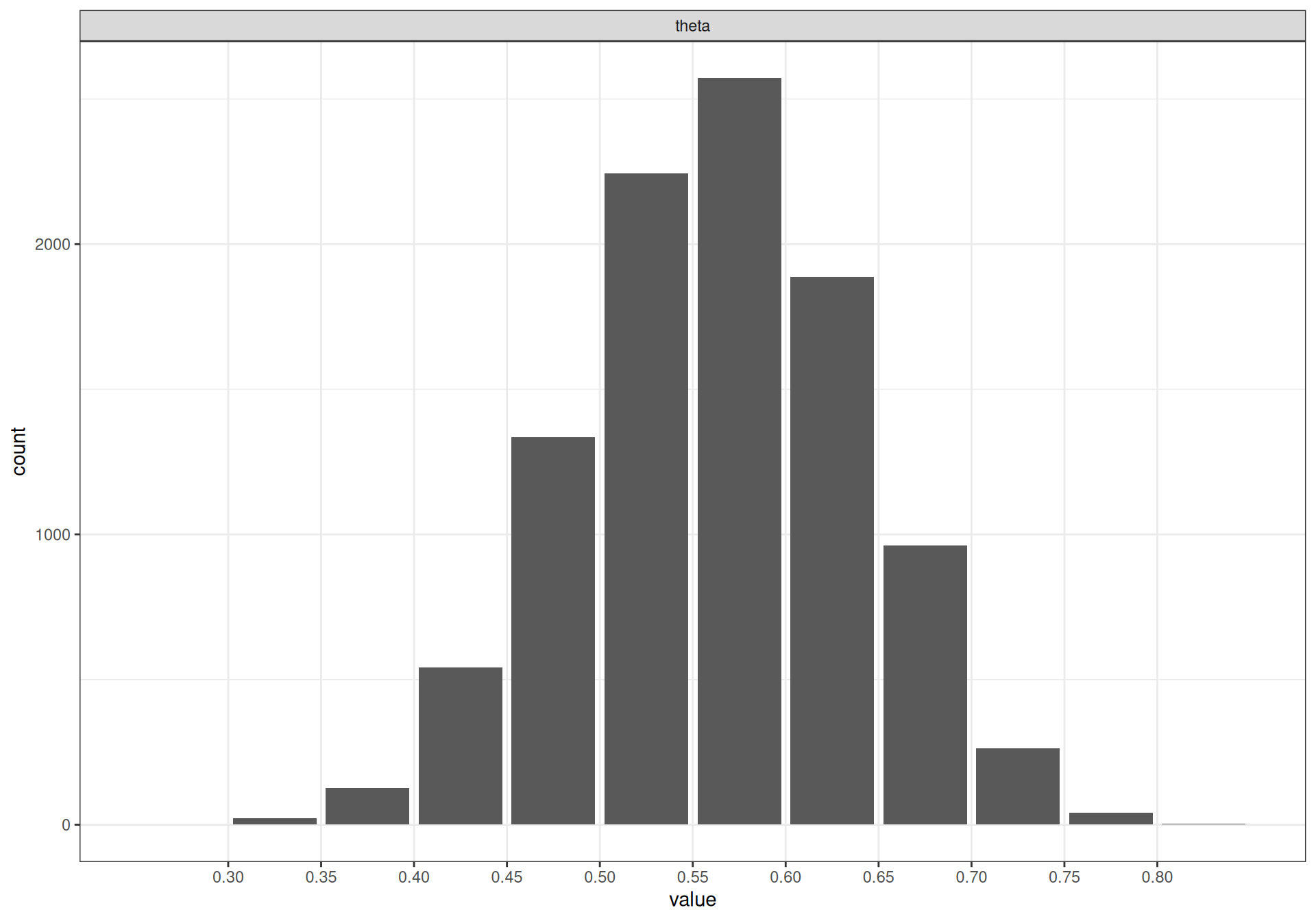
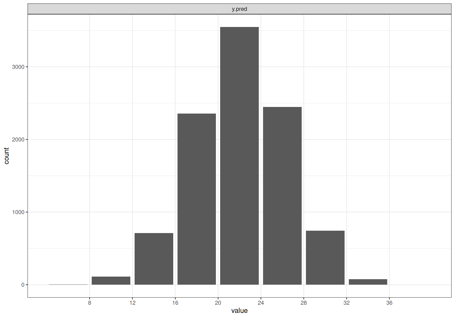
Note that while the graphs look very similar for (the posterior of) theta and (the predictive distribution for) y.pred, the nature of the variables is fundamentally different (cfr. Example 2.1). The former is about the model parameter \(\theta\), which represents a probability and it is thus constrained in the range [0-1], Conversely, \(y_{pred}\) represents the number of successes out of a sample size \(n=40\) and is thus a very different quantity – and in addition, \(\theta\) is continuous and \(y_{pred}\) is discrete!
3.3 Differences between BUGS and JAGS
While a piece of code written in BUGS has almost 100% compatibility with JAGS, there are still some built-in differences between the two; more importantly there are some key distinctions between the R packages used to run the MCMC models, R2OpenBUGS and R2jags.
If we look at the R help for the two main functions6 R2OpenBUGS::bugs() and R2jags::jags(), we can see that quite a few of the default values are not actually aligned, which explains why we may get different numbers when running one or the other – that is with a vanilla version, that does not control for all the underlying options.
# Default inputs for the `R2OpenBUGS::bugs()` function
R2OpenBUGS::bugs(
  data, inits, parameters.to.save, n.iter, model.file="model.txt",
  n.chains=3, n.burnin=floor(n.iter / 2), n.thin=1, saveExec=FALSE,
  restart=FALSE, debug=FALSE, DIC=TRUE, digits=5, codaPkg=FALSE,
  OpenBUGS.pgm=NULL, working.directory=NULL, clearWD=FALSE, useWINE=FALSE,
  WINE=NULL, newWINE=TRUE, WINEPATH=NULL, bugs.seed=1, summary.only=FALSE,
  save.history=(.Platform$OS.type == "windows" | useWINE==TRUE),
  over.relax = FALSE
)

# Default inputs for the `R2jags::jags()` function
R2jags::jags(
  data, inits, parameters.to.save, model.file="model.bug", n.chains=3,
  n.iter=2000, n.burnin=floor(n.iter/2),
  n.thin=max(1, floor((n.iter - n.burnin) / 1000)), DIC=TRUE,
  working.directory=NULL, jags.seed = 123, refresh = n.iter/50,
  progress.bar = "text", digits=5,
  RNGname = c(
    "Wichmann-Hill", "Marsaglia-Multicarry", "Super-Duper", "Mersenne-Twister"
  ), jags.module = c("glm","dic"), quiet = FALSE
)
More specifically, let us see what happens when we actually run them both on the same data without thinking too much. We do this using the “eight schools” example presented in the R help for both R2OpenBUGS::bugs() and R2jags::jags() and originally discussed in Sturtz et al. (2005).
# An example model file is given in:
model.file=system.file(
  package="R2OpenBUGS", "model", "schools.txt"
)
# Can visualise the model uncommenting the following command
# file.show(model.file)

# Some example data (see ?schools for details):
data(schools)

# Makes relevant variables
J=nrow(schools)
y=schools$estimate
sigma.y=schools$sd

# Puts the data in a list
data=list ("J", "y", "sigma.y")

# Functions to generate initial values
inits=function(){
    list(theta=rnorm(J, 0, 100),
         mu.theta=rnorm(1, 0, 100),
         sigma.theta=runif(1, 0, 100)
    )
}

# Defines the model parameters
parameters=c("theta", "mu.theta", "sigma.theta")

# Runs the model using a vanilla BUGS
mbugs=bugs(
  data, inits, parameters, model.file,n.chains=3, n.iter=5000
)

# Runs the model using a vanilla JAGS
mjags=jags(
  data, inits, parameters, model.file,n.chains=3, n.iter=5000
)
The first slightly annoying quirk is that if we inspect the two objects mbugs and mjags we can see that they have a different structure.
names(mbugs) [1] "n.chains" "n.iter" "n.burnin" "n.thin"
[5] "n.keep" "n.sims" "sims.array" "sims.list"
[9] "sims.matrix" "summary" "mean" "sd"
[13] "median" "root.short" "long.short" "dimension.short"
[17] "indexes.short" "last.values" "isDIC" "DICbyR"
[21] "pD" "DIC" "model.file" names(mjags)[1] "model" "BUGSoutput" "parameters.to.save" "model.file"
[5] "n.iter" "DIC" R2jags is perhaps more organised and creates a nested object BUGSoutput, in which it stores all the, well… BUGS output. R2OpenBUGS, on the other hand, stores all the main output directly in the object (in this case, named mbugs). We can use the $ notation to access the elements of the nested object mjags$BUGSoutput; thus, for instance, we can visualise the first few simulated values using the following R code
mjags$BUGSoutput$sims.matrix |> head() |> round(4) deviance mu.theta sigma.theta theta[1] theta[2] theta[3] theta[4] theta[5]
[1,] 63.1957 3.4785 14.2200 26.2666 -16.7075 -9.2396 11.9437 2.4603
[2,] 60.1780 5.0820 2.8610 0.4945 6.6275 1.4543 6.6836 4.9866
[3,] 59.1257 11.6818 9.6859 19.9707 3.7033 -1.6391 5.4203 17.2153
[4,] 59.6005 7.7004 0.6455 8.1408 7.0607 7.2135 5.8920 7.8793
[5,] 57.7529 3.8825 9.1391 12.7300 8.0826 4.1697 -0.7808 8.4334
[6,] 60.2013 4.8843 0.6047 4.7616 5.5125 6.1149 4.9416 5.3324
theta[6] theta[7] theta[8]
[1,] 3.8333 11.0219 -8.8492
[2,] 6.4765 8.2986 4.2943
[3,] -0.3253 17.0090 6.8228
[4,] 8.1308 6.8901 7.4641
[5,] -1.1303 14.1492 12.4989
[6,] 5.3788 4.5440 5.2419while we could simply write mbugs$sims.matrix |> head() if we were post-processing a R2OpenBUGS object. All in all, we can get access to the same information from both packages – it is just in different places and we need to know where to look. Note that the package bmhe, which we use throughout this book somehow mitigates this by using specialised functions that do know where to look and pick up the relevant information, whether the object to be processed is obtained through R2jags or R2OpenBUGS.
Another important difference is perhaps even more subtle. In both cases, we are using n.iter= 5000 (that is the number of total iterations per chain) with n.chains=3 (the default number of parallel chains). In both cases, by default (i.e. unless we say something explicitly different), n.burnin=n.iter/2 and so we have a total of (n.iter-n.burnin) \(\times\) n.chains= (5000 \(-\) 2500) \(\times\) 3 = 7500 iterations. That is the length of the MCMC process.
However, by default, BUGS assumes n.thin=1 (see Section 2.3.2.4), which means that it retains all the 7500 iterations for the MCMC analysis (that is actually stored in the variable n.sims), as we can see from the table below.
print(mbugs,digits=3)Inference for Bugs model at "schools.txt",
Current: 3 chains, each with 5000 iterations (first 2500 discarded)
Cumulative: n.sims = 7500 iterations saved
mean sd 2.5% 25% 50% 75% 97.5% Rhat n.eff
theta[1] 11.185 8.892 -2.787 5.500 9.806 15.663 32.897 1.006 400
theta[2] 7.481 6.504 -4.901 3.363 7.368 11.480 20.810 1.006 380
theta[3] 5.800 8.013 -12.037 1.330 6.370 10.520 20.950 1.003 1000
theta[4] 7.106 6.741 -6.251 3.049 7.133 11.182 20.980 1.005 580
theta[5] 4.908 6.339 -8.841 0.958 5.510 9.134 16.380 1.004 620
theta[6] 5.798 6.787 -9.097 1.754 6.126 10.120 18.356 1.005 490
theta[7] 10.376 7.224 -2.110 5.615 9.710 14.582 26.280 1.008 280
theta[8] 8.092 8.010 -7.132 3.365 7.770 12.440 25.675 1.006 390
mu.theta 7.619 5.439 -2.693 4.123 7.606 11.000 18.630 1.008 290
sigma.theta 6.681 5.877 0.241 2.273 5.283 9.403 21.862 1.004 560
deviance 60.533 2.279 57.005 59.170 60.060 61.560 66.230 1.002 1700
For each parameter, n.eff is a crude measure of effective sample size,
and Rhat is the potential scale reduction factor (at convergence, Rhat=1).
DIC info (using the rule, pD = Dbar-Dhat)
pD = 2.879 and DIC = 63.410
DIC is an estimate of expected predictive error (lower deviance is better).Conversely, JAGS uses by default n.thin=max(1, floor((n.iter - n.burnin)/1000)), which in this case is max(1, floor((5000 - 2500)/1000)) = 2. In other words, of the 7500 iterations that are considered, JAGS retains only one every 2, which means the overall value for n.sims is actually half as that produced, by default by BUGS7.
print(mjags,digits=3)Inference for Bugs model at "schools.txt",
3 chains, each with 5000 iterations (first 2500 discarded), n.thin = 2
n.sims = 3750 iterations saved. Running time = 0.027 secs
mu.vect sd.vect 2.5% 25% 50% 75% 97.5% Rhat n.eff
mu.theta 7.846 5.106 -1.758 4.758 7.725 10.804 18.247 1.002 3800
sigma.theta 6.975 5.524 0.131 2.908 5.892 9.674 20.873 1.022 230
theta[1] 11.808 8.956 -1.977 6.059 10.181 15.909 34.503 1.001 3800
theta[2] 7.638 6.423 -5.300 3.704 7.419 11.387 21.196 1.001 3800
theta[3] 5.950 7.855 -11.879 1.667 6.330 10.431 21.241 1.004 2500
theta[4] 7.453 6.659 -6.156 3.381 7.186 11.428 21.263 1.001 3800
theta[5] 5.109 6.251 -8.358 1.493 5.626 9.063 16.594 1.004 1000
theta[6] 5.800 7.036 -9.660 1.704 6.174 9.900 19.810 1.005 670
theta[7] 10.750 7.083 -1.275 6.084 9.928 14.827 26.562 1.003 3500
theta[8] 8.488 7.870 -6.659 3.751 8.100 12.784 25.586 1.001 3800
deviance 60.378 2.266 56.851 59.039 59.930 61.456 65.924 1.008 780
For each parameter, n.eff is a crude measure of effective sample size,
and Rhat is the potential scale reduction factor (at convergence, Rhat=1).
DIC info (using the rule: pV = var(deviance)/2)
pV = 2.6 and DIC = 62.9
DIC is an estimate of expected predictive error (lower deviance is better).As a result, the efficiency of the two processes is also different – in the case above, note the values of \(n_{\text{\textit{eff}}}\), which are generally higher (with a smaller nominal sample size) for JAGS than they are for BUGS, again due to the impact of thinning, which reduces the autocorrelation in the former in comparison to the latter.
NoteEffective vs nominal sample size and autocorrelation
The summary table for the JAGS model indicates that for some nodes the effective sample size (n.eff) is even bigger than the nominal MC sample size (n.sims), for instance for the node mu.theta. This apparent quirk is due to the fact that \(n_{\text{\textit{eff}}}\) is a function of the underlying autocorrelation in the simulations (see Equation 2.13). When this autocorrelation is negative, the effective sample size gets artificially inflated to values larger than the theoretical upper bound, indicated by the MC sample size. This artefact is also common to Stan, which can return \(n_{\text{\textit{eff}}}>n_{\text{\textit{sims}}}\) for parameters whose posterior is close to a Normal and have little dependency on other parameters (Stan development team, 2024).
More specifically, this means that what is an apparently identical process may in fact be much slower in BUGS, simply because of how it handles the thinning. In BUGS, if we specify n.iter=10 000 and n.thin=20, then BUGS will run the MCMC process for 10 000 \(\times\) 20 = 200 000 iterations so that it can in fact retain one every 20 – that is 10 000 overall. In JAGS, conversely, this would be handled by running the actual number of iterations requested (n.iter=10 000); then, because of the thinning, only 1 in 20 will be retained and so we would end up with only 10 000/20=500 iterations saved.
When initial values are not specified by the user, the two programmes also have slightly different ways of generating them. BUGS generates initial values by forward sampling from the prior distribution for each parameter. Thus, when using very vague priors, it is possible that, by random chance, one of the chains for a given parameter is initialised from a point that is very far from the target area of the posterior distribution, which may slow down convergence. JAGS on the other hand sets all initial values from the “middle” (either the mean or the mode, depending on the distribution) of the prior. On occasions, this may be a safer approach – but ultimately, it is always helpful to at least try a model run with user-specified initial values.
Finally, another important distinction is in the default random seed8: BUGS sets its seed to 1, while JAGS sets its to 123. Generally speaking, none of these differences matter greatly, once the model has converged and run for long enough. A larger n.sims would generally imply a smaller MC error and more precision (and, crucially, a better characterisation of the whole posterior distribution – not just the mean and central part). Even in the case above, for most parameters, the individual statistics are fairly aligned and using one set of estimates instead of the others does not make a huge difference…
3.4 Defining non-standard distributions in BUGS/JAGS
Both BUGS and JAGS have a number of built-in distributions, which cover a vast number of applied cases. There are however circumstances in which we may need to use a formulation that is not available, either for the sampling or the prior distribution.
For example, imagine that we want to model a variable \(y\sim p(y\mid\theta)\), where \(p(y\mid\theta)\) is the required non-standard distribution, indexed by a parameter \(\theta\). The main idea is to use the “zero-trick” (Lunn et al., 2013, sect. 9.5), i.e. to create some fake observation, \(w=0\), which is modelled as \(w\sim\text{Poisson}(\phi)\).
Because we “pretend” that \(w\) is observed to be 0, then its contribution to the overall likelihood is \(\exp(-\phi)\), as is possible to see from Equation 1.1. If we set \(\phi=-\log\mathcal{L}(\theta\mid w,y)\) and model \(y\) using a very flat, non-informative prior, then we retrieve the correct overall contribution to the likelihood and effectively model \(p(y\mid \theta) \propto \exp(-\phi) = \mathcal{L}(\theta\mid w,y)\) – cfr. the discussion in Section 2.2.1.
Notice that we may or may not observe \(y\) (which, in fact, may have the role of a model parameter, when we are trying to define a non-standard prior and thus may not be at all observable, as we show in Example 3.2); if we have no observation on \(y\), we can still construct a likelihood based on the “observation” of \(w\).
Example 3.2. Zero-trick to code a PC prior for Binomial parameter. The PC prior in Equation 2.10 has a highly non-standard format and thus it is not implemented as a built-in distribution to directly use in BUGS/JAGS code. However, if we give \(\theta\) a \(\text{Beta}(1,1)\) prior (which effectively does not contribute anything to the posterior – see again Section 2.2.1) and set \(\phi=-\log \mathcal{L}(\theta\mid w)=-\log p(\theta)\), where \(p(\theta)\) is defined in Equation 2.10, then we will imply the correct likelihood contribution and therefore we will have effectively modelled \(\theta \sim \text{PC prior}(\lambda,\theta_0)\).
We can do so in the JAGS code below.
model_pc_bern=function(){
  # "Pseudo-observation", w=0
  w ~ dpois(phi)

  # Defines the likelihood from the PC prior
  d <- pow(
    2*theta*log(theta/theta0)+2*(1-theta)*log((1-theta)/(1-theta0)), 0.5
  )
  deriv <- abs((log(theta)-log(1-theta)-log(theta0)+log(1-theta0))/d)
  # Models phi as a function of the likelihood for theta
  phi <- -log(lambda*exp(-lambda*d)*deriv) + C

  # "Non-informative" prior for theta, to combine with the likelihood
  # contribution from phi and effectively imply that theta ~ PC prior
  theta ~ dbeta(1,1)
  # Possible data - if not observed, sampling from the prior only
  y ~ dbin(theta,10)
}

# Runs the model in JAGS with no data for y to check what the prior looks like
test=R2jags::jags(
  data=list(y=NA,w=0,C=10000,lambda=1,theta0=0.5),parameters.to.save=c("theta"),
  model.file=model_pc_bern,n.chains=2,n.thin=4,n.iter=100000,DIC=FALSE,
  inits=list(list(theta=0.1), list(theta=0.9))
)
Notice that here we add a large constant \(C=10000\) to the expression for \(\phi\), to ensure that it is positive (as is required, since \(\phi\) is the mean of a Poisson distribution and hence constrained in \(\mathbb{R}^+\)) – this is just a scaling factor.
The results can be summarised by using the print() method. In this case, convergence is reached satisfactorily although, in general, the “zero-trick” method can be prone to poor mixing of the chains.
# Summary results
print(test,digits=3)
Inference for Bugs model at "/tmp/Rtmpm33PHr/modelff5d77b03746d.txt",
2 chains, each with 100000 iterations (first 50000 discarded), n.thin = 4
n.sims = 25000 iterations saved. Running time = 0.143 secs
mu.vect sd.vect 2.5% 25% 50% 75% 97.5% Rhat n.eff
theta 0.503 0.27 0.026 0.293 0.502 0.715 0.976 1.001 25000
For each parameter, n.eff is a crude measure of effective sample size,
and Rhat is the potential scale reduction factor (at convergence, Rhat=1).# MC estimate for Pr(theta>0.75)
sum(test$BUGSoutput$sims.list$theta>0.75)/test$BUGSoutput$n.sims[1] 0.21656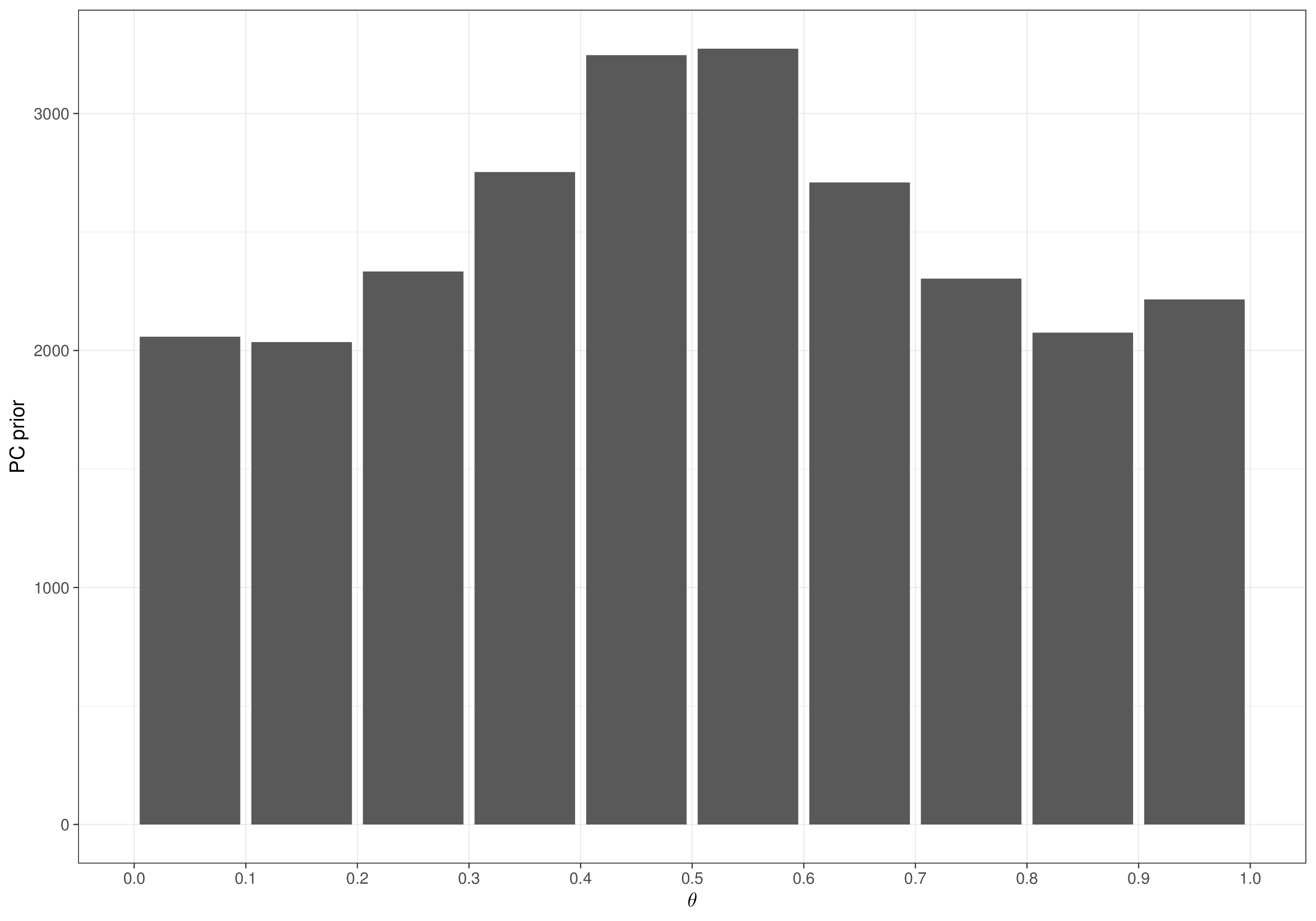
We can see that the empirical estimate or \(\Pr(\theta>0.75)\) agrees with the numerical integration we performed in Example 2.6 (\(\approx 0.22\)) and the resulting prior distribution depicted in Figure 3.7 is also similar to the analytic form presented in Figure 2.10.
In the vast majority of applications of Bayesian modelling to HTA, the practitioner would not be required to define their own specific probability distribution (either to model sampling variability for observable data \(y\) or epistemic uncertainty for parameters \(\theta\)). If that becomes a necessity, perhaps more “modern” software (usually classified as “probabilistic languages”), e.g. Stan or Nimble may be more appropriate and efficient.
For instance, in Stan there is no need to use the zero-trick to adjust the likelihood; instead, it is possible to define a customised distribution in a functions block (see Section 8.3.5 for a specific example and more details on coding Stan models). This would generally work in a more efficient and generalisable way.
3.5 Conclusions
This chapter has given a brief introduction to all-purpose Bayesian software, presenting a list of the most popular and focusing specifically on JAGS and BUGS. These are both based on Gibbs sampling and have already been used relatively extensively in the Health Technology Literature and thus we have selected them (and specifically JAGS) as the main alternative, for the purpose of modelling discussed in this book.
We have given a general introduction to the main setup (which is fairly common for both JAGS and BUGS) and have looked at how it is possible to interface the Bayesian software with R, the language of choice for statistical modelling – other are of course possible (including ones that are very popular in fields such as Data Science, e.g. Python). We have also discussed the general workflow of Bayesian analysis based on running a model in JAGS.
In the next chapter, we will concentrate on a general introduction to the field of Health Technology Assessment (HTA), particularly from a Bayesian perspective. We will present the basic decision problem and the various metrics used to perform the economic evaluation of healthcare interventions and then prepare the setting for later chapters, in which we will go over various statistical modelling specifically for HTA.
The author is nerdly proud of sharing his birthday (only several years earlier…) with the day of the first ever public release of “classic
BUGS”, back in August 1996.↩︎This is a relatively obscure language implemented in a particularly low-level environment, known as Black Box Component Builder, with compiler available only for
MS Windows(although the latest release ofOpenBUGSdoes run underLinuxand, using a virtual machine, underMactoo).↩︎Upon joining UCL in 2005, the then IT manager told me: “I’ll install Linux on your machine. You will probably hate it for a while, but then you will never look back”. I have not looked back.↩︎
In fact, we may get away with not initialising
y.predtoo, because it is a deterministic function of other random nodes (theta, in this case) and thus, by initialisingtheta, we provide enough information forJAGSto initialisey.predtoo.↩︎Again, in this case we do not have to worry about this because of conjugacy (see Section 2.2.2), but we use this example to make the point.↩︎
To highlight that the functions come from different packages, we use the
pkg::func()notation – see the discussion in Note 1.4 in Section 1.2.4.↩︎floor()is anRfunction that takes a single numeric argumentxand returns a numeric vector containing the largest integers not greater than the corresponding elements ofx. Thusfloor(2.5)= 2.↩︎See
??seedin anRterminal for some information about howRtreats (pseudo-)random number generation.↩︎