pt(q=t,df=n-1,lower.tail=FALSE)[1] 0.007697083The main objective of statistical inference is to use observations we make on some data to learn about some unobservable feature of the general population in which we are interested. To do this, we use statistical models to describe the probabilistic mechanism by which (we assume!) the data have arisen.
Although we keep the mathematical sophistication to an accessible level, we do need to use specific symbols and terminology, for the sake of clarity. Generally speaking, statistical notation distinguishes mainly between observed or observable variables, which we indicate in upper-case Roman letters, e.g. \(Y\), \(W\), \(T\); and unobservable parameters, which are indicated using Greek letters, e.g. \(\theta\), \(\mu\), \(\sigma\).
When data are observed (and thus their realised value is known to us), we usually indicate in lower-case Roman letters, e.g. \(y\), \(w\), \(t\). When we consider a vector of variables or parameters, we typeset them in bold, e.g. \(\boldsymbol{Y}\) indicates a vector of observable variables. We often describe this fully as \(\boldsymbol{Y}=(Y_1,\ldots,Y_n)\), which can be used to indicate that we have a vector of length \(n\). We apply this to parameters too; for example, if a model is indexed by two parameters \(\mu\) and \(\sigma\), we write that the parameters vector is \(\boldsymbol{\theta}=(\mu,\sigma)\).
As mentioned above, a crucial part of statistical modelling is to associate variables with probability distributions, e.g. to describe uncertainty or sampling variability. We do this using the terminology \[y \sim \text{Name of the distribution}(\text{Name of the parameters}),\] where the symbol “\(\sim\)” is read “is distributed as”, or more appropriately “is associated with a XXX distribution with parameters YYY”. Alternatively, we may write \(p(\mbox{Name of variable} \mid \text{Name of parameters})\) to indicate the probability distribution associated with a variable and indexed by some parameters. An example is \[p(y \mid \theta,n)=\left( \begin{array}{c}n \\ y\end{array} \right) \theta^y (1-\theta)^{(n-y)}.\] The symbol “\(\mid\)” (read “given” or “conditionally on”) is used to indicate that the argument to its left is the main variable of interest, while the argument(s) to its right are used as parameters or known values.
The notation \(\Pr(Y=y\mid \theta)\) indicates the probability that the variable \(Y\) takes on the value \(y\) – so this is a slightly different concept to the probability distribution \(p(y\mid\theta)\) – the former is a single value, while the latter is an entire distribution.
We usually represent the data-generating process (DGP) specifying the sampling variability associated with the data in terms of a parametric probability distribution, \(p(y\mid\boldsymbol{\theta})\), where \(\boldsymbol\theta\) is a (possibly multivariate) parameter, indexing the distribution. For example, we may consider count data, e.g. the total number of deaths in a given period and geographical location and model them using a Poisson distribution \[y\sim\text{Poisson}(\theta) \qquad \text{with}\qquad p(y\mid\theta)=\frac{\theta^y\exp(-\theta)}{y!}, \tag{1.1}\] or use a Gamma distribution, defined in terms of a vector of parameters \(\boldsymbol{\theta}=(\text{shape}=\nu, \text{rate}=\gamma)\), \[y\sim\text{Gamma}(\nu,\gamma) \qquad \text{with}\qquad p(y\mid \nu,\gamma)=\frac{\gamma^\nu}{\Gamma(\nu)}y^{\nu-1}\exp(-\gamma y) \tag{1.2}\] where \[\Gamma(x)=(x-1)!=(x-1)\times(x-2)\times\cdots\times 2\times 1, \tag{1.3}\] to model continuous, skewed data bounded in the interval \((0,\infty)\), e.g. individual-level costs of access to healthcare resources.
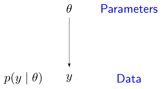
Graphically, the DGP can be represented using the language of directed acyclical graphs (DAGs); in a DAG, variables are represented as nodes and links between them are represented as arrows. For instance, Figure 1.1 shows an alleged DGP in which the observed data \(y\) depend probabilistically on a parameter \(\theta\). This dependence is expressed through the distribution \(p(y\mid\theta)\), which is used to describe the sampling variability for the observable data.
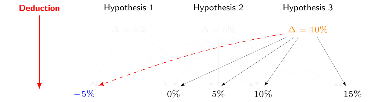
Standard (frequentist and maximum likelihood) procedures fix the working hypotheses and, by deduction, make inference on the observed data. The main consequence of this approach to statistical inference is that the hypotheses, or the features of the DGP (i.e. the parameters), are always assumed as fixed quantities. We generally do not know their value, but to a non-Bayesian, there is no uncertainty about it – the only source of uncertainty in our modelling is due to sampling variability in the data we have observed, or that we might observe in the future.
Often, statistical textbooks tend to conflate the main ideas underpinning the “frequentist” approach to statistical inference (championed among others by Jerzy Neymann and Egon Pearson) with the “likelihood” approach (almost single-handedly devised by Ronald Fisher). The two are in fact quite separate and the history of Statistics is actually full of heated exchanges between frequentists on one side and, mainly, Fisher on the other, to strongly argue over the supremacy of either philosophies1.
As it happens, Fisher was able to dress up his maximum likelihood theory so as to uphold the basic frequentist features and thus the maximum likelihood estimator is almost universally optimal from a frequentist perspective too. But there are fundamental differences in the two – with the common feature of rejecting the Bayesian philosophy. See Baio (2025) for more discussion of the distinctions in the three major schools of statistical inference, in the context of HTA.
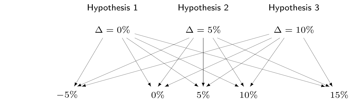
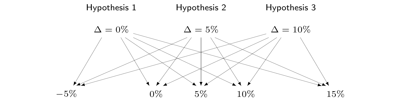
For example, in Figure 1.2 (a), we show an alleged DGP, in which there are three possible competing hypotheses; the first one assumes that the “true state of the world” is that some parameter \(\Delta\) (think of it as the difference in effectiveness for a given intervention) is equal to 0%; the second one assumes a small positive effect (\(\Delta=5\)%), while the third one assumes a large positive effect (\(\Delta=10\)%). Under either of these hypotheses, let us assume that there are a number of hypothetical observations we can make – for simplicity we assume a set of discrete outcomes, going from a minor negative result of \(-5\)% (indicating that the population given the treatment has slightly worse outcomes than that given the control), to a null outcome (0%), all to way to a very large positive observed effect of \(+15\)%.
Under a frequentist/maximum likelihood approach, statistical inference is concerned with questions such as
If my working hypothesis (e.g. that the true treatment effect is large, say \(\Delta=10\)%) is true, what is the probability of randomly selecting the data that I actually observed (e.g. a difference in outcome of \(-5\)%)?
If this probability is small, then we deduce weak support of the evidence to the hypothesis. In other words, the objective is to assess \(\Pr(\mbox{Observed data}\mid \mbox{Hypothesis})\). In reality (as shown in Figure 1.2 (b)), we cannot observe all possible datasets – say that the one actually realised is \(-5\)%. Nonetheless, we use the sampling variability that describes the probability of observing each one of the many possible data, under the conditions specified by a given DGP to quantify the weight of the evidence in favour of each competing hypothesis for the DGP. This is directly relevant for standard frequentist/maximum likelihood summaries, e.g. \(p\)–values, confidence intervals, etc. Crucially, this process also involves a comparison with data that could have been observed, but have not.
Example 1.1. Significance testing. Consider the classical example of significance testing applied to a “two-sample problem”, which we may represent using the following distributional assumptions: \[y_{10},\ldots,y_{n_{0}0}\stackrel{iid}{\sim}\text{Normal}(\mu_0,\sigma^2_0) \qquad \text{ and } \qquad y_{11},\ldots,y_{n_{1}1}\stackrel{iid}{\sim}\text{Normal}(\mu_1,\sigma^2_1),\] where, in general, \[ y\sim\text{Normal}(\mu,\sigma) \qquad \Rightarrow \qquad p(y\mid \mu,\sigma)=\frac{1}{\sigma \sqrt{2\pi}}\exp\left(-\frac{1}{2}\left(\frac{y-\mu}{\sigma}\right)^2\right). \tag{1.4}\]
In a case such as this, we may specify a “null” hypothesis as \(H_0: \mu_1=\mu_0\), or alternatively (and equivalently!) \(H_0: \delta=\mu_1-\mu_0=0\) – i.e. that there is “no treatment effect” at the population level.
Using some basic Normal theory, we can construct an estimator for the difference in the treatment effect \(\hat\delta=D=\bar{Y}_1-\bar{Y}_0\) and derive that \[\begin{eqnarray*} D = \bar{Y}_1-\bar{Y}_0 & \sim & \text{Normal}\left(\mu_D,\sigma^2_D\right) \\ & \sim & \text{Normal}\left( \mu_1-\mu_0, \frac{\sigma^2_0}{n_0}+\frac{\sigma^2_1}{n_1} \right) \end{eqnarray*}\] and estimating \(\sigma^2_D\) using the sample variance \[\begin{eqnarray*} S^2_D& = &\frac{S^2_0}{n_0}+\frac{S^2_1}{n_1} \\ & = & \frac{n_0}{n_0-1}\sum_{i=1}^{n_0} (Y_{i0}-\bar{Y}_0)^2 + \frac{n_1}{n_1-1}\sum_{i=1}^{n_1} (Y_{i1}-\bar{Y}_1)^2 \end{eqnarray*}\] derive the distribution of the “test statistic” \[ T=\frac{D-\delta}{\sqrt{S^2_D}} \sim \mbox{t}(0,1,n-1) \] where \[ y\sim\text{t}(\mu,\tau,\nu) \quad \Rightarrow \quad p(y\mid\mu,\tau,\nu)=\frac{\Gamma\left(\frac{\nu+1}{2}\right)}{\Gamma\left(\frac{\nu}{2}\right)}\sqrt{\frac{\tau}{\nu\pi}} \left(1 + \frac{\tau}{\nu}\left(y-\mu\right)^2\right)^{-\frac{\nu+1}{2}} \tag{1.5}\] indicates a t distribution with mean \(\mu\), precision (a measure of inverse variance) \(\tau\) and degrees of freedom \(\nu\).
Suppose that for the specific case at hand, the sample values and estimates are \[\begin{eqnarray*} n_0 = 80; & \qquad & n_1 = 78; \\ \bar{y}_0 = 25.12; & \qquad & \bar{y}_1 = 32.58; \\ S^2_0 = 355.85; & \qquad & S^2_1 = 376.88. \end{eqnarray*}\] Given these numbers, we can compute the observed value for the estimate of the true difference in the two means \(d=7.46\) and the estimate for its variance \[\begin{eqnarray*} s^2_D = \frac{s^2_0}{n_0} + \frac{s^2_1}{n_1} & = & \frac{355.85}{80} + \frac{376.88}{78} \\ & = & 4.45 + 4.83 = 9.28. \end{eqnarray*}\] Under the null hypothesis, the observed test statistic is \[ t = \frac{d-0}{\sqrt{s^2_D}} = \frac{7.46}{3.05} = 2.45. \]
The fundamental idea underpinning significance testing is that, if the null hypothesis were true, then we would expect the observed value \(t\) of the test statistic \(T\) to be fairly “central” in the range of its sampling distribution. In other words, we can use the tail-area probabilities under the sampling distribution \(p(t\mid\theta,H_0)\) to find the chance of observing a result “as extreme as, or even more extreme than” the one that actually obtained in the current data.
Intuitively, if \(t>\mbox{Med}(T)\), i.e. the observed value of \(t\) is “larger than normal”, we would be looking at even larger values; conversely, if \(t\leq \mbox{Med}(T)\), “even more extreme” values would be in fact smaller than that observed.
In the present case, we can use R to compute the \(p\)–value \(\Pr(T>t\mid \theta,H_0)\); Figure 1.3 shows this as the grey area to the left of the observed value \(t=2.45\).
pt(q=t,df=n-1,lower.tail=FALSE)[1] 0.007697083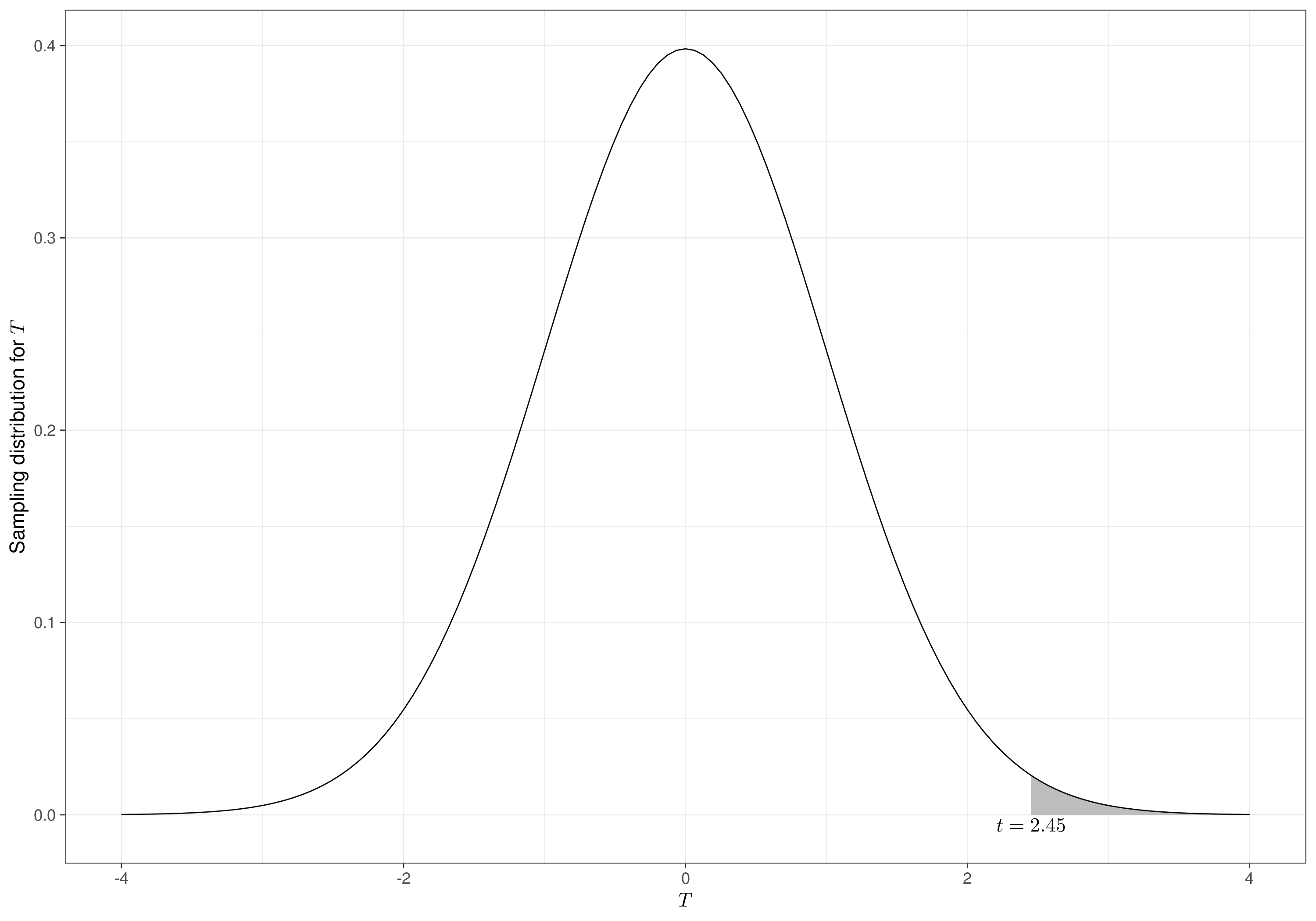
The interpretation of the \(p\)–value in terms of assessing the probability of observing something as extreme as, or even more extreme than the data actually observed (or, in other words, as a tail-area probability) is clearly a mouthful and a slightly subtle concept. The reason why we need to use such a convoluted phrasing is that, when dealing with continuous data, the sampling distribution does not really represent a probability, but rather a density. So, it is impossible to quantify the strength of the evidence just in correspondence of the observed value for the test statistic.
One criticism associated with this (inevitable!) choice is that the strength of the evidence (or, in other words, whether the observed data are consistent with the working hypothesis) depends on the data actually observed, as well as on data (“even more extreme”) that might be – but have not been – observed. In addition to this, by its own nature, it is possible that the same \(p\)–value is computed for a very small and a very large study; the conclusion in terms of strength of the evidence would be identical, without distinction of the underlying sample size (Goodman, 1999).
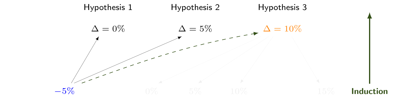
The Bayesian philosophy proceeds exactly in the opposite direction, i.e. by fixing the value of the observed data and, by induction, making inference on unobservable hypotheses. Figure 1.4 (a) shows the same DGP described in Figure 1.2 (a): there are three possible hypotheses that can generate a number of hypothetical observed data. However, from a Bayesian perspective, once the one and only dataset is observed (in this case with a value of \(-5\)%, highlighted in Figure 1.4 (b)), there remains no uncertainty over the observations – this is why every other hypothetical outcome is greyed out in Figure 1.4 (b). The sampling mechanism is relevant to get us there, but once we know what the data are, the only relevant question thus becomes
What is the probability of my working hypothesis, given the data I observed?
If this is less than the probability associated with other competing hypotheses, then we can deduce weak support from the evidence to the hypothesis. This implies that the Bayesian procedure is interested in assessing \(\Pr(\mbox{Hypothesis}\mid\mbox{Observed data})\) and that, crucially, unobserved data have no role in the inference.
The posthumous work of Reverend Thomas Bayes (1763) is considered the origin of what we now call “Bayesian” approach. However, interestingly, Fienberg (2006) suggests that it was not until the 1950s that the term “Bayesian” came to be used, with Ronald Fisher, one of the most anti-Bayesians of the time, among those potentially credited with the invention of the term (other, perhaps more likely candidates are Dennis Lindley and Irving John Good, who were much more of a Bayesian persuasion…).
As mentioned by Fienberg (2006)
…In current statistical language, Bayes’ paper introduces a uniform prior distribution on the binomial parameter, \(\theta\) reasoning by analogy with a “billiard table” and drawing on the form of the marginal distribution of the binomial random variable…
In fact, quoting Stigler (1982), Fienberg (2006) argues that
…Bayes intended his results in a rather more limited way than would modern Bayesians.
and that the actual development of what we generally refer to as “Bayesian” modelling is perhaps more to do with the later (and, apparently, independent) work of Pierre Simon Laplace (1812) – see also Section 2.2.1.
Bertsch McGrayne (2011) presents an engaging account of the historical impact of Bayesian modelling, including on Alan Turing’s work on “cracking the Enigma Code”, the complex system of encrypted messages used by the German Army in World War Two, which also led to the foundations of modern computers.
In a Bayesian context, we need to specify a full probabilistic model that applies to everything over which we have uncertainty – be it sampling variability (e.g. the data that we may have observed or that we may be able to observe in the future) or epistemic uncertainty, e.g. the parameters of the model (which in fact we are never in a position of observing – the parameters may possess no physical meaning but just be a mathematical construction that helps us define the model!) or some hypothesis that describes the form of the alleged DGP.
In fact, much as in the frequentist/likelihood context, even from a Bayesian perspective it is perfectly possible that parameters may in fact have a “true”, underlying, immutable and fixed value; however, because we do not know this value, the Bayesian view is to model this lack of knowledge by associating a suitable probability distribution. This means that, to a Bayesian, probability is the only language to assess any form of imperfect information or knowledge: there is no need to distinguish between “probability” and “confidence”. To be able to work in this context, however, before even seeing the data, we need to identify a suitable probability distribution to describe the overall uncertainty about the data \(\boldsymbol{y}\) and the parameters \(\boldsymbol{\theta}\), which we can factor as \[p(\boldsymbol{y},\boldsymbol{\theta}) = p(\boldsymbol{\theta})p(\boldsymbol{y}\mid\boldsymbol{\theta}) = p(\boldsymbol{y})p(\boldsymbol{\theta}\mid \boldsymbol{y}),\] from which we can directly derive Bayes’ theorem \[ p(\boldsymbol{\theta}\mid \boldsymbol{y}) = \frac{p(\boldsymbol{y}\mid\boldsymbol{\theta})p(\boldsymbol{\theta})}{p(\boldsymbol{y})}. \tag{1.6}\] The denominator in the right-hand side of Equation 1.6, the marginal distribution for the data \[\displaystyle p(\boldsymbol{y})=\int p(\boldsymbol{y}\mid\boldsymbol{\theta})p(\boldsymbol{\theta})d\boldsymbol{\theta}, \tag{1.7}\] also referred to as (prior) predictive distribution, does not depend on \(\boldsymbol{\theta}\) and can be seen as a normalising constant, ensuring that the left-hand side integrates to 1 (and so is a proper probability distribution).
For this reason, we can also rewrite Equation 1.6 as \[p(\boldsymbol{\theta}\mid \boldsymbol{y}) \propto p(\boldsymbol{y}\mid\boldsymbol{\theta})p(\boldsymbol{\theta}) \propto \mathcal{L}(\boldsymbol{\theta}\mid\boldsymbol{y})p(\boldsymbol{\theta}),\] where \(\mathcal{L}(\boldsymbol{\theta}\mid\boldsymbol{y})\) is the likelihood function – this is derived from the sampling distribution, but taken as a function of the model parameters, for the fixed, observed value of the data (see Note 1.3, below). The posterior distribution is thus proportional to the product of the prior and the likelihood.
Sometimes, statistical texts tend to conflate the concept of sampling distribution \(p(y\mid\theta)\) with that of likelihood function \(\mathcal{L}(\theta\mid y)\), because these two functions are mathematically similar, since the latter is derived from the former. Nonetheless, they are not quite the same…
Consider, for instance, a model \(y\sim \text{Normal}(\mu,\sigma)\), where the sampling distribution is defined as in Equation 1.4. Assume also, for simplicity, that the standard deviation is known and that the only relevant parameter is the mean \(\mu\); in this case, the likelihood function is defined with respect to \(\mu\) only and every term in Equation 1.4 that does not depend on \(\mu\) should be just dropped, leading to \[\mathcal{L}(\mu\mid y,\sigma) = \exp\left(-\frac{1}{2\sigma^2}(y-\mu)^2\right)\] (note that we cannot discard the scaling factor \(1/\sigma^2\) inside the exponential, as this changes the shape of the likelihood function and thus affects the main parameter \(\mu\)).
The likelihood function, in general, does not integrate to 1 (as does any proper sampling distribution) and thus, from a purely mathematical point of view, the two are just not the same – there are even more extreme cases in which the data are discrete and the parameter is continuous (see Equations 1.16 and 2.3, for instance).
For these reasons, the phrasing “Normal likelihood” is not really meaningful: the likelihood function derived from a model where the sampling distribution is described by a Normal distribution is just not the same as the Normal density. It depends on a different variable (for different known constants) and, in general, it has a different support.
Generally speaking, the choice of the prior distribution may exert considerable impact on the inferential process. This is particularly true when the evidence provided by the observed data is non-definitive – examples include cases with limited follow-up, or small sample sizes.
On the one hand, this is often seen as a critical part of a Bayesian analysis, because it is unsettling that, despite observing or using the exact same data, two researchers using widely different prior distributions may end up with substantially different inferences. However, on the other hand, this is not entirely surprising, in the case where the information provided by the data is limited – my prior distribution may lead to very different conclusions than yours, simply because we do not have enough in the data to converge towards a common assessment and so where we start from (our contextual background knowledge) does matter and the inference is strongly sensitive to that.
Example 1.2. Two experts. Consider a situation in which two experts are called upon to provide information about the population effectiveness of a particular health intervention. The first one (\(E_1\)) indicates that, in their considered opinion, the probability that a random individual is cured by receiving that intervention is around 20% and that if they had to provide some kind of range for this, their considered opinion would be between 5% and 40%, approximately.
The second expert (\(E_2\)) strongly disagrees and, in their considered opinion, the intervention is much more likely to work; \(E_2\) estimates an average effectiveness around 80% and, if they were forced to provide a range of likely values, they would say something like 60% to 95%.
You, the Bayesian statistician, take this information and manage to translate it into two suitable prior distributions, \(p_1(\theta)\) and \(p_2(\theta)\). The underlying uncertainty is summarised in the top panel of Figure 1.5, which highlights the very different starting position of the two experts (how you actually map the assumptions to distributions is not important just yet, but we return to this in the next sections).
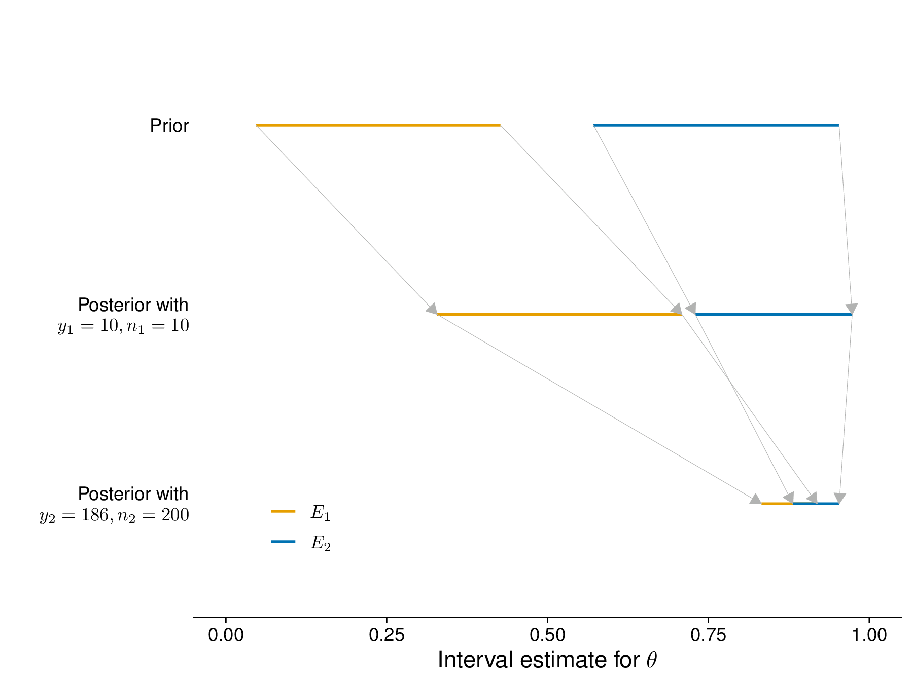
Imagine that we manage to observe a sample of \(n_1=\) 10 individuals, representative of the target population and observe whether the intervention has an effect on them. As it happens, in the sample, \(y_1=\) 10 actually have a positive response. You perform a Bayesian analysis and obtain the two posterior distributions in the middle panel of Figure 1.5, with which you revise your uncertainty – again, how you actually obtain the posteriors is not important, for now. As it is possible to see from the middle panel of Figure 1.5, the data do change the prior opinions to rather different extents: \(E_2\) was probably more “calibrated” and their assessment is pretty much in the right “ball-park” as far as this first set of \(n_1\) data is concerned; for \(E_1\), the prior assessment was rather far from the evidence and yet the posterior gets pulled “in the right direction”.
With very different prior opinions and little information in the data, the two experts still differ in their judgement and \(E_1\) is still not convinced that they may be wrong about this (it’s probably a man…). To definitively resolve the question, you manage to obtain a very large sample of \(n_2=\) 200 people, of which \(y_2=\) 186 have a positive response – these new data are much more convincing. You replicate your analysis and produce a new set of posterior distributions, shown in the bottom panel of Figure 1.5. Because of the very strong signal provided by the data, now the two experts have effectively coinciding opinions – the two intervals overlap.
As consistent evidence accrues pointing in the same direction, it matters less and less where the two experts were starting from: when modelled rationally through Bayesian updating, the posterior inference tends to coincide, given enough and consistent information coming from the data.
As is perhaps obvious from Example 1.2, any form of prior distribution is in fact based on some background (contextual) information, available to the experimenter. We may indicate this (possibly qualitative, ideally quantitative) information as \(\mathcal{B}\) and thus, the prior distribution should really be described as \(p(\bf{\theta}\mid\mathcal{B})\), which means that if data \(\boldsymbol{y}\) become available, our uncertainty will be updated to \[p(\boldsymbol{\theta}\mid \mathcal{B},\boldsymbol{y}) = \frac{p(\boldsymbol{\theta}\mid\mathcal{B})p(\boldsymbol{y}\mid\boldsymbol{\theta})}{p(\boldsymbol{y})}.\]
This notation clarifies that, to a Bayesian, everything is really conditional to whatever is the current state of science. In general, it is possible that \(\mathcal{B}\) does contain very little information and therefore \(p(\theta\mid\mathcal{B})\) is very vague and subject to a large variance/uncertainty. In that case, it is even more important to present substantial sensitivity analysis to assess the impact of choices in how the contextual knowledge is modelled on the inference process – although when the prior is vague and the amount of information in \(\boldsymbol{y}\) is large and consistent, it is possible that it “supersedes” that included in \(\mathcal{B}\) and so, for all intents and purposes, the posterior basically depends on \(\boldsymbol{y}\) only (and it sort of “forgets” the input provided by the background, contextual information \(\mathcal{B}\), as shown in Example 1.2).
In addition, the notation and discussion above clarify that, from a purely Bayesian perspective, we can elicit all sorts of information to construct the prior distribution: we may look at events for which there are masses of existing data and use these to form our prior; or, at the other end of the spectrum, base the prior solely on our subjective knowledge. Both are valid options, to a Bayesian. Whenever possible, of course, we should try and use “hard” evidence to form our prior (e.g. existing studies, registries, literature, etc.).
While the discussion above indicates that in reality we should always describe the prior as a conditional distribution, given the background knowledge \(p(\theta\mid\mathcal{B})\), almost invariably we favour simplicity over pedantic completeness2 and just write \(p(\theta)\), thus dropping reference to \(\mathcal{B}\) altogether.
Example 1.3. Covid-19 testing. Imagine that, for a dreadful moment, you are taken back to the Winter of 2020, in the midst of the second Covid-19 pandemic wave. You do not feel very well and so you decide to get tested. Given the evidence and knowledge \(\mathcal{B}\) that, by then, was piling up, your doctor is able to consider the situation shown in Figure 1.6.
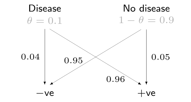
The assumptions encoded in the DAG are that
Given these assumptions, if your test comes up negative, there is fairly strong evidence against the hypothesis that the true status is “Disease” – this roughly implies a \(p\)–value of 0.04.
But how prevalent is Covid in the population, at the time of your test? Clearly, you should consider this contextual information when assessing the significance (in plain English, rather than in statistical parlance) of this result. One way to do it is to consider Bayes’ theorem (adapting Equation 1.6) and combine the information from the data with our contextual knowledge \[\Pr(\text{Disease} \mid \text{-ve}) = \frac{\Pr(\text{Disease})\Pr(\text{-ve} \mid \text{Disease})}{\Pr(\text{-ve})},\] where, by the law of total probabilities (of which Equation 1.7 is a generalisation), \[\Pr(\text{-ve}) = \Pr(\text{Disease})\Pr(\text{-ve} \mid \text{Disease}) + \Pr(\text{No disease})\Pr(\text{-ve} \mid \text{No disease}).\] Note that, as far as we are considering events (rather than random variables), Bayes’ theorem is really not controversial at all – it is a simple application of the basic definitions for conditional probabilities, based on Kolmogorov’s axioms (which are the cornerstone of the frequentist philosophy of probability too).
For example, suppose that from extensive surveys that were conducted at the time, the doctor is reasonably confident that \(\Pr(\mbox{Disease})=\theta\approx 0.1\). The evidence from the data alone tells us that the observed result is extremely unlikely under the hypothesis of “Disease”; but this is strongly dependent on the context, as provided by the prior knowledge/epistemic uncertainty, as shown in Figure 1.7.
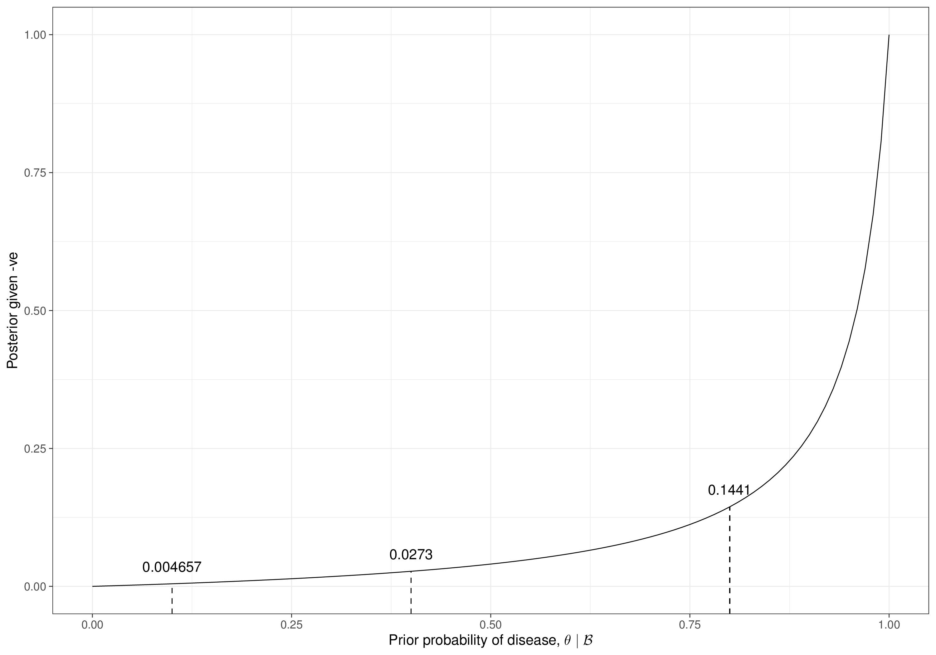
As is obvious, if we assumed that \(\theta=0\) (which would mean that nobody has Covid, in the reference population), then the negative test would not be very exciting and the posterior probability would also be 0. Similarly, if everyone had Covid, even the negative result would not be able to cheer you up – your posterior probability of having Covid would still be 1, because everyone has it.
For any other possible value of the prior probability of the disease, then there is a gradation and the evidence provided by the negative test moves the prior to a very different posterior – for instance, if 80% of the population had Covid, the fact that you tested negative would still make your probability of having it too at around 14%. In the alleged situation where around 10% of the population has Covid, this means that your probability of also being infected, having tested negative, is around 0.0046 – much smaller (and fundamentally different in nature!) than the nominal \(p\)–value, without direct and explicit reference to the background information.
The discussion above also highlights the cyclical nature of Bayesian inference: we start from the contextual knowledge \(\mathcal{B}\) to form our current state of uncertainty on some idealised feature of a DGP, \(\boldsymbol{\theta}\), in terms of a prior distribution \(p(\boldsymbol{\theta}\mid\mathcal{B})\). We then observe some data \(\boldsymbol{y}\), which we are willing to assume as conforming with the alleged DGP described by \(\boldsymbol{\theta}\) and use Bayes’ theorem to update our state of knowledge to a posterior, which for simplicity we may indicate as \(p(\boldsymbol{\theta}\mid\boldsymbol{y})\) – again, dropping for simplicity the initial, background information \(\mathcal{B}\), which by now may be much less influential, given the observation of \(\boldsymbol{y}\).
We are not done, though; in fact, the process is only about to start over: this time, our current contextual/background information is described by \(p(\boldsymbol{\theta}\mid\boldsymbol{y})\). To put it like Lindley (1972), “Today’s posterior is tomorrow’s prior” and if we observe new data \(\boldsymbol{y^*}\), the process will be repeated to obtain a new, updated posterior \[p(\boldsymbol{\theta}\mid\boldsymbol{y,y^*})=\frac{p(\boldsymbol{\theta}\mid\boldsymbol{y})p(\boldsymbol{y^*}\mid\boldsymbol{\theta})}{p(\boldsymbol{y^*})}.\]
For all the prominence given to the model parameters, in reality these are merely mathematical constructions that we are willing to “make up” to provide an easier description of a potentially very complicated DGP. In fact, a truly “hard-core” Bayesian would not really put so much emphasis on parameters and the prior/posterior distribution – what they would be really interested in is actually the predictive distribution of Equation 1.7.
In general terms, however, when we use a parametric model to describe a sampling distribution and thus a DGP, we make use of a mathematical formulation \(p(\boldsymbol{y}\mid\boldsymbol{\theta})\); typically, \(\boldsymbol{\theta}\) represents a vector of original-scale parameters – these are used to index the mathematical function \(p(\cdot)\). As an example, consider the Gamma distribution of Equation 1.2, which is defined as a function of a shape \(\eta\) and a rate \(\lambda\). Neither of these parameters has a special physical meaning – they are just quantities we make up to create a functional form that is good enough to describe the DGP we have in mind (a positive, continuous, skewed variable).
In some other cases, the parameters \(\boldsymbol{\theta}\) are much easier to interpret: for instance, in the case of a variable whose sampling distribution is modelled using the Normal distribution of Equation 1.4, the vector of parameters \(\boldsymbol{\theta}=(\mu,\sigma)\) has a very clear and direct interpretation as the mean and the standard deviation. These quantities are original-scale parameters, ensuring that the mathematical properties of the resulting density function align with the assumptions we want to encode (symmetry, unbounded range, continuous support). But they also have the role of natural-scale parameters, because they have a direct physical interpretation of which we can make sense.
Interestingly, in essentially all parametric models we encounter, it is possible to relate the original- to the natural-scale parameters: for example, in the Normal case, they coincide, as mentioned above; in the Gamma case, we can use the mathematical properties of the Gamma density and derive that if \(y\sim\text{Gamma}(\nu,\gamma)\), then \[\mbox{E}[Y]=\mu=\frac{\nu}{\gamma} \qquad \mbox{and} \qquad \mbox{Var}[Y]=\sigma^2=\frac{\nu}{\gamma^2},\] which implies, using simple algebra, that \[\gamma=\frac{\mu}{\sigma^2} \qquad \mbox{and} \qquad \nu=\frac{\mu^2}{\sigma^2}. \tag{1.8}\]
This consideration is very helpful when trying to elicit genuine information \(\mathcal{B}\) to form a prior distribution: it may be very awkward to think in terms of shape and rate (of which we would most likely struggle to make sense, from a physical point of view); but it may be much simpler to think in terms of the question
What do we know/can we expect as the most likely value for the mean and standard deviation of the variable \(Y\), given current/contextual/background information?
But if we can derive a relationship such as that of Equation 1.8 (which, in general, we can) between the original- and natural-scale parameters, then we can define a prior for the natural-scale parameters and then derive the implied prior for the original-scale parameters.
Mapping a probability distribution from one scale to another is often possible analytically, i.e. we can work out the mathematical relationship and determine the exact form of the required distribution for any re-parameterisation in which we are interested. In many other cases, this is either too complicated or even impossible; however, we can still resort to numerical approximation – the most popular option is to use Monte Carlo simulations.
Using simulation methods to perform inferential tasks is not a purely Bayesian feature. In a frequentist/maximum likelihood approach, we can still use simulations, e.g. bootstrap (Efron and Tibshirani, 1994) to approximate interval estimates or evaluate the “long-run” properties of specific estimators. This is very popular also in health technology assessment: see Section 4.3.
Arguably, though, in the last 30 years or so, inference by simulations has become ubiquitous especially within a Bayesian context and has fundamentally contributed to its applicability and success.
The main idea is that if we are able to simulate a large number of values from a probability distribution, then we can use these simulations to summarise it; for instance, the mean of a continuous random variable \(Y\) defined on the range \(\mathcal{Y}\) is computed as the integral \[\text{E}[Y] = \int_{\mathcal{Y}} yp(y\mid\theta) dy.\] When this is too complicated, or does not have a closed form solution, or simply we cannot be bothered to sit down and “do the maths”3, we can approximate this integral by simulating a large number \(S\) of values from \(p(y\mid\theta)\), say \(y^{(1)},\ldots,y^{(S)}\) and then use these to compute \[\text{E}[Y] \approx \sum_{s=1}^S \frac{y^{(s)}}{S}.\]
In fact, given the sample of Monte Carlo (MC) simulations \(y^{(1)},\ldots,y^{(S)}\), we can use them to summarise any feature of the underlying distribution, in the form of a given function \(g(y)\) – provided we have enough simulations, so as to reduce the approximation error. For instance, we can use the sample (simulated) quantiles to give an indication of interval estimates, as the following R code demonstrates.
# Simulates a sample of S values from y ~ Normal(0,1)
S=100000
y=rnorm(S,0,1)

# Computes the 2.5%  and 97.5% quantile; these are the points y_{0.025} and
# y_{0.975} such that Pr(Y<=y_{0.025})=0.025 and Pr(Y<=y_{0.975})=0.975
quantile(y,c(0.025,0.975))
2.5% 97.5%
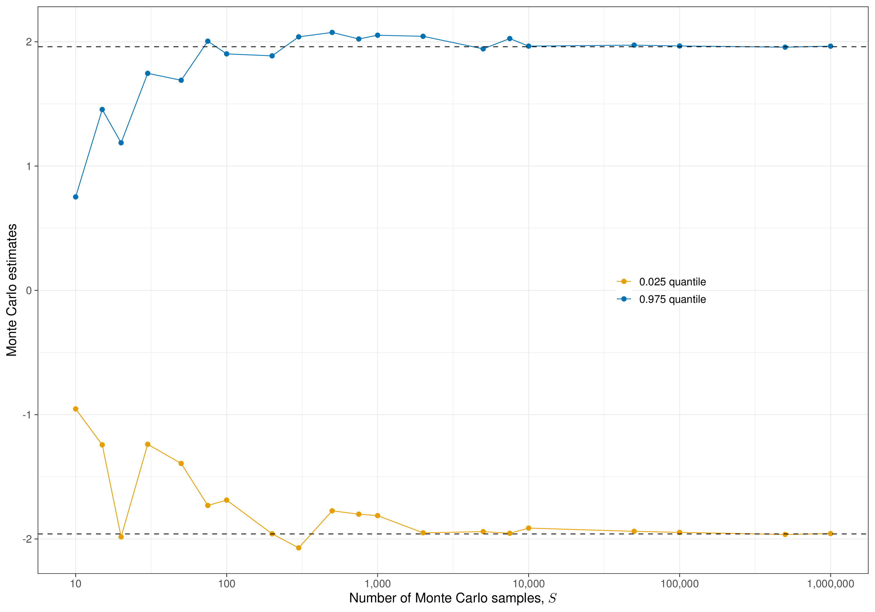
-1.969646 1.970057 The accuracy (or the “Monte Carlo error”) of the estimate depends, obviously, on the sample size, as highlighted in Figure 1.8: if we only sample \(S=10\) values from a \(\text{Normal}(0,1)\), then the approximation to the analytic quantiles (\(-1.959964\) and \(1.959964\)) is pretty coarse, due to the sampling variability intrinsic in the process. However, increasingly large MC samples get closer and closer to the “true” values – in many circumstances, 1000 MC samples are enough, but this varies and the choice of the number of simulations usually requires some care (see Section 2.3.2). Having a running series of results, as in Figure 1.8 is often very helpful to assess the “stability” of the simulation process – when continuing to increase \(S\) does not vary substantially the overall estimate, we can be fairly confident about the results.
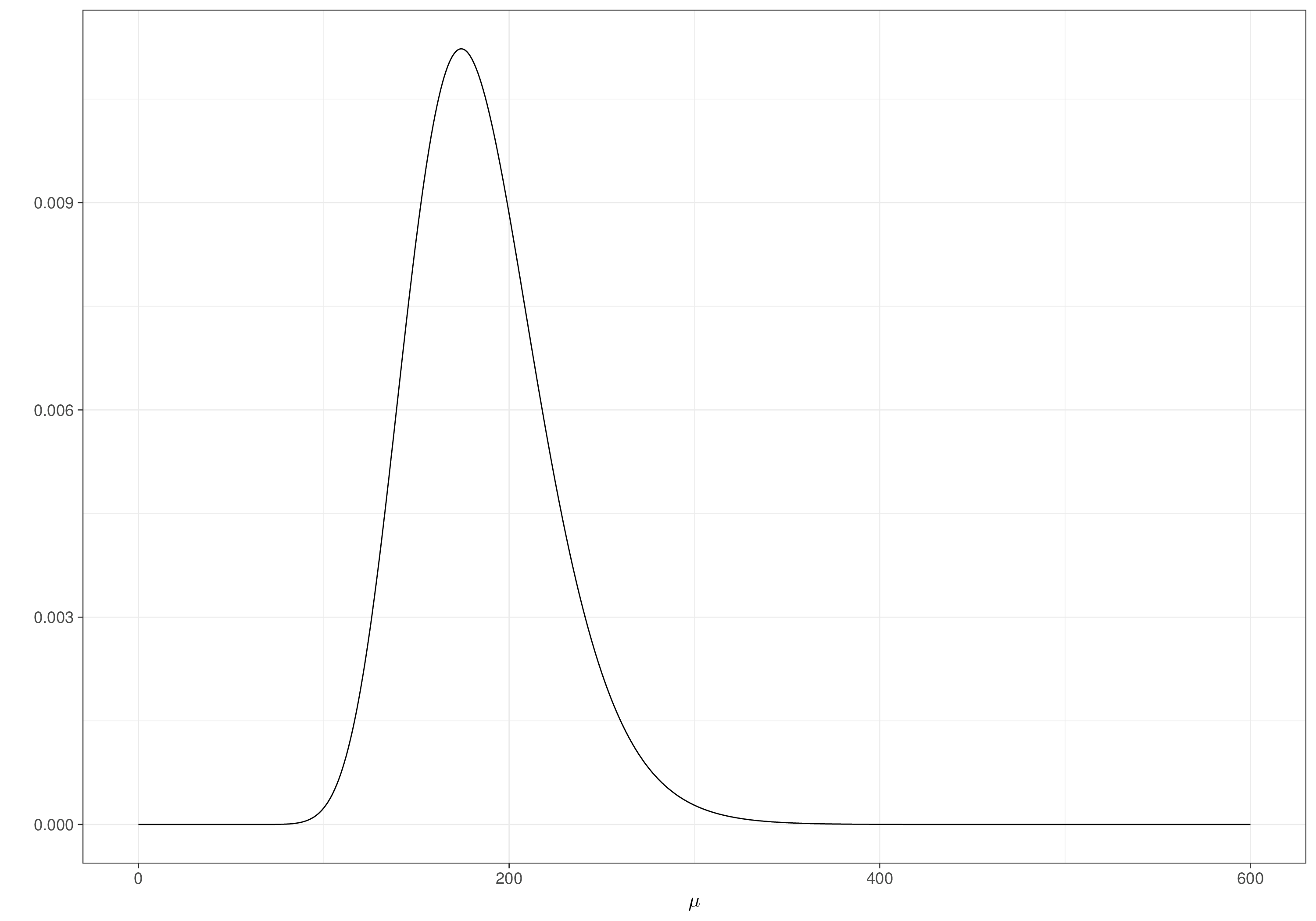
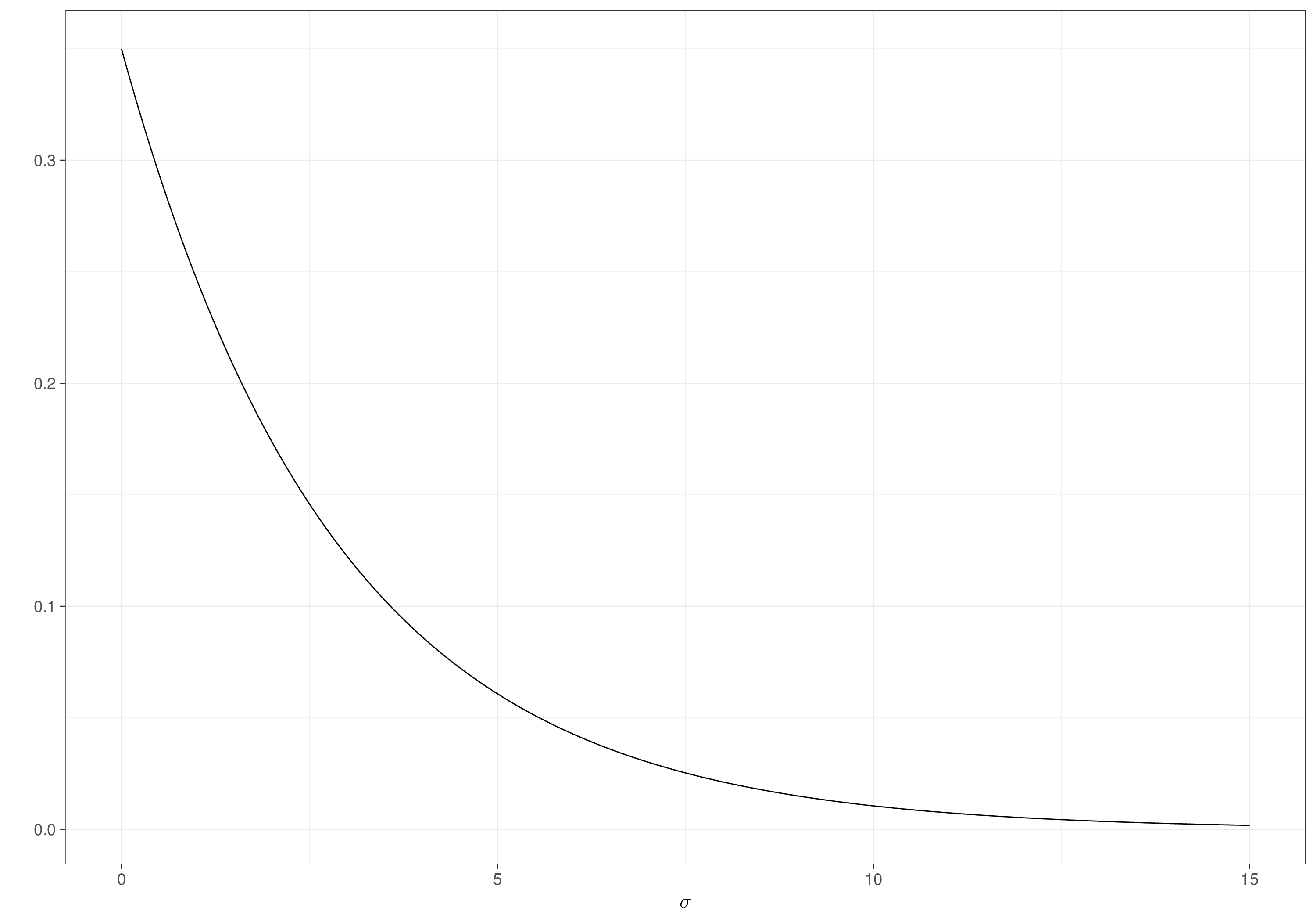
Back to the example introduced in Section 1.2.3, if, perhaps using some background knowledge about the likely ranges of the mean and standard deviation for the underlying variable, we set the priors on the natural-scale as \(\mu\sim\text{log-Normal}(5.2,0.2)\) and \(\sigma\sim\text{Exponential}(0.35)\), where, in general, \[
y\sim\text{log-Normal}(\eta,\lambda) \qquad \Rightarrow \qquad p(y\mid \eta,\lambda)=\frac{1}{y\sqrt{2\pi \lambda^2}}\exp\left( -\frac{(\log y-\eta)^2}{2\lambda ^2}\right)
\tag{1.9}\] and \[
y\sim\text{Exponential}(\theta) \qquad \Rightarrow \qquad p(y\mid\theta)=\theta \exp\left(-\theta y\right),
\tag{1.10}\] we can then use MC simulation to derive the implied priors on the original-scale parameters \((\eta,\lambda)\), for instance using the following R code.
# Loads relevant packages
library(tibble)  # management of datasets
library(ggplot2) # graphs

# Simulate values from the prior on the *natural* parameters
mu=rlnorm(10000,5.2,.2)
sigma=rexp(10000,.35)

# Transform the prior for the *original scale* parameters
gamma=sqrt(mu/sigma^2)
nu=mu*gamma

# Plots the resulting prior for eta and lambda
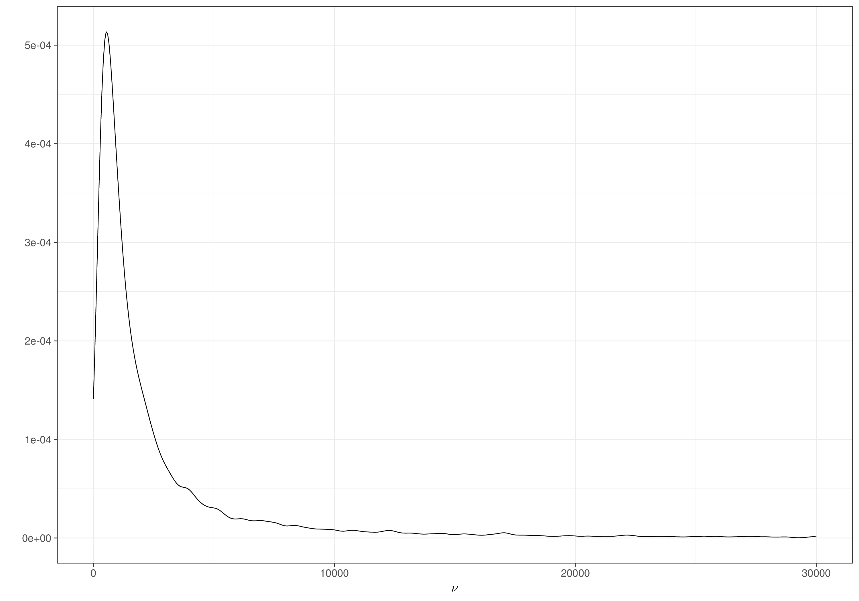
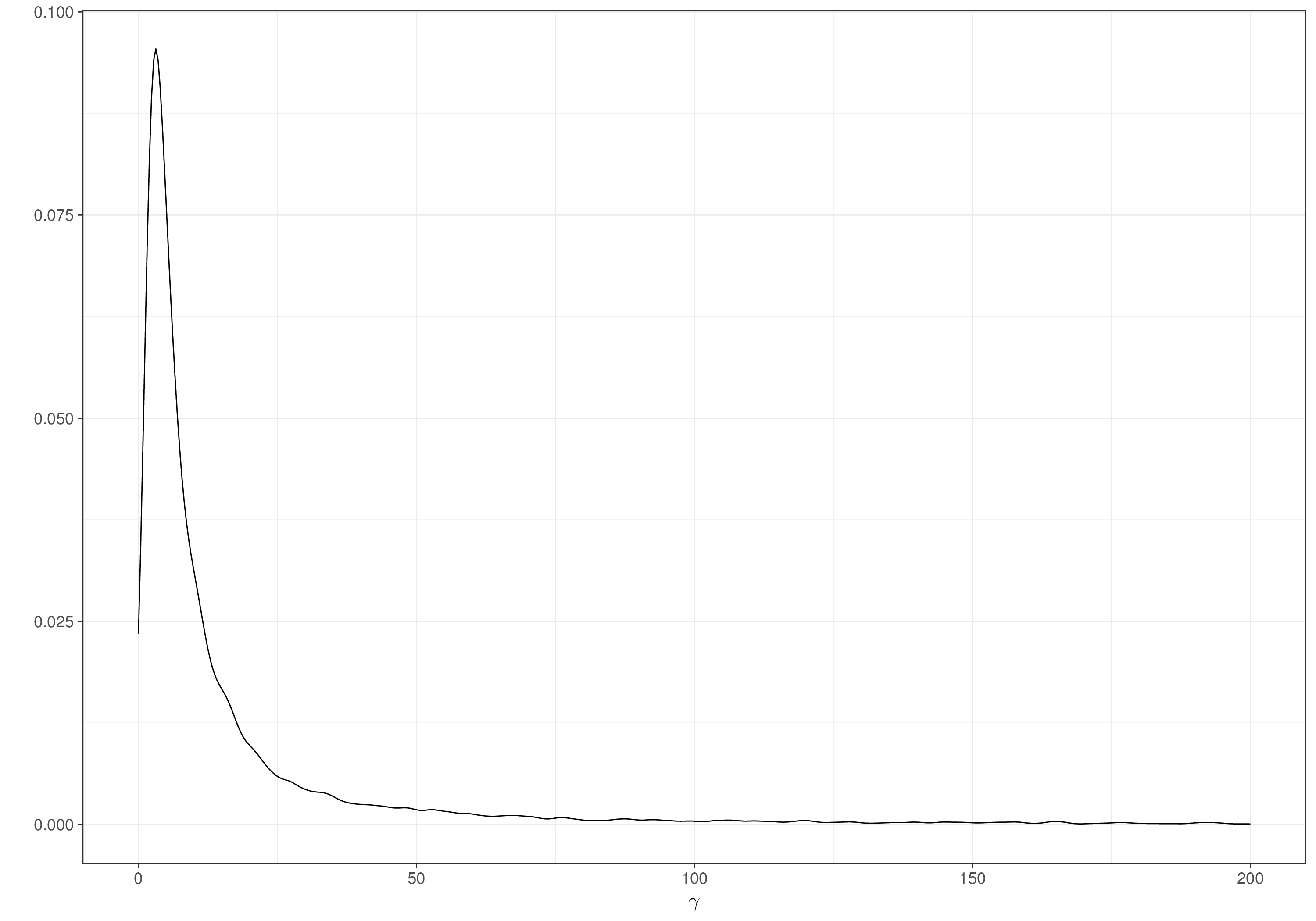
tibble(nu) |> ggplot(aes(nu)) + geom_density()
tibble(gamma) |> ggplot(aes(gamma)) + geom_density()In a sense, it does not matter what the resulting prior is for \(\nu\) and \(\gamma\) – we want the contextual information to make sense on the scale that we can think about in the first instance (\(\mu,\sigma\)). In fact, we probably do not know the close form of the resulting prior for \((\nu,\gamma)\), but we do not need this, as long as we can sample from \(p(\nu)\) and \(p(\gamma)\), which we can, using MC simulations.
Example 1.4. Drug (adapted and expanded from Spiegelhalter et al., 2004). Consider a drug that is being developed to reduce back pain. Even before we get to see any data from actual experimentation, we may have some contextual, background evidence \(\mathcal{B}\) to inform our “guess” at the drug’s effectiveness, indicated as \(\theta\), i.e. the probability that a random individual taking the drug manages to control their back pain. We may use expert opinion (e.g. the team of experiementers’ knowledge about the biology and pharmacodynamics of the molecule being tested), but also “hard” evidence, for instance obtained from population registers looking at the performance of existing drugs based on the same active principle, or small/pilot studies conducted by the company who are developing the drug.
For example, imagine that the experimenters are convinced that this particular drug is likely to be effective in combating back pain within a 20% to 60% range. The role of the statistician is to map this particular prior information into a suitable prior distribution.
We could interpret the prior information that “most of the probability mass lies between 0.2 and 0.6” by assuming that this basically identifies a symmetrical interval around the mean of the distribution, including something like 95% of the mass to mean “most of the probability”. Then, using some basic Normal theory, at least approximately, we can reasonably assume that \[\mu -2\sigma = 0.2; \qquad \mu+2\sigma=0.6; \qquad \mbox{and} \qquad \mu=\frac{0.6+0.2}{2}=0.4,\] from which we can derive \(\sigma=0.1\).
There are of course many ways to encode this knowledge into a suitable prior distribution for \(\theta\). Just as an example, we may start by considering a probability model that fits the physical properties of the parameter of interest: because \(\theta\) represents a probability (the proportion of people who will be relieved from back pain if taking the drug), then we know that it must take on values in the interval \([0; 1]\).
This consideration can help us select a suitable model – in this case, a natural candidate is the Beta distribution, which is defined in the range \((0,1)\) by a density \[ p(\theta\mid a, b) = \frac{\Gamma(a+ b)}{ \Gamma(a)\Gamma(b) } \,\,\theta^{a-1} (1-\theta)^{b-1}, \tag{1.11}\] where the mean and the variance are defined as \[\mu =\frac{a}{a+ b} \qquad \mbox{and}\qquad \sigma^2 = \frac{a b}{ (a+ b)^2 (a+ b+1)}. \tag{1.12}\] Back-solving for \(a,b\), we can derive \[ a = \mu\left(\frac{(1 - \mu)\mu}{\sigma^2} - 1\right) \qquad \mbox{and}\qquad b = (1 - \mu)\left(\frac{(1 - \mu)\mu}{\sigma^2} - 1\right ). \tag{1.13}\]
Setting \(\mu=0.4\) and \(\sigma=0.1\) and plugging these values in Equation 1.13 yields \(a=9.2\) and \(b=13.8\). In other words, at least approximately, a \(\text{Beta}(a=9.2, b=13.8)\) implies that most of its mass is included in the interval \([0.2;0.6]\) and that the mean is around \(0.4\). We can check this using Monte Carlo simulation, as with the following R code.
# Defines the number of simulations
nsim = 10000

# Then defines the prior distribution for theta
alpha = 9.2
beta = 13.8
theta = rbeta(n=nsim, shape1=alpha, shape2=beta)
The package bmhe (which is available from the GitHub repository at https://github.com/giabaio/bmhe_utils) provides a number of utility functions to process the output of Bayesian simulations. To install the package (which we will use throughout the book), it is possible to use either of the following commands:
# Installs the package 'remotes', that can be used to download packages
# off a GitHub repository (only need to run this command once)
install.packages(remotes)
# Uses 'remotes' to install the package from GitHub
remotes::install_github("giabaio/bmhe_utils")

# Or via the alternative repository at https://giabaio.r-universe.dev/
install.packages(
  "bmhe",
  repos=c("https://giabaio.r-universe.dev","https://cloud.r-project.org")
)Once bmhe is installed, we can then use its function stats() to summarise the prior distribution
# Produces summary statistics for the prior
bmhe::stats(theta)
mean sd 2.5% median 97.5%
0.40314978 0.09979373 0.21729833 0.40024981 0.60306573 and we can also visualise the prior in the form of a histogram, as in Figure 1.10.
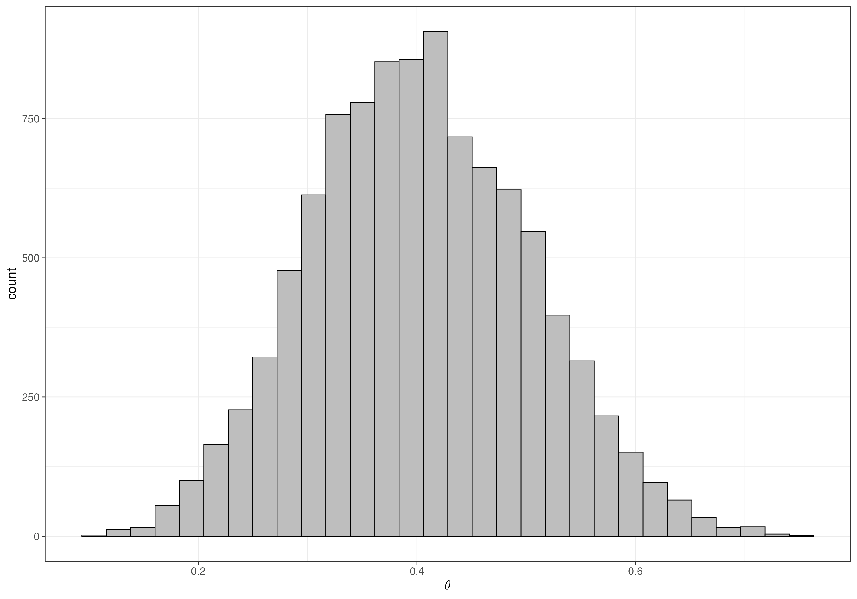
As we can see both visually and numerically, most of the mass is between around 20% and 60% (we already knew this – it was the reason why we set up this particular Beta prior). We can also specify prior probabilities associated to specific cut-off points: for example, it may be clinically relevant to report \(\Pr(\theta>0.5)\), which we can easily compute using the simulations from the prior, stored in the vector theta:
sum(theta>0.5)/length(theta)[1] 0.1742(note the use of the built-in function length() to characterise the number of values included in the vector theta, which is of course identical to the variable nsim).
As mentioned in Example 1.4, there is a fundamental distinction between the unique prior information that is available to us and the many ways in which we can decide to map it onto a prior probability distribution.
For example, we may decide to map the fact that “more or less 95% of the distribution lies between 0.2 and 0.6” onto a \(\text{Beta}(a=9.2,b=13.8)\) distribution, as discussed in Example 1.4. Or: we may decide that it is easier for us to work with Normal distributions – of course applying a Normal distribution to describe a variable that is, by definition, constrained in the \([0;1]\) interval is not fully appropriate. However, we may first transform the original parameter \(\theta\) to the \((-\infty; \infty)\) range, e.g. using the logit function and then use a suitable Normal distribution to describe our uncertainty on the logit scale: \[\phi = \text{logit}(\theta) := \log\left(\frac{\theta}{1-\theta}\right)\sim \text{Normal}(m,s).\]
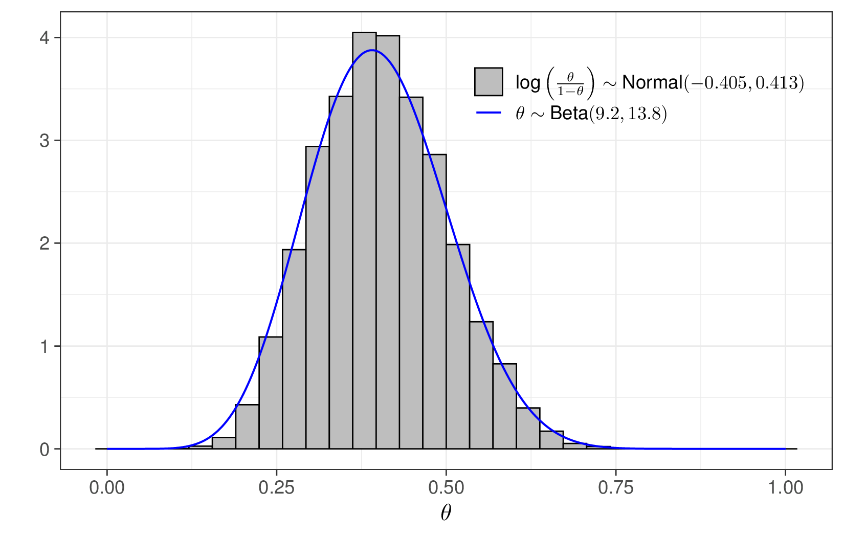
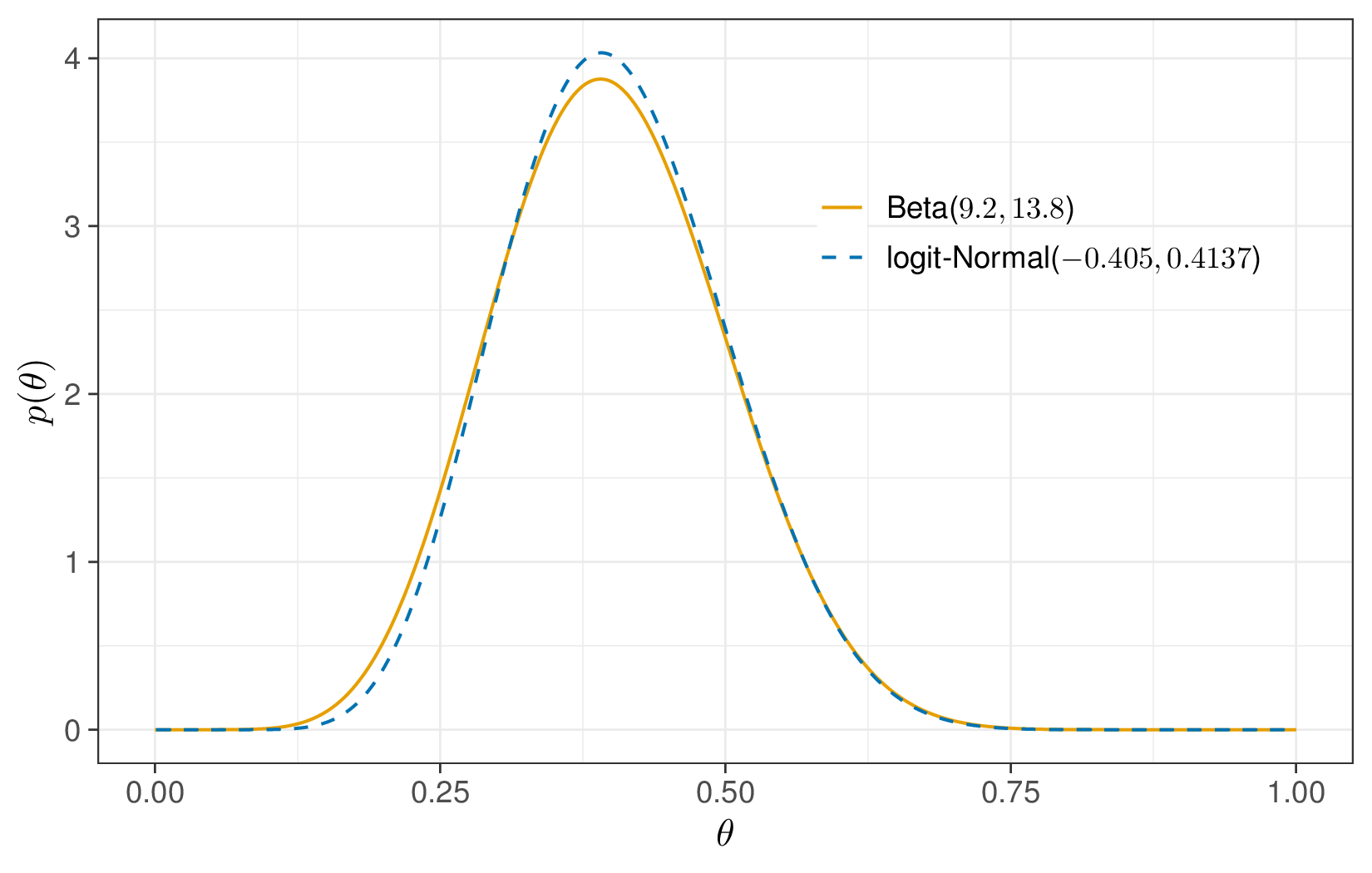
We can use trial-and-error or some simple algebra to derive values for \((m,s)\) so that the resulting distribution effectively matches the available information; for instance, setting \[\begin{eqnarray*} m &=& \text{logit}(\mu)\\ &=&\log\left(\frac{0.4}{1-0.4}\right)=-0.405 \end{eqnarray*}\] and \[\begin{eqnarray*} s &=& \frac{\text{logit}(\mu+2\sigma)-\text{logit}(\mu)}{z_{0.05}}\\ &=& \frac{\text{logit}(0.6)-\text{logit}(0.4)}{1.96} = 0.4137, \end{eqnarray*}\] where \(z_{0.975}\) is the point in a standard Normal distribution leaving 0.975 to its left4, effectively implies a distribution that, when rescaled to the natural \([0;1]\) range is, for all intents and purposes, identical with the \(\text{Beta}(9.2,13.8)\) prior discussed above (see Figure 1.11). Thus, \[\phi \sim \text{Normal}(-0.405, 0.4137) \Rightarrow \text{logit}^{-1}(\phi)=\frac{\exp(\phi)}{1+\exp(\phi)}=\theta \approx \text{Beta}(9.2,13.8)\] and we can use either distributional choices (a Normal on the logit scale, or a Beta on the natural scale) to encode the available prior information.
We can actually determine the analytic form of the implied distribution for \(\theta\), starting from modelling \(\phi=\text{logit}(\theta) \sim \text{Normal}(\mu,\sigma)\), by using a mathematical process, often described as “change of support variable” rule.
In general, if \(x \sim p_X(x)\) and \(y=f(x)\), which obviously implies that \(x=f^{-1}(y)\), then we can derive the distribution on the scale of \(y\) as \[ \begin{aligned}[b] p_{Y} (y) &= p_{X} (x) \left\lvert \frac{\partial f^{-1}(y)}{\partial y} \right\rvert\\ & = p_{X} \left(f^{-1}(y)\right) \left\lvert \frac{\partial f^{-1}(y)}{\partial y} \right\rvert, \end{aligned} \tag{1.14}\] where in general the notation \(\partial f(x) / \partial x\) indicates the first derivative of a function \(f(\cdot)\) with respect to the variable \(x\).
In the specific case discussed above, we have \(\phi \sim \text{Normal}(\mu,\sigma)\) for set values \(\mu=-0.405\) and \(\sigma=0.4137\) and \[\displaystyle \theta=f(\phi)=\frac{\exp(\phi)}{1+\exp(\phi)},\] which implies that \[ \phi = f^{-1}(\theta) = \log\left(\frac{\theta}{1-\theta}\right) = \log(\theta) - \log(1-\theta) \] and thus \[ \begin{aligned} \left\lvert\frac{\partial f^{-1}(\theta)}{\partial \theta}\right\rvert & = \left\lvert\frac{\partial \log(\theta) - \log(1-\theta)}{\partial \theta}\right\rvert \\ & = \left\lvert\frac{1}{\theta} + \frac{1}{1-\theta}\right\rvert = \left\lvert\frac{1}{\theta (1-\theta)}\right\rvert. \end{aligned} \] Applying Equation 1.14, we then get \[ \begin{aligned} p_{\theta}(\theta) & = p_{\phi}(f^{-1}(\theta))\left\lvert\frac{1}{\theta (1-\theta)}\right\rvert \\ &= \underbrace{\frac{1}{\sqrt{2\pi}\sigma}\exp\left(-\frac{1}{2}\frac{\left(\text{logit}(\theta) - \mu\right)^2}{\sigma^2}\right)}_{\text{Normal density computed at } \phi=\text{logit}(\theta)} \left\lvert\frac{1}{\theta (1-\theta)}\right\rvert, \end{aligned} \tag{1.15}\] which we write compactly as \(\theta\sim \text{logit-Normal}(\mu,\sigma)\).
We can code this computation up in a small R function
dlogitnorm=function(x,mu,sigma) {
  dnorm(log(x/(1-x)),mu,sigma)*abs(1/(x*(1-x)))
}
that we can use to determine the value of the logit-Normal density for any input x \(\in[0;1]\). Notice that, consistently with Equation 1.15, in the function dlogitnorm() the argument x is used to compute the Normal density at its logit, through the built-in R function dnorm(), whose first argument is transformed to log(x/(1-x)).
As an example, we can check that running in R the following commands
dlogitnorm(0.4,-0.405,0.413)[1] 4.024839dbeta(0.4,9.2,13.8)[1] 3.86089would return near identical values for the density computed at \(\theta=0.4\) for the two models.
More specifically, we can use the custom and built-in functions dlogitnorm() and dbeta() to compute the densities for a grid of \(\theta\) values in \([0;1]\) and then visualise the two resulting distributions, as in Figure 1.12. These are effectively identical (which is obviously aligned with the graph based on the histogram of Figure 1.11).
One consequence of working within a Bayesian environment is that we can use the prior distribution (which describes our current level of uncertainty on the model inputs, i.e. the parameters) to formally propagate onto the model outcomes, i.e. potentially observable data.
This is relevant, perhaps, at the stage of planning for a new study, when we make assumptions about the alleged DGP and the current state of science on its features to determine what we may be reasonably expect to observe if we managed to actually collect relevant data. In a Bayesian context, this effectively amount to estimating the (prior) predictive distribution (see Equation 1.7).
Example 1.5. Drug (continued): forward sampling. Consider again the situation described in Example 1.4; we have not obtained any data on actual patients taking the drug, yet; however, we can think of a suitable model to represent the sampling variability that the data would be subject to, if we were able to collect them.
For example, it may be reasonable to consider a possible study in which we observe \(n=20\) individuals suffering of back pain to whom we give the drug (the sample size \(n=20\) is totally arbitrary here and we could, in principle, select any number we can afford to recruit).
Assuming that the main outcome is \(y\), the total number of individuals who, upon taking the drug are relieved from the pain, we can use a Binomial distribution to model the sampling variability. This is defined by the probability distribution \[p(y\mid\theta) = \left( \begin{array}{c}n\\y\end{array} \right) \theta^y \; (1-\theta)^{n -y}. \tag{1.16}\]
Starting from the Monte Carlo sample of values from the prior \(p(\theta)\), which we have obtained in Example 1.4, we can now simulate nsim hypothetical, or “virtual” trials, by sampling y from its distribution and propagating “forward” the uncertainty over theta.
# Simulates from the (prior) predictive distribution of 'y'
y=rbinom(n=nsim,size=20,prob=theta)
(the parameters of the R function rbinom() are the number of simulations n, the sample size for each experiment, size and the probability of success, prob). Again, the actual number of simulations is entirely arbitrary; we may choose nsim=1000, just to fix the ideas.
This process basically “mixes up” the uncertainty in theta (as expressed by the simulations generated above) with the variability inherent to the sampling process for possible values of y, generated by the use of the function rbinom(). We can also record, for each simulated trial (i.e. each row of the vector y), whether the value drawn is greater than a specific threshold (say, 14 successes) in the variable P.crit.
P.crit=(y>=15)(note that we can define the “strictly greater than 14” condition as either y>14 or y>=15).
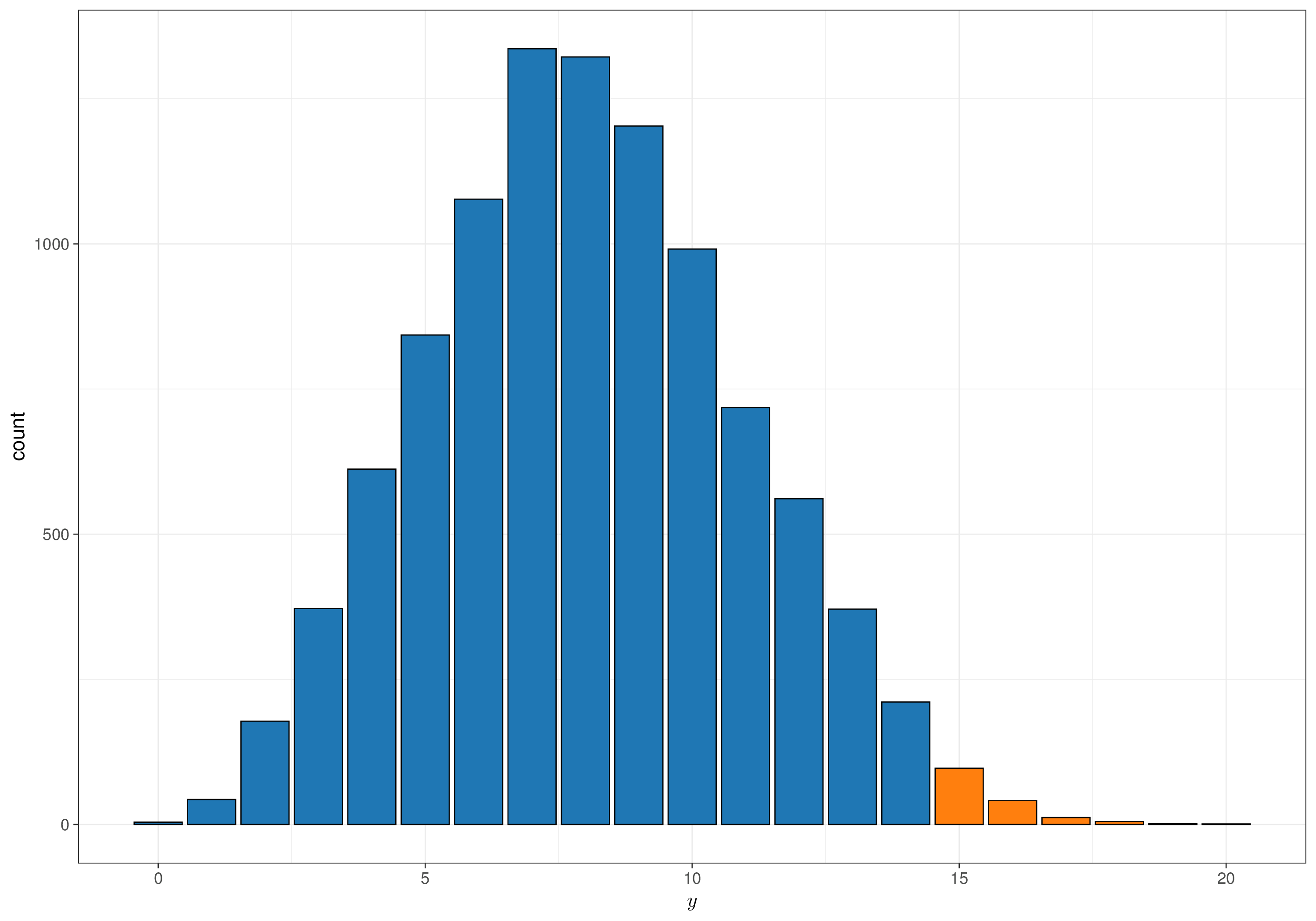
The resulting predictive distribution for \(y\) can be visualised as in Figure 1.13. The bars in lighter colouring indicate exceedance of the threshold, set at 15 or more successes – this may be derived by clinical or economic considerations (e.g. the trial would actually make sense if at least 15 individuals out of 20 benefitted from the treatment).
We can also use bmhe::stats() to give us a numerical summary of the distributions for y, P.crit and theta.
# Binds the vectors 'P.crit', 'y' and 'theta' into columns of a matrix
sims = cbind(P.crit,y,theta)
# Runs bmhe::stats to summarise the simulations
bmhe::stats(sims)
mean sd 2.5% median 97.5%
P.crit 0.0158000 0.1247073 0.0000000 0.0000000 0.000000
y 8.0175000 2.9632873 3.0000000 8.0000000 14.000000
theta 0.4018231 0.1002008 0.2172574 0.3984317 0.603672If we were actually conducting a trial, we would be expecting to observe an average of around 8 patients cured by the drug. It is unlikely that we would see a much bigger result, say above 14, which is the 97.5%-quantile of the distribution for \(y\). Consequently, the value for \(P_{crit}\) is, on average, very small (as apparent from Figure 1.13 too).
Obviously, the distribution of \(\theta\) is the same as in the prior – there is nothing in our set up with which to update it (i.e. we have not yet observed any data) and so our uncertainty about \(\theta\) cannot be updated, just yet.
In this chapter we have introduced the philosophical underpinning of Bayesian reasoning and have started to explore how Bayesian computation can include contextual information into the inference. We have started to discuss the mapping of background knowledge and information into a suitable prior distribution and use the process of forward sampling to propagate uncertainty to the model.
In the next chapter, we will look into using observed data to update the current uncertainty over unobserved and unobservable quantities. We will discuss more specifically different ways of defining the prior distributions and explore the basics of Bayesian computation, specifically in terms of Markov Chain Monte Carlo algorithms.
Interestingly, when Fisher joined University College London in 1933, a special chair as “Galton Professor of Eugenics” was created in the Department of Eugenics, so as to avoid him being in the then Department of Applied Statistics, which was led by Egon Pearson.↩︎
The author proudly acknowledges his very pedantic nature, nonetheless.↩︎
This is a luxury we can now enjoy, given that computing power is essentially very cheap. Before the advent of widely available personal computers in the 1980s and 1990s, especially, the “I can’t be bothered to do this integral” consideration was much less of an option…↩︎
This result derives from basic standard Normal theory and assuming that the interval \([\text{logit}(\mu-2\sigma);\text{logit}(\mu+2\sigma)]\) covers 95% of the entire probability mass. See also Example 9.2 for another example of this type of computation.↩︎