| Non smokers | Smokers | Total | ||||
|---|---|---|---|---|---|---|
| Success | Failure | Success | Failure | Success | Failure | |
| Treatment | 135 | 15 | 45 | 45 | 180 | 60 |
| Placebo | 50 | 50 | 6 | 54 | 56 | 104 |
| Total | 185 | 65 | 51 | 99 | 236 | 164 |
11 Population adjustment
11.1 Introduction
The methods described in Chapters 6 and 7 represent a progressive expansion from aggregated level summaries of a single pairwise comparison to the synthesis of an entire network of trials involving multiple treatments, simultaneously. Despite their differences in scope, these two frameworks share a common and consequential assumption, i.e. that the patient populations enrolled across the relevant studies are sufficiently exchangeable (see Section 6.2.4) and thus that pooling their results, whether directly or through a common comparator, yields estimates that are meaningful for the decision at hand.
However, when this is not tenable, naive pooling introduces bias into the indirect comparison, regardless of whether pairwise or network-based. This matters because, almost invariably, RCTs are designed with eligibility criteria that may differ substantially from one another and from the broader population of patients who will ultimately be treated, if the intervention is recommended. The network of evidence assembled through systematic literature review is therefore almost certain to comprise trials whose populations are heterogeneous in ways that matter for the estimated treatment effects.
In the case of fully available individual-level data, the wider biostatistics and causal inference literature has produced tools to deal with imbalance, e.g. using regression-based approaches such as propensity score (Rosenbaum and Rubin, 1983, 1984), as well as pure weighting-based tools, such as inverse probability weighting (Robins et al., 2000).
However, the structure of the data typically available for HTA submission exacerbates the problems even further: this is because while a sponsor may have direct access to the ILD from their own pivotal trial, the evidence on competing treatments exists, in the vast majority of cases, only in published aggregate form, typically consisting of average treatment effects and summary patient characteristics. This results in a structurally asymmetric evidence base: potentially rich, individual-level information on one arm of the comparison and only summary statistics on the other.
This asymmetry is precisely what creates both the motivation and the methodological challenge for the techniques we consider in this chapter, collectively referred to as population adjustment methods. The core objective of population adjustment is to produce estimates of relative treatment effect that are valid for a specific, well-defined target population, which is typically the population of patients for whom the healthcare decision is being made, rather than for the heterogeneous mix of trial populations from which the evidence happens to have been drawn, as described graphically in Figure 11.1.
Here, we consider an “anchored” comparison, where two active interventions (B and C) are separately compared to a common comparator (A). In the standard NMA framework of Chapter 7, we gain power by borrowing strength across the entire network of studies, under the key assumption that relative treatment effects are “consistent” (Dias et al., 2013, 2018), i.e. the effect of a B versus C, whether estimated directly or inferred through the common comparator A, is the same across all study populations in the network.
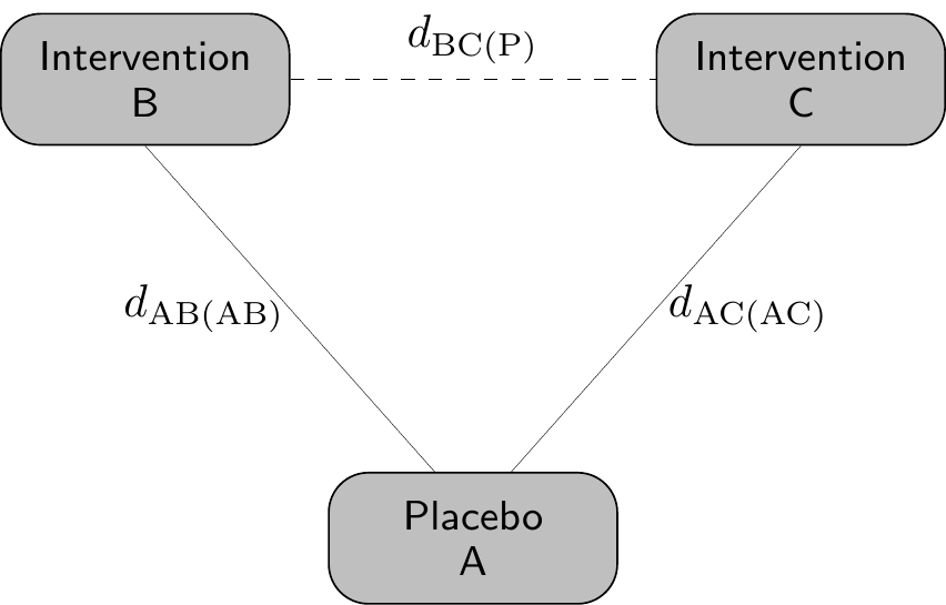
Mathematically and with respect to Figure 11.1, this implies \[ d_{\text{BC(P)}} = d_{\text{AC(AC)}} - d_{\text{AB(AB)}}, \tag{11.1}\] i.e. that the estimate for the effect of B vs C in the target population P can be obtained as the difference between the estimated effect of A vs C in the AC population and the estimated effect of A vs B in the AB population. In other words, under consistency, we can anchor the effect of the two treatments over the common comparator (placebo, in this case) and then by difference obtain the indirect treatment effect.
Of course, in reality, it is very possible that the two underlying populations AB and AC are fundamentally different, e.g. in terms of inclusion/exclusion criteria, or simply in terms of the distribution of the background characteristics (age, gender mix, co-morbidities, etc.), thus violating consistency. In addition, in Equation 11.1, the target population P is implicitly defined as a mixture of the original AB and AC populations, which again may not be a reasonable or helpful assumption in the HTA context.
To overcome these fundamental issues, the main idea of population adjustment is then to somehow rebalance the underlying characteristics of the populations in which the studies have been conducted, so that the resulting estimates of relative treatment effect are valid for a well-defined target population, rather than reflecting the potentially biased mix of trial populations from which the evidence was drawn.
11.2 Effect modifiers and collapsibility
One of the compounding issues in a general NMA framework such as that described in Figure 11.1 is that the unbalance in the background characteristics is generated by the presence of effect modifiers, as well as prognostic factors – see among others Phillippo et al. (2025a) and Phillippo et al. (2025b) for more details.
Prognostic factors are covariates that affect absolute outcomes, regardless of treatment. Typically, these are balanced in a RCT, which means that they pose no concerns in terms of NMA and indirect comparisons.
Conversely, effect modifiers are defined as covariates that do affect the treatment and thus impact on the estimators for the relative effects, e.g. \(\hat{d}_{\text{AC(AC)}}\) or \(\hat{d}_{\text{AB(AB)}}\). This means that relative effects obtained from different populations may not be the same and thus, if there is imbalance in the effect modifiers, then \[ \hat{d}_{\text{AC(AC)}} - \hat{d}_{\text{AB(AB)}} \neq \hat{d}_{\text{AC(P)}} - \hat{d}_{\text{AB(P)}}, \] which in turns implies that we cannot “transport” the indirect treatment effect to the target population P.
Perhaps even more importantly, the scale in which the analysis is performed may also lead to problematic results in terms of comparisons across different population – we explore these issues in Example 11.1.
Example 11.1. Effect modifiers and collapsibility. Consider the hypothetical (and, as usual, ridiculously simplified!) situation described by Table 11.1.
In this study, smoking status is a prognostic factor because overall response rates differ between smokers and non-smokers, regardless of treatment: \[ \Pr(\text{Success}\mid\text{Non-smokers})=\frac{185}{250}=0.74 \quad \text{and} \quad \Pr(\text{Success}\mid\text{Smokers})=\frac{51}{150}=0.34 \] and thus smoking status predicts the outcome.
Moreover, treatment is evenly distributed across the two strata of the smoking status variable: \[ \Pr(\text{Treatment}\mid\text{Non-smokers})=\frac{150}{250} = \Pr(\text{Treatment}\mid\text{Smokers})=\frac{90}{150}=0.6. \] Consequently, smoking is not a confounder and, in addition, for the purposes of this silly example, we assume that there are no other unobserved or unobservable confounder either.
Now, if we consider as a measure of the treatment effect the risk difference \[ \text{RD}= \Pr(\text{Success}\mid \text{Treatment})-\Pr(\text{Success}\mid \text{Placebo}) \] and compute it in the strata (NS and S for Non-smokers and Smokers, respectively), we get \[ \text{RD}_{\text{NS}} = \frac{135}{150}-\frac{50}{100}=0.4, \quad \text{and} \quad \text{RD}_{\text{S}} = \frac{45}{90}-\frac{6}{60}=0.4 \] and so the treatment does not have a differential effect across different levels of smoking, which is thus not an effect modifier.
Similarly, if we use the OR as a measure of treatment effect (and recalling Equation 6.8), we get that \[ \text{OR}_{\text{NS}}=\left. \frac{135/150}{15/150}\middle / \frac{50/100}{50/100} \right. = 9 \quad \text{and} \quad \text{OR}_{\text{S}}=\left. \frac{45/90}{45/90}\middle / \frac{6/60}{54/60} \right. = 9, \] so that, again, the effect of the treatment does not vary across strata defined by smoking, which again is not an effect modifier.
Conversely, when considering the risk ratio \[ \text{RR}=\left. \Pr(\text{Success}\mid\text{Treatment}) \middle / \Pr(\text{Success}\mid\text{Placebo}) \right. \] we have in the two subgroups \[ \text{RR}_{\text{NS}}=\left. \frac{135}{150}\middle / \frac{50}{100} \right. = 1.8 \neq \text{RR}_{\text{S}}=\left. \frac{45}{90}\middle / \frac{6}{60} \right. = 5, \] indicating that, on this scale, smoking is indeed an effect modifier.
The interpretation across different scales becomes in fact more complex, because even in situations seemingly identical we may get further differences. For instance, for both the RD and the OR, the data in Table 11.1 suggest treatment effect homogeneity (i.e. no confounding, as well as perfect balance and no effect modification).
In the case of the RD, the crude overall effect \[ \text{RD}_{\text{crude}} = \frac{180}{240}-\frac{56}{160}=0.4 \] coincides with the weighted average of the stratum-specific ones \[ \begin{aligned} \text{RD}_{\text{weighted}}& =w_{\text{NS}} \text{RD}_{\text{NS}} + w_{\text{S}}\text{RD}_{\text{S}} \\ & = \frac{250}{400} 0.4 + \frac{150}{400} 0.4 = 0.4, \end{aligned} \] where \(w_{\text{NS}}\) and \(w_{\text{S}}\) are the proportion of the total sample size in each of the strata. This property is referred to as collapsibility (Greenland et al., 1999) and thus we say that the RD is collapsible.
On the other hand, collapsibility does not hold for the OR, because the crude value is \[ \text{OR}_{\text{crude}}=\left. \frac{180/240}{60/240}\middle / \frac{56/160}{104/160} \right. = 5.6, \] which differs from the weighted average among the strata \[ \begin{aligned} \text{OR}_{\text{weighted}} & = \exp\left( w_{\text{NS}}\log(\text{OR}_{\text{NS}}) + w_{\text{S}}\log(\text{OR}_{\text{S}}) \right) \\ & = \exp\left(\frac{250}{400} \log(9) + \frac{150}{400} \log(9)\right) = 9 \end{aligned} \] – this quantity averages the stratum-specific effects on the scale of the linear predictor (i.e. log OR rather than directly OR). The crude estimates identify the population marginal effects, while the weighted estimates are the population conditional effects.
In the absence of effect modification, for non-collapsible measures the direction of the treatment effect aligns, but the magnitude generally varies when considering the population average marginal vs conditional effects. More problematically, when there is effect modification, the rank ordering of the treatments may even flip.
Interestingly, an effect modifier may still be collapsible. For instance, even if smoking were an effect modifier for the RD, the crude and weighted estimates would still coincide. This is due to the mathematical form of the estimand, which in the case of the RD is linear. It is for this reason that measures such as the OR or the HR are non-collapsible (see also the discussion in Note 8.5, in Section 8.4.6).
Similarly, effect modification is not a key factor for an RR to be collapsible: in fact, the requirements are that a covariate is not a confounder and that the baseline risk is balanced across its strata. In the specific context of the data in Table 11.1, if we had that
\[
\Pr(\text{Treatment}\mid\text{Non-smokers})=\Pr(\text{Treatment}\mid\text{Smokers})
\] and \[
\Pr(\text{Success} \mid \text{Placebo, Non-smoker}) = \Pr(\text{Success} \mid \text{Placebo, Smoker}).
\] then even if smoking were an effect modifier for the RR, this would still be collapsible.
In the next sections, we consider specific methods that are prevalent in the HTA context that are used to perform population adjustment.
11.3 Methods for population adjustment
Historically, the two most widely used population adjustment methods in HTA practice are Matching-Adjusted Indirect Comparison (MAIC, Signorovitch et al., 2010, 2012) and Simulated Treatment Comparison (STC, Caro and Ishak, 2010; Ishak et al., 2015).
MAIC is a propensity score-like reweighting approach that adjusts the individual-level data from one trial (typically the sponsor’s study) to match the aggregate summary statistics reported from the comparator trial. Specifically, it assigns weights to individuals in the ILD trial such that the weighted means of the observed covariates align with the published means from the aggregate data study. The weighted outcomes are then used to estimate the treatment effect in the reweighted (now “matched”) population.
Conversely, STC is a regression-based method that models the relationship between covariates and outcomes in the ILD trial and then uses this fitted model to predict the expected outcomes, had the ILD trial enrolled a population with the covariate distribution of the comparator study.
Despite their widespread adoption (particularly for MAIC), both methods have well documented limitations. Similarly to other weighting procedures, MAIC can suffer from extreme or unstable weights, when covariate overlap between the trials is poor, leading to high variance and potentially unreliable estimates. This problem worsens as the number of adjustment covariates increases, relative to the effective sample size1 (Phillippo et al., 2016, 2018). As for STC, due to its nature as a regression-based method, it avoids the weighting instability of MAIC. However, it is affected by other important limitations: its typical implementation directly targets conditional treatment effects on the scale of the outcome model, rather than marginal effects. As discussed above, this can lead to bias when the outcome model is non-linear or when non-collapsible effect measures such as ORs or HRs are used (Remiro Azócar et al., 2021).
In addition, both standard MAIC and STC crucially target the population of the comparator trial, which may not be the one relevant to the decision-maker, while also failing to naturally accommodate network structures involving more than two treatments without performing multiple pairwise adjustments and then pooling them in a secondary meta-analysis (thus introducing further, most likely untestable, assumptions).
To overcome these problems, research in the area of population adjustment has been particularly active in the past few years, producing important contributions. Among these, notable examples are multilevel network meta-regression (ML-NMR, Phillippo et al., 2020, 2025a), which extends population adjustment to arbitrary network structures and allows inference in any specified target population; and outcome regression standardisation, based on g-computation (Remiro Azócar et al., 2022) or marginalisation via multiple imputation (MIM, Remiro Azócar et al., 2024), which address the marginalisation problem in STC by constructing marginal effect estimates through imputation of missing covariate data in the aggregate trials.
Interestingly, these methods have a very strong Bayesian flavour, as well as marked computational complexity, which is however limited by the availability of suitable R packages to perform the underlying analyses – respectively multinma (Phillippo, 2024) and outstandR (Green et al., 2026). In the next sections we present the general modelling structure, highlighting relevant issues in terms of the target estimands and then review the basic assumptions and computational working of the two methods.
11.3.1 Multilevel Network Meta-Regression
The main idea underlying ML-NMR is to build a model capable to connect the two modules, one for the ILD and the other for the ALD evidence, so as to ensure that population-level parameters are derived consistently, avoiding aggregation bias and accounting for non-collapsibility, all well established problems in the wider evidence synthesis literature (Sutton et al., 2008; Saramago et al., 2012; Donegan et al., 2013).
The general individual-level data modelling structure proceeds as follows. We typically have data on individuals \(i=1,\ldots,n_{st}\) under each treatment arm \(t=1,\ldots,T\) in study \(s=1,\ldots,S\). Each study \(s\) is typically conducted in a specific population, which may differ from the others in terms of eligibility criteria, demographic characteristics and the distribution of prognostic factors and effect modifiers. The target population P may be one of these, or an entirely different one.
Almost invariably, in the notation of Figure 11.1, at least one study involves a comparison between interventions A vs B, where \(t=\text{A}\) is some kind of placebo or standard of care and \(t=\text{B}\) is the active intervention, to be contrasted with another active intervention C, considered in other studies. The data are modelled as \[ y_{ist} \sim p\left(y_{ist} \mid \boldsymbol{\theta}_{ist}\right), \] with parameters \(\boldsymbol{\theta}_{ist}=\left(\mu_{ist},\boldsymbol{\alpha}_{ist}\right)\), where \(\mu_{ist}\) is the individual mean outcome (which typically depends on some relevant covariates) and \(\boldsymbol{\alpha}_{ist}\) are a set of possible ancillary parameters (e.g. standard deviations, scales, shape parameters, etc.); the ancillary parameters may or may not be made to depend on the covariates and in fact may or may not be present, depending on the functional form of the sampling distribution \(p(\cdot)\). This is similar to the description given in Section 5.2.2 and Section 8.3.3.
We then construct a (generalised) linear predictor \[ g\left(\mu_{ist}\right) = \eta_{st}(\boldsymbol{x}_{ist}) = \beta_{0s} + \boldsymbol{x}_{ist}^\top(\boldsymbol{\beta}_1 + \boldsymbol{\beta}_{2t}) + \gamma_t \tag{11.2}\] where: \(g(\cdot)\) is the link function; \(\beta_{0s}\) is the study-specific intercept, representing baseline risk or outcome level in study \(s\) (stratified to preserve randomisation); \(\boldsymbol{x}_{ist}\) are the observed covariates for individual \(i\) in study \(s\) on treatment \(t\); \(\boldsymbol{\beta}_1\) identifies the prognostic effects (covariates that affect absolute outcomes but not treatment effects); \(\boldsymbol{\beta}_{2t}\) are treatment-covariate interaction terms capturing effect modification (with \(\boldsymbol{\beta}_{2\text{A}}=\boldsymbol{0}\) for the reference treatment A); and \(\gamma_t\) is an individual-level treatment effect for an individual with \(\boldsymbol{x}_{ist}=\boldsymbol{0}\), with \(\gamma_\text{A}=0\).
As for studies where only aggregated summaries are published, ML-NMR constructs the likelihood by integrating Equation 11.2 over the joint distribution of covariates within each study arm. For each aggregated outcome \(y_{\scriptstyle\bullet st}\) observed in study \(s\) and for arm \(t\), the model is specified as: \[ \begin{aligned} y_{\scriptstyle\bullet st} &\sim p(y_{\scriptstyle\bullet st} \mid \boldsymbol{\theta}_{\scriptstyle\bullet st}) \\ \mu_{\scriptstyle\bullet st} &= \int_\mathcal{X} g^{-1}( \eta_{st}(\boldsymbol{x}) ) f_{st}(\boldsymbol{x}) \, d\boldsymbol{x}, \end{aligned} \tag{11.3}\] where \(\boldsymbol{\theta}_{\scriptstyle\bullet st} = (\mu_{\scriptstyle\bullet st}[, \boldsymbol{\alpha}_{\scriptstyle\bullet st}])\) – again, ancillary parameters may or may not exist, depending on the distributional form chosen for the aggregated level data. In Equation 11.3, \(f_{st}(\boldsymbol{x})\) denotes the joint covariate distribution in that study arm and \(\mathcal{X}\) is its possible range.
The model is completed by specifying suitable prior distributions for the parameters – in the most basic structure implemented in the R package multinma, \(\beta_{0s} \sim \text{Normal}(0,\text{sd}=100)\) and \(\gamma_t,\boldsymbol{\beta}_1,\boldsymbol{\beta}_{2t} \stackrel{iid}{\sim} \text{Normal}(0,\text{sd}=10)\). The models are constructed in Stan using a process akin to that shown for survHEhmc and survextrap in Sections 8.4 and 8.5.1, respectively.
There are several advantages to using a Bayesian framework, even in the face of the underlying computational complexity. Firstly, using a Bayesian approach allows us to propagate fully the uncertainty in the marginalisation integral, as part of the posterior sampling. In addition, as the model naturally assumes some forms of (conditional) exchangeability in the ILD and ALD components, the Bayesian framework makes it easier to, at least conceptually, handle the underlying correlation across the modules.
On the other hand, the need to evaluate the marginalisation integral (once at each MCMC iteration) does impose a computational burden on this modelling structure. To limit this, ML-NMR uses numerical approximation based on Quasi-Monte Carlo (QMC) integration. This is a form of approximation for multidimensional integrals, obtained by averaging a function over a carefully chosen deterministic sequence of points, rather than exploring the full space randomly.
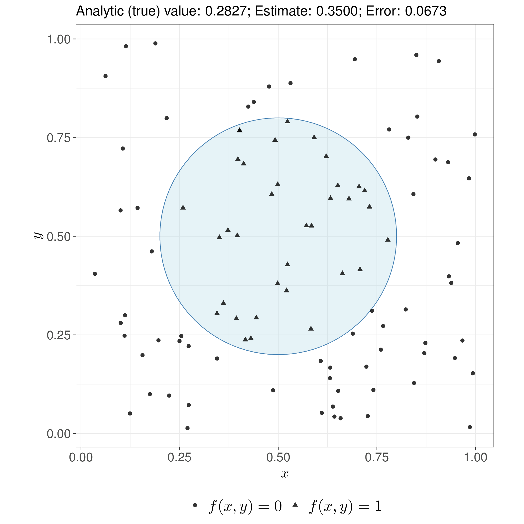
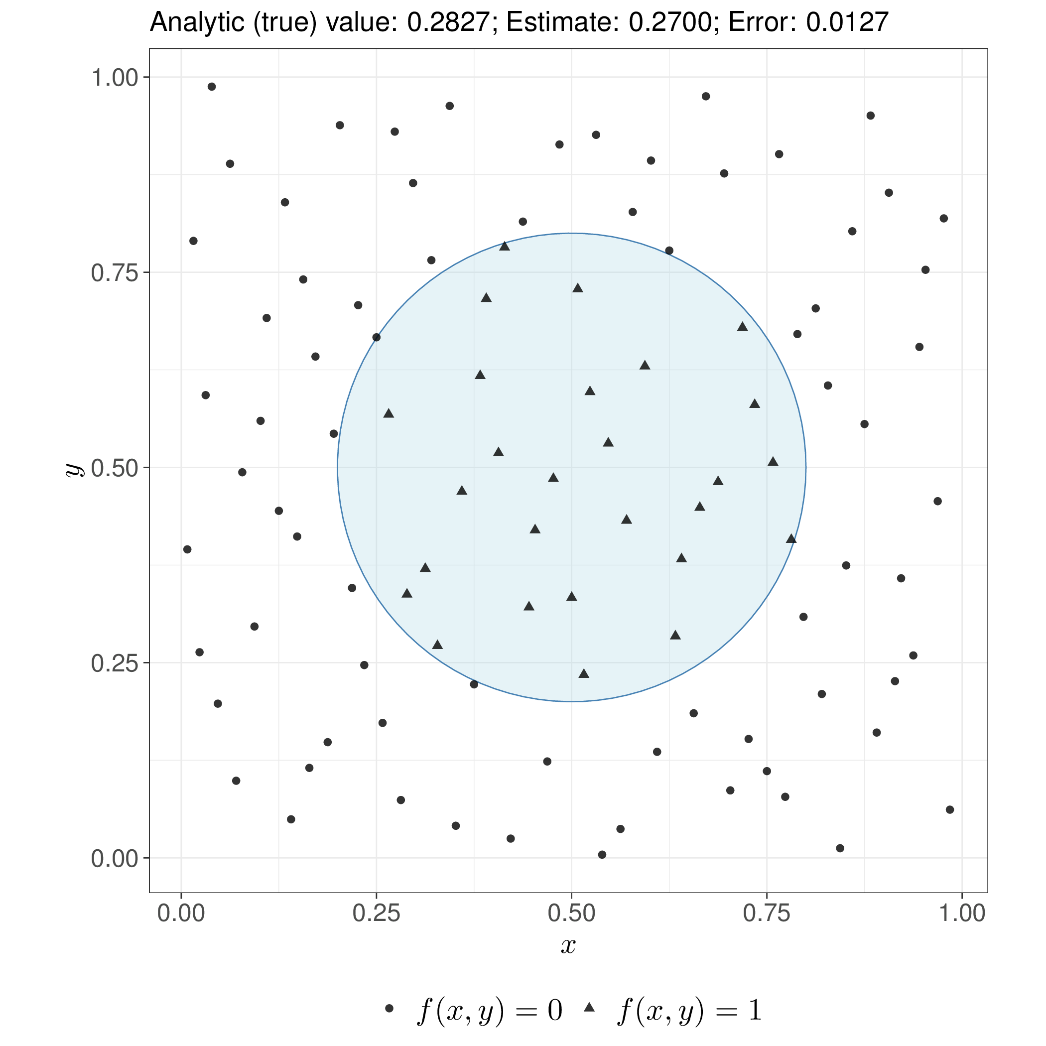
Unlike standard pseudo-random numbers-based Monte Carlo (see Section 1.2.4), QMC exploits numerical sequences designed to fill the target space more uniformly, with fewer gaps and “clumps”. For smooth functions, this can achieve convergence rates close to \(\mathcal{O}(n^{-1})\) rather than Monte Carlo’s \(\mathcal{O}(n^{-1/2})\), although the advantage diminishes in very high dimensions or for non-smooth integrands – a simplified example of this comparison is shown in Figure 11.2.
The specification in Equation 11.3 assumes that the aggregated level sampling distribution has a tractable, known form, which holds for standard outcome types (Normal, Binomial, Poisson, Multinomial) but not universally. For outcomes such as survival times where no natural aggregate distribution exists, ML-NMR can instead work directly with the likelihood contributions from each data level, avoiding the need for an explicit aggregated distribution, thus enabling broader applicability including time-to-event models (Phillippo et al., 2024).
The crucial advantage of ML-NMR for healthcare decision-making is its capacity to produce treatment effect estimates in any specified target population P, not merely in the populations of the observed studies – that is, provided we can reliably estimate the covariate distributions!
Using again the slightly more verbose notation presented in Figure 11.1, for a target population with joint covariate distribution \(f_{\text{(P)}}(\boldsymbol{x})\), the population-average conditional treatment effect between treatments B and C is derived from Equation 11.2 as \[ \begin{aligned} d_{\text{BC(P)}} &= \int_\mathcal{X} \left( \eta_{\text{B(P)}}(\boldsymbol{x}) - \eta_{\text{C(P)}}(\boldsymbol{x}) \right) f_{\text{(P)}}(\boldsymbol{x}) \, d\boldsymbol{x} \\ &= \bar{\boldsymbol{x}}_{\text{(P)}}^\top (\boldsymbol{\beta}_{2\text{B}} - \boldsymbol{\beta}_{2\text{C}}) + \gamma_\text{B} - \gamma_\text{C}, \end{aligned} \tag{11.4}\] where \(\mathcal{X}\) is the support of the covariates and the closed-form expression in terms of mean covariate values \(\bar{\boldsymbol{x}}_{\text{(P)}}\) in population P derives from the linearity of the treatment contrast on the linear predictor scale. This estimator is in the same spirit of Equation 5.9, as discussed in Section 5.2.2 and it represents the average individual-level treatment effect when the entire population P is shifted from treatment C to treatment B.
Notably, computing the population-average conditional treatment effect requires only the means of effect-modifying covariates in the target population: neither the full joint distribution nor information about baseline risk is needed for conditional effects.
However, as discussed in Note 6.1 in Section 6.2, economic models are based on absolute outcome predictions, rather than relative treatment effects. Thus, for a generic treatment \(t\), the target estimand in population P is \[ \bar{\mu}_{t\text{(P)}} = \int_\mathcal{X} g^{-1}\left( \eta_{t\text{(P)}}(\boldsymbol{x}) \right) f_{\text{(P)}}(\boldsymbol{x})d\boldsymbol{x}. \tag{11.5}\] Because the quantity inside the integral in Equation 11.5 depends on the typically highly non-linear function \(g(\cdot)\), in this case we do require the full joint covariate distribution \(f_{\text{(P)}}(\boldsymbol{x})\), which is rarely reported in a meaningful way, since published aggregate data studies typically provide only marginal summaries such as means, standard deviations or frequencies, for each covariate separately.
ML-NMR addresses this by reconstructing plausible joint distributions using copula methods (originally introduced by Sklar, 1959; but see also Joe, 2014 for a more recent detailed account), which combine the reported marginal summaries with assumed correlation structures and marginal distributional forms borrowed from the individual patient data studies (Phillippo et al., 2020).
Once absolute outcome predictions are available, population-average marginal treatment effects can also be estimated as \[ \delta_{\text{BC(P)}} = g\left(\bar{\mu}_{\text{B(P)}}\right) - g\left(\bar{\mu}_{\text{C(P)}}\right). \tag{11.6}\] These differ from the conditional effects in Equation 11.4 whenever the effect measure is non-collapsible (see Example 11.1) and quantify the change in the overall population event occurrence, when shifting from one treatment to another. Importantly, they can only be computed if the distribution \(f_{\text{(P)}}(\boldsymbol{x})\) is reliably estimated.
Evidence from simulation work indicates that ML-NMR estimates tend to be reasonably stable under mis-specification of the estimated covariate distribution, although models with substantial non-linearity or analyses targeting directly marginal rather than conditional estimands may exhibit greater sensitivity.
Example 11.2. Conditional vs marginal estimates. We return to the overly-simplistic case of Example 11.1. From Table 11.1, we can compute the distribution of the covariate \(x=\) Smoking status in the target population as \(f(\text{NS})=250/400=0.625\) and \(f(\text{S})=150/400=0.375\). The stratum-specific means (which in this case can be defined as probabilities) are \[ \mu_{\text{B}}(\text{NS})=\frac{135}{150}= 0.9 \quad \text{and} \quad \mu_{\text{A}}(\text{NS})=\frac{50}{100}= 0.5 \] and \[ \mu_{\text{B}}(\text{S})=\frac{45}{90}= 0.5 \quad \text{and} \quad \mu_{\text{A}}(\text{S})=\frac{6}{60}= 0.1, \] where A indicates the placebo and B indicates the treatment arms. Assuming \(g(\cdot)=\text{logit}(\cdot)\) and using these estimates, we can compute the average of Equation 11.4 as the discrete sum \[ \begin{aligned} d_{\text{BA}} & = \sum_x \left[\eta_{\text{B}}(x) - \eta_{\text{A}}(x)\right] f(x) \\ &= \left[\text{logit}\left( \mu_{\text{B}}(\text{NS}) \right) - \text{logit}\left( \mu_{\text{A}}(\text{NS}) \right)\right] f(\text{NS}) + \left[\text{logit}\left( \mu_{\text{B}}(\text{S}) \right) - \text{logit}\left( \mu_{\text{A}}(\text{S}) \right)\right] f(\text{S}) \\ &= \left( 2.1972 - 0 \right) 0.625 + \left( 0 + 2.1972 \right) 0.375 = 2.1972. \end{aligned} \]
Conversely, in line with Equation 11.5, the population-average marginal treatment effect is computed with respect to the example in Table 11.1 as \[ \bar{\mu}_{\text{B}} = \sum_{x}\mu_{\text{B}}(x)f(x) = 0.9 \times 0.625 + 0.5 \times 0.375 = 0.75 \] and \[ \bar{\mu}_{\text{A}} = \sum_{x}\mu_{\text{A}}(x)f(x) = 0.5 \times 0.625 + 0.1 \times 0.375 = 0.35 \] – note that these quantities coincide with the crude estimates from the “Total” part of Table 11.1. Using these, we can compute the discrete version of Equation 11.6 as \[ \begin{aligned} \delta_{\text{BA}} = g(\bar{\mu}_{\text{B}}) - g(\bar{\mu}_{\text{A}}) & = \text{logit}(\bar{\mu}_{\text{B}}) - \text{logit}(\bar{\mu}_{\text{A}}) \\ & = 1.0986 - (-0.619) \\ & = 1.7177 \end{aligned} \] Because of the non-collapsibility of the logit, we get that \(d_{\text{BA}}\neq \delta_{\text{BA}}\).
When few aggregate data studies are available for a particular treatment, insufficient information may exist to estimate the relevant treatment-covariate interaction terms, \(\boldsymbol{\beta}_{2t}\). This situation may require a “shared effect modifier” assumption, in which interactions are constrained to be constant across a treatment set (Phillippo et al., 2020). Such an assumption might be defensible when treatments share pharmacological class and mechanism of action, but is otherwise restrictive. Under this constraint, interaction effects can be borrowed from treatments with individual patient data or pooled across multiple aggregate data treatments.
In a minimal two-study comparison with aggregate data for only one treatment, this reduces ML-NMR to the same limitation as MAIC and STC: estimates are constrained to the aggregate study population. However, in networks of moderate size, the shared effect modifier assumption can often be tested by selectively relaxing constraints or avoided entirely given sufficient data (Phillippo et al., 2023). Furthermore, the fundamental assumption underlying all population adjustment, conditional constancy of relative effects, can be evaluated within the ML-NMR framework using standard network meta-analysis diagnostics for heterogeneity and inconsistency, as discussed in Chapter 7.
Worked examples using ML-NMR are shown in Phillippo et al. (2025a) and in the multinma website https://dmphillippo.github.io/multinma/.
11.3.2 Outcome regression standardisation using g-computation
Both MAIC and STC, as well as ML-NMR, fundamentally address the problem of transporting treatment effect estimates to a target population when covariate distributions differ across studies. However, as mentioned above, a distinct challenge arises in the context of outcome regression methods like STC: the standard implementation targets conditional treatment effects on the scale of the outcome model, rather than the marginal effects required for population-level decision-making in HTA (Remiro Azócar et al., 2021, 2022).
As discussed in Example 11.1, when the effect measure is non-collapsible, conditional and marginal effects diverge, even in the absence of treatment-covariate interactions. Standard STC methods that simply plug predicted outcomes into the regression model therefore produce biased estimates of the marginal treatment effect in the target population.
To overcome this issue, Remiro Azócar et al. (2022) propose using parametric g-computation (where “g” stands for “generalised”, as originally defined in Robins, 1986), a method borrowed from the causal inference literature, which predicts the natural-scale outcome under different treatment strategies by using a regression model and then averages those predictions over the covariate distribution in the population of interest, to obtain estimates for the relevant marginal effects. In a Bayesian context (and assuming the absence of unobserved confounding – see Daniels and Hogan, 2008), this essentially amounts to the discussion of Section 5.2.3 and the general model can be visualised as in Figure 11.3.
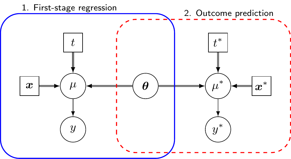
In the specific context of the HTA population adjustment case, we first fit an outcome regression model to the available individual patient data from the AB study, for instance using the same general structure as in Equation 11.2. This is indicated as “First-stage regression” in Figure 11.3. In a Bayesian context, we thus obtain \(L\) samples from the posterior distributions of the parameters \(\boldsymbol{\theta}\), including the regression coefficients \(\boldsymbol{\beta}\) (which capture treatment effects and covariate relationships) and any relevant ancillary parameters \(\boldsymbol{\alpha}\), such as variances or dispersion parameters.
We then use the published aggregate summaries from the AC study to reconstruct the joint covariate distribution \(f_{\text{AC}}(\boldsymbol{x})\). This typically involves fitting parametric distributions (e.g. multivariate Normal for continuous covariates, or Multinomial distributions for categorical variables), with the correlation structure borrowed from the individual patient data, if needed. Alternatively, we can rely on copula-based methods, similarly to ML-NMR. Either way, we can use this distribution to simulate a full vector of covariates \(\boldsymbol{x}^* \sim f_{\text{AC}}(\boldsymbol{x})\).
At this point, we can consider a sample of \(N^*\) synthetic individuals from the AC population with individual-level profiles \(\boldsymbol{x}^*_i\) and use the output from the first-stage regression \(\boldsymbol{\theta}\) to predict the outcome \(y^*\) that might be observed in the AC population, had those individuals be allocated to \(t^*\in \{A,B\}\). In particular, we consider a sample where the covariates profile is balanced (in fact, identical in the specification of Remiro Azócar et al., 2024) across the intervention arms, so that the treatment effect can be identified without further issues.
The two steps of model fitting and outcome prediction can be embedded in a single Bayesian modelling operation. For each synthetic individual \(i=1,\ldots,N^*\), we can draw \(l=1,\ldots,L\) samples from the predictive distribution \(y^{*{(l)}}_{it{^*}} \sim p\left(y_{i{t^*}} \mid \boldsymbol{\theta}^{(l)}, \boldsymbol{x}^*_i\right)\). Averaging these predicted outcomes across the \(N^*\) synthetic individuals gives us marginal outcome predictions \(\bar{y}_{t^*}^{(l)}\) from which we can compute a sample of \(L\) estimates of the marginal treatment effects such as the B vs A effect in the AC population, i.e. \[ \Delta^{(l)} = \bar{y}_{\text{B}}^{(l)} - \bar{y}_{\text{A}}^{(l)}, \] which can be used to provide summaries for the underlying distribution (e.g. mean and intervals).
The approach explicitly targets marginal estimands, ensuring compatibility in indirect comparisons when effect measures are non-collapsible and can extrapolate beyond observed covariate overlap, unlike propensity score methods such as MAIC.
On the other hand, parametric g-computation has some important limitations. First, the in its basic construction, it is restricted to pairwise indirect comparisons, similarly to the “vanilla” implementation of STC. While in principle the method could be extended to larger networks by performing multiple pairwise comparisons and synthesising the results, this requires additional assumptions and does not naturally leverage the full network structure in the way that ML-NMR does.
In addition, the validity of the marginal effect estimates depends critically on the correct specification of both the outcome regression model and the parametric distributions used to generate the synthetic covariate data. Mis-specification of either component can introduce bias and there is limited ability to check model fit in the aggregate data study, where individual-level observations are unavailable. This is particularly concerning when extrapolating to covariate regions poorly represented in the ILD.
Finally, the computational burden of running this approach can be substantial. The process requires generating a complete pseudo-ILD dataset and computing predictions for every synthetic individual at each iteration of the uncertainty quantification procedure. With typical choices of \(L \approx 4000\) posterior draws and \(N^* \approx 1000\) synthetic individuals, this results in millions of individual-level predictions.
The computational cost is further compounded when the outcome model is complex. For survival models with flexible baseline hazards (such as spline-based approaches), each prediction requires numerical integration to compute survival probabilities. For count or other generalised linear models with overdispersion, additional random draws are needed for dispersion parameters. When multiple treatments are being compared, the number of predictions scales linearly with the number of treatment arms.
11.3.3 Multiple imputation marginalisation
Multiple imputation marginalisation (MIM) addresses both the computational limitations and some conceptual gaps of standard parametric g-computation by embedding the outcome regression standardisation process within the established framework of multiple imputation (Remiro Azócar et al., 2024).
The first part of MIM is essentially identical to the process described in Figure 11.3, in which we generate \(L\) samples from the predictive distribution for the outcome \(y^*\) that might be observed in \(N^*\) synthetic individuals from the AC population, if they were allocated to treatments in \(t^*=\{A,B\}\) instead. However, to simplify the rest of the computation, MIM proceeds to “thin” the \(L\) simulations for \(\boldsymbol{\theta}\) to only consider a number \(M<<L\) – typically, \(M=20 \text{ to }50\) “imputations”, in missing data parlance (see Section 10.3.1).
These process basically amounts to create \(M\) “complete” versions of the full dataset that might be observed if a AB trial with \(N^*\) individuals were run in the AC population. In the analysis stage (depicted in Figure 11.4), each of these \(m=1,\ldots,M\) imputed datasets is analysed separately, by modelling the relationship between the predicted outcome \(y^{*(m)}\) and the treatment assignment \(t^*\), using a generalised linear regression such as \[ g\left(\eta^{(m)}_i\right) = \phi_0^{(m)} + \delta^{(m)}t^*_i, \tag{11.7}\] where \(\phi_0^{(m)}\) is the intercept and \(\delta^{(m)}\) is the relevant marginal treatment effect – again, because we are constructing the \(N^*\) individuals as perfectly balanced in terms of background characteristics, we do not need to control for the effect of \(\boldsymbol{x}^*\) in Equation 11.7.
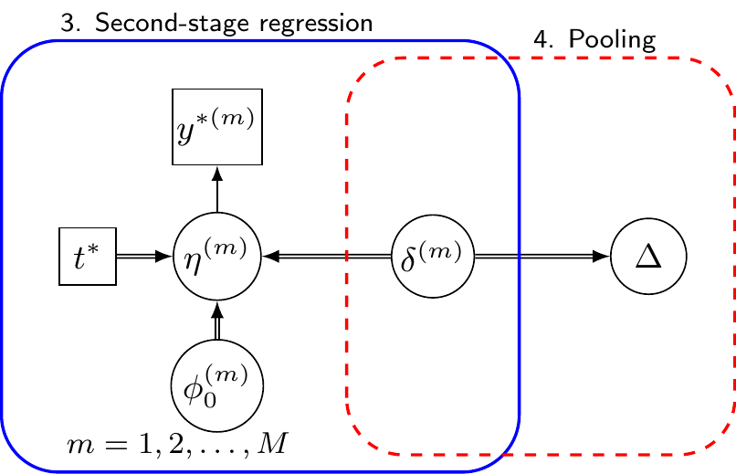
Again, within a full Bayesian setting, we can obtain \(R\) samples from the posterior distribution of the relevant parameter \(\delta^{(m)}\) – but this time the overall size \(M\times R\) allows for a much more feasible computation. Using these we can pool the point estimates for \(\delta^{(m)}\) and their resulting variances, e.g. using Rubin’s rule, to produce the pooled estimate of the treatment effect, accounting for both within-imputation uncertainty (how much predictions vary within one synthetic dataset) and between-imputation uncertainty (how much the \(M\) datasets differ from each other due to the random sampling of covariates).
The R package outstandR (Green et al., 2026) implements both maximum likelihood and Bayesian versions of MIM, along with standard outcome regression standardisation using g-computation and other population adjustment methods – some examples are presented in the package website https://statisticshealtheconomics.github.io/outstandR/.
In particular, the Bayesian formulation for MIM offers several advantages: it naturally handles uncertainty in regression parameters without bootstrap resampling, readily accommodates missing data in the ILD study itself through standard multiple imputation techniques and allows incorporation of prior information about model parameters or covariate distributions. The full posterior distribution provides a natural input for probabilistic sensitivity analysis in downstream economic models (see Section 4.3).
11.4 Further challenges
While population adjustment is gaining increasing popularity in the HTA context and the established methods described above are becoming more and more relevant and used in applied analyses, there are still numerous research questions unresolved and possible extensions to the existing methods.
Among these, Gao et al. (2025) discuss the further complexity generated by the presence of heterogeneous treatment effects, while Campbell et al. (2026) extend the general framework of ML-NMR to consider subgroup-level summary statistics that may be available in published studies and potentially highly informative.
11.5 Conclusions
In this chapter we have discussed the general framework underpinning the important problem of population adjustment. This is particularly key in HTA, because naive indirect comparison may very easily produce biased (and irrelevant!) estimates for the relevant treatment effect parameters, which would of course have dire consequences in terms of the meaningfulness of the economic evaluation.
We have presented recent development in statistical methodology, which are gaining substantial traction and becoming very popular in the HTA context. These have all a very strong Bayesian nature and thus fit nicely with the overall Bayesian decision-making process.
In the next chapter, we will present the most important features (both in terms of methodology and applications) of the important analysis of the value of information, a suite of tools that can be used to measure the economic value of additional information.
In the context of MAIC, the effective sample size quantifies the loss of information due to reweighting – essentially, how many “independent” observations remain after adjustment/matching.↩︎