7  Indirect treatment comparisons

7.1 Introduction

Evidence synthesis and meta-analysis (as presented in Chapter 6) are particularly efficient when we need to pool estimates of a common parameter across different studies. This is typical in much of clinical research, where often there is a number of studies on a common comparison of interest, e.g. treatment \(t=2\) against placebo \(t=1\).

In HTA, this setup is not ideal, however; this is because the actual comparison of interest for the economic model is almost invariably never against a null treatment (as instead happens in clinical studies), but rather against one or more interventions that are already established and available on the market.

This latter consideration is quite important in the context of HTA, because while we may need to consider a number \(T\) of treatment of interest, it is fairly unlikely that we have data on all possible pairwise comparisons, or even on all the comparisons between the new interventions (for which we want to the determine the cost-effectiveness) and all the other \(T-1\) existing alternatives.

For this reason, it is useful to expand the framework of Chapter 6 to what is sometimes referred to “multiparameter” (or generalised) evidence synthesis – where the idea is to learn about more than one quantity from combination of direct and indirect evidence. One such example is given by Network Meta Analysis (NMA), a very popular and prevalent methodology in the HTA context (see, among many others, Welton et al., 2012; Dias et al., 2018; Grant and Di Tanna, 2025, chap. 9).

NMA differs from standard pairwise evidence synthesis because it explicitly allows the simultaneous pooling of information across multiple interventions. Thus, instead of restricting the data to the subset of studies that share a specific head-to-head comparison, NMA leverages the whole network of available data (studies), allowing the combination of both direct- (from head-to-head comparisons) and indirect-evidence (i.e. that coming from studies using a common comparator). This makes it possible to estimate relative treatment effects even for pairs of interventions that have never been directly compared in a trial.

In addition, models such as those described in Chapter 6 typically assume that each pairwise comparison is independent, while NMA explicitly models the relationships between multiple treatment comparisons within a connected network. This enables the estimation of a full set of relative effects among all interventions simultaneously, while accounting for correlations induced by shared comparators and study designs.

We expand these ideas in the more comprehensive (and realistically complex) situation of population adjustment, which we consider in Chapter 11.

7.2 Indirect comparisons

In the simplest case, the idea of NMA can be laid out as follows. Imagine that a new treatment C has been recently approved for market authorisation (i.e. it has cleared safety and efficacy tests). Typically, this happens on the back of extensive experimental studies against placebo, A. However, for the same indication for which C has been approved, there is currently another treatment B, which is used as the standard of care. This treatment has also been tested extensively against A.

What we do not have, which is actually what we would need to perform an economic evaluation, is a direct comparison between the two active treatments, B and C. The basic idea of NMA is to use the direct evidence on B vs A and C vs A, to learn, indirectly, about the unobserved contrast B vs C. This process is also known as “mixed treatment comparison” or “multiparameter evidence synthesis”, to highlight the fact that we can mix direct and indirect evidence on the same comparison.

Example 7.1. Smoking cessation (adapted and expanded from Hasselblad, 1998). We consider the classic example of the “smoking cessation” NMA – this has been originally presented in Hasselblad (1998) and then used in several other tutorials and textbooks (for instance, Welton et al., 2012; Jackson, 2015; Baio et al., 2025). While this is old and the data may have some limitations, it is also very helpful in showing some of the features and complications of NMA and thus we, once again, use it to showcase the problem.

A total of \(S=24\) studies investigating the effectiveness of different measures to aid smoking cessation are considered. There are \(T=4\) interventions: A (No intervention) can be considered as a “status quo”, or “placebo”, where people are left to their own device and try to quit smoking by 6-12 months from the enrollment in the study. B (self-help) consists in sending information material (e.g. leaflet) so that people can self-motivate into quitting. C involves individual counselling, where a professional has 1:1 sessions with the individuals enrolled in the study, while D (group counselling) is a different version in which the sessions are held on a 1:many basis.

The full data are presented in Table 7.1; each row identifies one of the \(S\) studies; for each the observed number of people successfully quitting smoking out of the sample size in that particular study are reported. So, for instance, in the first study, there are \(r_1=79\) people who quit smoking out of the \(n_1=702\) enrolled in the No intervention arm.

Table 7.1: The observed data for the smoking cessation example. Each row indicates one of the 24 selected studies. For each treatment arm, the data represent the number of quitters / the number of participants

ID	A: No intervention	B: Self-help	C: Individual counselling	D: Group counselling
1	79 / 702	77 / 694
2	18 / 671	21 / 535
3	8 / 116	19 / 149
4	75 / 731		363 / 714
5	2 / 106		9 / 205
6	58 / 549		237 / 1561
7	0 / 33		9 / 48
8	3 / 100		31 / 98
9	1 / 31		26 / 95
10	6 / 39		17 / 77
11	64 / 642		107 / 761
12	5 / 62		8 / 90
13	20 / 234		34 / 237
14	95 / 1107		143 / 1031
15	15 / 187		36 / 504
16	78 / 584		73 / 675
17	69 / 1177		54 / 888
18	9 / 140		23 / 140	10 / 138
19	0 / 20			9 / 20
20		20 / 49	16 / 43
21		11 / 78	12 / 85	29 / 170
22		7 / 66		32 / 127
23			12 / 76	20 / 74
24			9 / 55	3 / 26

Interestingly, although not all the studies involve the full comparison of all the interventions under investigation, all pairwise comparisons have been observed at least once. We can visualise the overall network in Figure 7.1.

Figure 7.1: The smoking cessation evidence network. The nodes indicate the interventions being considered and edges connecting them indicate the relevant head-to-head studies, with labels reporting the number of trials and the overall sample size.

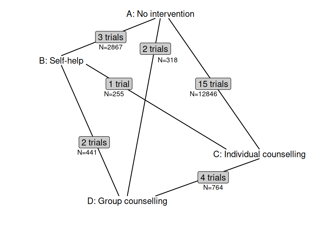
The comparison C vs A is very prevalent and there are 15 trials for it, with an overall sample size of over 12 800 individuals. In contrast, there is only one trial comparison B to C, with only 255 people in total.

In addition, because the measure of “success” for a given intervention is defined as “quit smoking within 6-12 months”, we may expect some heterogeneity in the outcomes – studies associated with a shorter follow-up may over-estimate the probability of success, as it is perhaps harder to maintain smoking cessation in the long-run; or perhaps it is possible that once a certain amount of time has passed without smoking, then perhaps individuals have effectively quit smoking for good and thus the studies with shorter follow-up may actual under-estimate the relevant success rates. We return to this point in Example 7.2.

7.2.1 Fixed effect NMA

We start by considering a “fixed effect” NMA – this is an extension to the “complete pooling” model discussed in Section 6.2.2. In particular, the log odds of the response in each arm is modelled as a function of the effect of study \(s\) plus the incremental effect of treatment \(t\), for \(s = 1, \ldots, S\), different values of \(t\) in each \(s\). \[ \begin{aligned} & r_{st} \sim \text{Binomial}(\pi_{st},n_{st}) \\ & \text{logit}(\pi_{st}) =\alpha_s + \delta_{st} \\ & \delta_{st} = d_t - d_{b_{s}}. \end{aligned} \] Here, \(b_s\) is a variable that describes the treatment arm chosen as reference in each study \(s\) – see Note 7.1 below for more description of the indexing of the relevant variables in the model. We artificially order the interventions so that whenever the “No intervention” (\(t=1\)) option is available, then it is considered as the reference category. If it is not (e.g. in study 23, where \(t=3,4\): Group and Individual counselling are compared), then we assume the one with the lower index (in that case \(t=3=\) Individual counselling) to be the reference – see the discussion in Note 6.1 in Example 6.1.

We complete the model by placing suitable prior distributions on the parameters. The quantities \(\alpha_s\) are defined as the study-specific baseline probability for smoking cessation in the treatment arm that is the reference for that particular study, on the logit scale. We model them as \(\alpha_s\sim\text{Normal}(0,\text{sd}=10)\), which implies a large enough variance – when rescaled to \([0;1]\), this means that, in the prior, 95% of the mass is effectively included in the whole range.

As for the log ORs, we first set \(d_1=0\) and then model \(d_t\sim\text{Normal}(0,\text{sd}=1)\), for \(t=2,\ldots,T\). This construction amounts to fixing the “No intervention” arm as having no incremental effect over the “untreated population” chances of quitting smoking (as seems reasonable), while allowing the other interventions to have an incremental effect. The choice of the relatively informative standard deviation is again perhaps a red herring: in fact, we can use Monte Carlo simulations to check what the prior range is on the natural scale (i.e. for the ORs), using the following code.

rnorm(100000,0,1) |> exp() |> bmhe::stats()

     mean        sd      2.5%    median     97.5% 
1.6373945 2.1246894 0.1414384 0.9949352 7.0545545 

As is possible to see, even with this seemingly tight prior, we are allowing for most of the mass in the OR distributions to be in a very wide range, i.e. ORs as large as over 7!

NoteViva Jacob Bernoulli!

Notice that while it is obviously possible that a different distribution is more suitable to model sampling variability for the observed data, in the case of NMAs, it is often the case that the reported summary statistics available from the SLR come in the form of counts for cases over a number of individuals and thus the Binomial model (originally developed by the Swiss mathematician Jacob Bernoulli, in work published posthumously, in 1713) applies naturally.

Extensions are obviously possible, for instance using a Normal model to describe the data and a linear predictor for their mean (see for instance the model for the data presented in Table 9.1), or a Poisson distribution to model sampling variability and a log linear predictor for the mean or the rates. The basic modelling principles described here, however, also apply virtually unchanged.

Example 7.2. Smoking cessation (continued): fixed effect NMA. In order to map the modelling assumptions into suitable JAGS code, we can efficiently restructure the dataset from the format presented in Table 7.1. In particular, we turn it into a “long-format”, i.e. we wrangle the data so that there are multiple rows for each study, one for each intervention involved in it. Table 7.2 shows the resulting dataset, which we save in an object named smoking_data, in our R workspace.

Table 7.2: An excerpt of the “long-format” dataset. The 24 original studies get expanded into 50 rows, because there are at least two rows for each study (one per comparator). The two three-armed studies contribute three rows each

ID \(i\)	Study \(s\)	Quitters \(r\)	Participants \(n\)	Intervention \(t\)	Baseline \(b\)
1	1	79	702	1	1
2	1	77	694	2	1
3	2	18	671	1	1
4	2	21	535	2	1
\(\ldots\)	\(\ldots\)	\(\ldots\)	\(\ldots\)	\(\ldots\)	\(\ldots\)
47	23	12	76	3	3
48	23	20	74	4	3
49	24	9	55	3	3
50	24	3	26	4	3

The variable \(s\) indicates the study: for instance, study 1 is indexed in the first two rows. The variables \(r\) and \(n\) give the number of quitters and participants associated with the treatment arm described in variable \(t\); thus, in the first row, we collect \(r=79\) and \(n=702\), for treatment arm 1 (No intervention), while in the second one, the numbers are those for treatment arm 2 (Self-help), which is the other intervention considered in study 1. Finally, the variable \(b\) is the baseline treatment arm for that particular study, as described above.

We then code up a complete pooling/fixed effect model, to estimate the relative effects (in terms of log-odds ratios, d[t]).

smoking_fe=function(){
  for (i in 1:N) {
    r[i] ~ dbin(pi[i],n[i])
    logit(pi[i]) <- alpha[s[i]] + delta[s[i],t[i]]
    delta[s[i],t[i]] <- d[t[i]] - d[b[i]]
  }
  
# Prior for baseline log-odds
  for (s in 1:S){
    alpha[s] ~ dnorm(0,0.01)
  }
# Prior for the incremental effects (log-OR)  
  d[1] <- 0  # log odds ratio compared to treatment 1 (e.g. placebo)
  for (t in 2:T) {
    d[t] ~ dnorm(0,1)
  }

# Maps odds ratios for *all* treatment comparisons
  for (A in 1:(T-1)) {
    for (B in (A+1):T)  {
      or[A,B] <- exp(d[A] - d[B])
      or[B,A] <- 1/or[A,B]
    }
  }
# Log odds of quitting successfully under no intervention (from published data)
  rho ~ dnorm(-2.6, 6.925208) # = SD 0.38
# Absolute probability of quitting successfully under each intervention
  for (t in 1:T) {
    logit(p[t]) <- rho + d[t]
  }
}

Note 7.1: Nested indices and long-format datasets

If a dataset is “rectangular”, i.e. it has the form of a matrix, where all the variables have the same number of observations, then it is easy to map the mathematical expressions (e.g. \(d_{st}\)) in matrix format, using multi-dimensional arrays. In the simplest case, these are just two-dimensional matrices.

However, not uncommonly, the available data do not quite follow this simple pattern and it is possible that there are different sizes – for instance, in the dataset shown in Table 7.1, the number of arms is not always equal to 2 and, in addition, the arms considered in a given study are not always the same.

For this reason, it is helpful to work with “nested indices” and long-format datasets, as in Table 7.2 so that for each row (or value of the main index i), we can use the ancillary indexing variables t or b to correctly specify the data. For instance, for i=4, the notation

logit(pi[i]) <- alpha[s[i]] + delta[s[i],t[i]]
delta[s[i],t[i]] <- d[t[i]] - d[b[i]]

translates into

logit(pi[4]) <- alpha[2] + delta[2,2]
delta[2,2] <- d[2] - d[1]

correctly indicating that the incremental effect \(\delta_{2\,2}\) is modelled for intervention \(t=2\) over the baseline considered in study \(s=2\), i.e. the first intervention and therefore the log OR is \(d_2-d_1\).

We also construct the ORs for all the pairwise comparisons of interest – we do this by rescaling the log ORs. We use two loops and compute the ORs in both directions, e.g. \(\text{OR}_{\text{A},\text{B}}\) as well as \(\text{OR}_{\text{B},\text{A}}\).

Finally, we also estimate the absolute probability of quitting smoking under each intervention. To do so, we first use evidence from the published literature to estimate this probability in the “No intervention” scenario. This suggests a probability of around 7% with an upper limit of 14% for the probability of quitting without any other intervention being put in place.

We elicit this in the variable \[\rho\sim\text{Normal}\left(\text{logit}(0.07),\text{sd}=\frac{\text{logit}(0.14)-\text{logit}(0.07)}{2}\approx 0.38\right), \tag{7.1}\] cfr. Section 1.2.5. This allows us to construct an estimate of the absolute probability of quitting \[p_t=\frac{\exp(\rho+d_t)}{1+\exp(\rho+d_t)},\] for each \(t=1,\ldots,T\) – recall that \(d_1=0\) and so \(p_1=\exp(\rho)/\left[1+\exp(\rho)\right]\).

NoteModelling baseline outcomes

The choice for the baseline logit-scale probability of quitting smoking (i.e. when no intervention is active and people are left to their own devices) selected in Equation 7.1 is obviously not unique. For instance, Baio et al. (2025) use some sort of average of the “No intervention” arm treatment effect, computed as \[ \rho = \frac{1}{\sum_{s=1}^S\mathbb{I}(b_s=1)}\sum_{s\in\mathbb{I}(b_s=1)}\alpha_s, \] where \(\mathbb{I}(b_s=1)\) is the set of studies in which the “No intervention” arm is observed (i.e. studies 1 to 19, in Table 7.1).

Another alternative, perhaps more model-based, would be to distinguish the effect for the “No intervention” arm by modelling the relevant parameter using some partial pooling model, so as to automatically derive a pooled estimate for the baseline probability of quitting smoking.

Equation 7.1 has the advantage of producing an estimate that is, potentially, based on consistent evidence from external data, thus providing a prior distribution that may be more robust against potential selection bias issues present in the \(S\) studies.

We finally define the data list with the relevant variables and then run the model using JAGS. We select a relatively long burn-in phase of 5000 iterations and also run the MCMC for 25 000 iterations, with thinning of 10, which means we use 4000 simulations for our MC analysis.

# Data list
data.list=list(
  t=smoking_data$t,             # Treatment indicator
  s=smoking_data$s,             # Study indicator
  r=smoking_data$r,             # Observed number of quitters
  n=smoking_data$n,             # Total sample size in study s
  b=smoking_data$b,             # Baseline intervention in study s
  N=smoking_data |> nrow(),     # Number of rows in the data
  T=smoking_data$t |> max(),    # Total number of treatment arms
  S=smoking_data$s |> max()     # Total number of studies
)
# Runs model
m_fe=jags(
  data=data.list,parameters.to.save=c("d","or","p"),n.thin=10,
  inits=NULL,n.chains=2,n.burnin=5000,n.iter=25000,model.file=smoking_fe
)

We can check convergence and autocorrelation, as usual (for example, as detailed in Section 3.2). In this case, all is in order, with all the relevant nodes having a value of the PSR statistic well below 1.1 and with reasonably large effective sample size, although some parameters do present a non-zero level of autocorrelation.

In this particular case, we have the advantage that we can check the consistency of all the indirect comparisons we obtain by pooling together all the data, with the estimates we could obtain from a version of the model in which each pairwise comparison is only informed by the studies in which it is observed (and not indirectly from all the others).

We can do this by modifying the JAGS code used for the general fixed effects model to the following

d[1] <- 0  # log odds ratio compared to treatment 1 (e.g. placebo)
for (t in 2:T) {
  d[t] ~ dnorm(0,1)
}
or <- exp(d[Active] - d[Baseline])

– note that we pass Active and Baseline as numerical indices for the “active” or “baseline” intervention respectively, in the modified data list; for example, to compare C vs B, we would select Active=3 and Baseline=2. For each combination of Active and Baseline, we restrict the dataset to only those studies that compare these two options directly.

Figure 7.2: Summary of the posterior distributions for the pairwise comparisons, using the no pooling model (to only consider direct evidence) and the complete pooling (“fixed effect”), which uses all the evidence, including indirect.

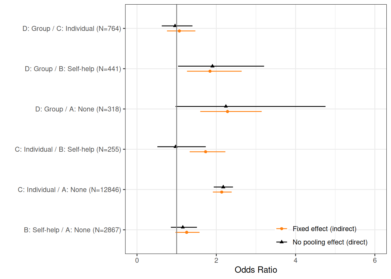
Figure 7.2 compares the no-pooling model (“direct evidence”) with the fixed effect one (“indirect evidence”). As is possible to see, some of the pairwise comparisons are very much aligned; for instance, the estimates for the comparison between C and A are basically identical. This is not surprising, as there are a large number of aggregated observations (over 12 800), to directly obtain them.

In the case of comparisons directly informed by fewer data, the differences between direct and indirect estimates are more striking: the precision for the comparison between D and A is improved by the indirect data for C vs A and C vs D, which pool together a large sample size.

As for the case of C vs B, the direct effect is substantially different than the indirect one. This is because the direct evidence is only from two relatively small studies (\(s=20,21\)) and therefore the indirect estimate is pulled towards the much bigger indirect C vs A and B vs A data. This suggests some evidence of heterogeneity.

We can also get a better sense of the underlying differences in the individual studies, by running a “no-pooling” model (see Section 6.2.1). In this case, we modify the code for the fixed effect model as in the following JAGS code.

# Model code for no-pooling individual studies
heterogeneity=function() {
  for (i in 1:N) {
    r[i] ~ dbin(pi[i],n[i])
    logit(pi[i]) <- alpha[s[i]] + delta[s[i],t[i]]
    delta[s[i],t[i]] <- d[s[i],t[i]] - d[s[i],b[i]]
  }
  for (s in 1:S) {
    alpha[s] ~ dnorm(0,0.01)
    d[s,1] <- 0
    for (j in 2:4) {
      d[s,j] ~ dnorm(0,1)
    }
    or[s] <- exp(d[s,Active] - d[s,Baseline])
  }
}

In this model, we now consider study- and treatment-specific differential effects \(d_{st}\), to be able to estimate an OR for each combination. Notice that some of the studies are informed by very little data (e.g. \(s=19\)), which contributes to large variance, especially in the face of rather vague priors – we could probably do a better job by regularising the prior range for the ORs, e.g. by increasing the precision for \(d_{st}\). As we are not really using this model for inference, but rather just to gauge the underlying heterogeneity, we just consider the “basic” model, which is consistent with the rest of our analysis.

Figure 7.3: Summaries for the posterior distribution of the ORs for all the relevant pairwise comparisons, using direct evidence only and for a no-pooling model. The \(x\)–axis is on a log scale; on the \(y\)–axis, the study index \(s\) and overall sample size \(N\) are also reported.

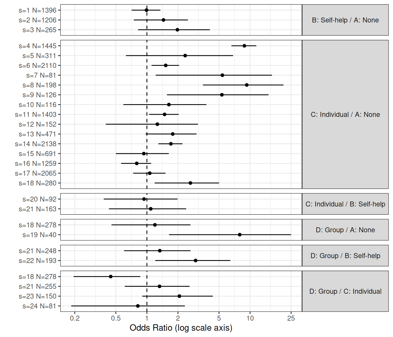
Figure 7.3 shows the result of this no-pooling model. As is possible to see, there is very large heterogeneity even within studies characterised by the same comparison. In particular, there are quite a few estimates that return a very large OR and uncertainty around the central estimate that is larger still (notice that the \(x\)–axis is expressed on a log scale). As is obvious, heterogeneity as well as the precision for the estimates (measured by how tight the intervals around the mean estimates are) depends inversely on the total sample size; so, for instance, smaller studies will be associated with larger variance.

This strongly suggests that we should consider very seriously a partial-pooling version (see Section 6.2.3) of the NMA, to better account for the underlying heterogeneity in the data.

7.2.2 Random effects NMA

To expand to a random effect structure, in line with Section 6.2.3, we need to model the log ORs as exchangeable, which we can do by assuming \[ \begin{aligned} \delta_{st} & \sim \text{Normal}(\mu_{st},\sigma_{st}) \\ \mu_{st} & = d_t-d_{b_{s}} \\ \sigma_{st} & \sim p(\sigma_{st}). \end{aligned} \tag{7.2}\]

In contrast to the simplest case of meta-analysis/evidence synthesis discussed in Chapter 6, in a NMA there are \(T\) different treatments and \((T - 1)\) different pooled effects, relative to treatment 1 (the baseline / reference). We can, in principle, assume that there are \((T-1)\) different random effects distributions to estimate – but often this will not be feasible, unless a large enough number of studies for every single treatment is available.

This means that we generally need to add some identifiability constraints, e.g. by making assumptions such as that the random effects standard deviation is the same for each treatment comparison: \(\sigma_{st} = \sigma\). Of course, if we had strong prior knowledge or expectation of differing amounts of heterogeneity for different treatment effects, we should not make this assumption and suitable extensions to this model have been proposed in the literature (Lu and Ades, 2004, 2006) – see also Dias et al. (2018, pp. 35–50) for more details and code suggestions.

Example 7.3. Smoking cessation (continued): random effect NMA. To complete the random effect NMA specified in Equation 7.2, we need to define a prior distribution for the random effect standard deviation on the log ORs. We could use one of the models shown previously, e.g. an Exponential PC prior (with the parameter \(\lambda\) defined to elicit a suitable tail-area probability for \(\sigma\)).

In this case, we consider the Half-Cauchy prior suggested by Gelman (2006). In particular, while the Cauchy distribution is not directly implemented in JAGS, we can use its mathematical properties to prove that \[ y\sim \text{Half Cauchy}(\mu=0,\lambda) = \text{t}(\mu=0,\tau,\nu=1)\mathbb{I}(0,\infty) \] where \(\lambda\) is a scale parameter and \(\tau=\lambda^{-2}\) is the precision (cfr. Equations 1.5 and 6.9). Consequently, “truncating” a \(\text{t}\) distribution with mean \(\mu=0\), precision \(\tau\) and \(\nu=1\) degree of freedom to only take on \(\mathbb{R}^+\) provides the required prior.

NoteTruncated distributions

In a nutshell, a variable \(y\) defined in a full range \(\mathcal{Y}\) (e.g. \(\mathbb{R}\)) is “truncated” in a given interval \(\mathcal{I}\subset \mathcal{Y}\) (e.g. \(\mathbb{R}^+\)) if \[ y\sim\left\{\begin{array}{cc} p(y\mid\boldsymbol\theta) & \text{if $y\in \mathcal{I}$} \\ 0 & \text{if $y \notin \mathcal{I}$}, \end{array}\right. \] i.e., for some reason, \(y\) is only observed in a subset of its full theoretical range.

Because of this quirk, the distribution \(p(y\mid\boldsymbol\theta)\) needs to be re-normalised dividing by \(\Pr(Y\in\mathcal{I})\), in order to retrieve the correct contribution to the likelihood – in other words, if \((a,b)\) are the lower and upper bounds of the interval \(\mathcal{I}\), then \[ y\sim \frac{p(y\mid\boldsymbol\theta)}{\Pr(Y\in\mathcal{I})}=\frac{p(y\mid\boldsymbol\theta)}{F(b\mid\boldsymbol\theta)-F(a\mid\boldsymbol\theta)}. \]

In JAGS, this is achieved through the T(,) operator – for instance, the code

sigma ~ dt(0,0.04,1)T(0,)

implies a \(\text{Half Cauchy}(0,5)\) model for a variable sigma – in line with the parameterisation used in Equation 1.5, in JAGS the t distribution is indexed by the precision. Thus a value of 0.04 for the precision \(\tau\) of the t distribution implies a scale \(\lambda=\tau^{-0.5}=5\) for the resulting Half Cauchy.

In particular, we specify \(\sigma \sim \text{Half Cauchy}(0,2)=\text{t}(0,0.25,1)\mathbb{I}(0,\infty)\). This prior can be visualised in Figure 7.4, where we have also overlaid an \(\text{Exponential}(0.4)\) – this would amount to a PC prior for which \(\Pr(\sigma>6)\approx 0.1\).

Figure 7.4: Comparison of a Half Cauchy(0,2) and an Exponential(0.4) prior distributions for \(\sigma\).

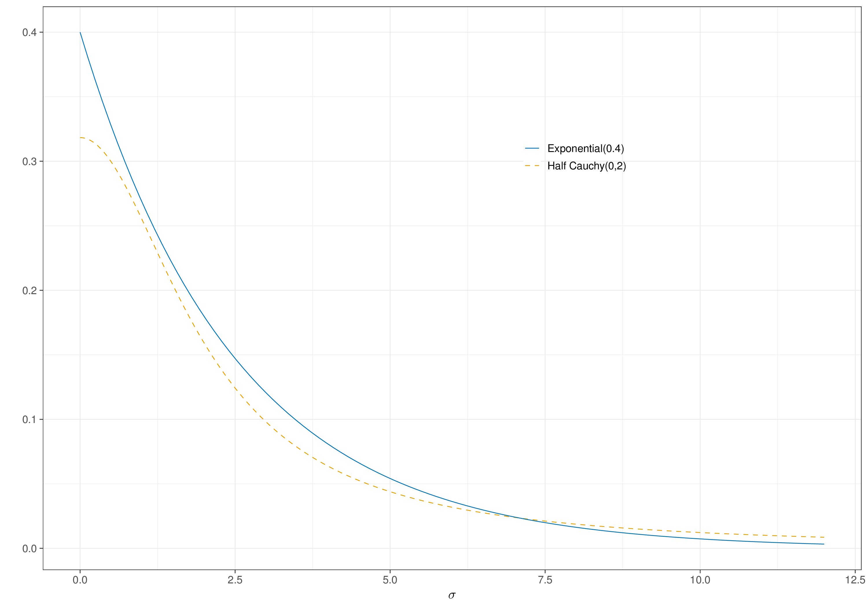
The two priors are reasonably aligned – this means that by assuming the Half Cauchy(0,2), we are also implying a very small chance that the random effects standard deviation would exceed a rather large value such as 6; we can use forward sampling (see Section 1.2.6) to estimate that in fact \(\Pr(\sigma>6)\approx 0.102\) for the Half Cauchy prior.

Note Mean-precision \(\text{t}\) distribution in R

In R, the built-in commands to compute the density and cumulative distribution for, or to sample from a \(\text{t}\) distribution (respectively, dt, pt and rt) are based on a different parameterisation, in comparison to the one we use here (see Equation 1.5). More specifically, R implicitly fixes \(\mu\equiv 0\) and \(\tau\equiv 1\), while BUGS/JAGS allow different values for the parameters – basically, if \(y\sim\text{t}(\mu,\tau,\nu)\) and \(z\sim\text{t}(\mu\equiv 0,\tau\equiv 1,\nu)\) then \(z=(y-\mu)\sqrt{\tau}\).

Consequently, the mean-precision version of the \(\text{t}\) density and cumulative density can be obtained from the R parameterisations, which we indicate respectively as \(p^*(\cdot\mid\nu)\) and \(F^*(\cdot\mid\nu)\), applying the rule for change of variable. This yields the following transformations \[ p(y\mid\mu,\tau,\nu)=\sqrt{\tau} p^*\!\!\left(\sqrt{\tau}(y-\mu)\mid\nu\right) \quad \text{and} \quad F(y\mid\mu,\tau,\nu)=F^*\!\!\left(\sqrt{\tau}(y-\mu)\mid\nu\right), \] which, in R are obtained using the following commands.

density=sqrt(tau)*dt(sqrt(tau)*(y-mu),nu)
cum_dist=pt(sqrt(tau)*(y-mu),nu)

We can code up the full random effect NMA model specified above using the following.

smoking_re=function(){
  for (i in 1:N) {
    r[i] ~ dbin(pi[i],n[i])
    logit(pi[i]) <- alpha[s[i]] + delta[s[i],t[i]]
    delta[s[i],t[i]] ~ dnorm(mu[s[i],t[i]],tau)
    mu[s[i],t[i]] <- d[t[i]] - d[b[i]]
  }
  
# Prior for baseline log-odds
  for (s in 1:S){
    alpha[s] ~ dnorm(0,0.01)
  }
# Prior for the incremental effects (log-OR)  
  d[1] <- 0  # log odds ratio compared to treatment 1 (e.g. placebo)
  for (t in 2:T) {
    d[t] ~ dnorm(0,1)
  }
# Half-Cauchy prior for common sd for the random effects. NB: in JAGS, the 
# t distribution is indexed in terms of the *precision* (=1/variance)!
  sigma ~ dt(0,0.25,1)%_%T(0,)
  tau <- pow(sigma,-2)

# Maps odds ratios for all treatment comparisons
  for (A in 1:(T-1)) {
    for (B in (A+1):T)  {
      or[A,B] <- exp(d[A] - d[B])
      or[B,A] <- 1/or[A,B]
    }
  }
# Log odds of quitting successfully under no intervention (from published data)
  rho ~ dnorm(-2.6,6.925208) # = SD 0.38
# Absolute probability of quitting successfully under each intervention
  for (t in 1:T) {
    logit(p[t]) <- rho + d[t]
  }
}

Note 7.2: Using truncation in JAGS model code (passed as a function)

Throughout the examples in the book, we have constructed the JAGS model code as an R function. In the case of the model above, we must include the “truncation” operator T(0,), which instructs JAGS to only simulate values for the underlying \(\text{t}(\mu,\tau,\nu)\) distribution from \(\mathbb{R}^+\) and applies the suitable rescaling of the density.

However, the use of the string

sigma.delta ~ dt(...)T(0,)

within a function is incompatible with R syntax and thus it would break the code, throwing an R error such as the following.

Error: unexpected symbol in:
"# Half-Cauchy prior for common sd for the random effects
  sigma.delta ~ dt(0,0.25,1)T"

To avoid this issue, when defining the function containing the model code, e.g. smoking_re() above, we use a dummy operator %_% before the truncation code. This gets automatically parsed out when running R2jags::jags(), through the function R2WinBUGS::write.model(), which is called in the background to write the model code to a temporary file.

The model can be run using the following R code. We again use a burn-in phase of 5000 iterations and run the MCMC for 25 000 iterations, with thinning of 10.

# Runs model
m_re=jags(
  data=data.list,parameters.to.save=c("d","or","p","sigma"),n.thin=10,
  inits=NULL,n.chains=2,n.burnin=5000,n.iter=25000,model.file=smoking_re
)

Figure 7.5 depicts diagnostics for the model, in terms of the PSR and effective sample size. Generally speaking, we can be satisfied with convergence and the level of autocorrelation does not appear too much of a concern.

(a) \(\hat{R}.\)

(b) \(n_{\text{\textit{eff}}}\).

Figure 7.5: Diagnostic plots for the random effects NMA.

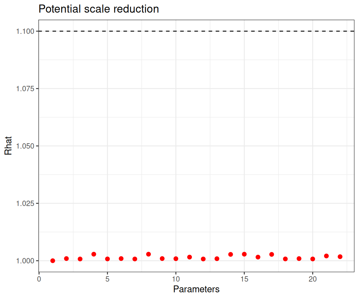
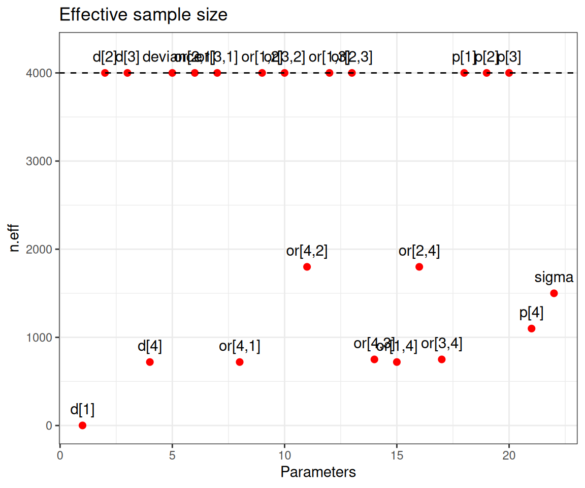
Convergence is not an issue in this model and all the main parameters are associated with sufficiently large effective sample size.

We can compare the fixed and random effects NMA, using for instance the DIC. In this case, the complete pooling model is associated with a DIC of 520.8, while the corresponding value for the partial pooling model is 335.8. This large difference, confirms the presence of large heterogeneity in the underlying studies and thus justifies the use of the random effect NMA. More specifically, the amount of shrinkage in the partial pooling model can be computed as a reduction of 43.62% in the number of model parameters (from a nominal 79 to the effective 44.54 parameters, as measured by \(p_D\)) – see the discussion in Section 6.2.7.

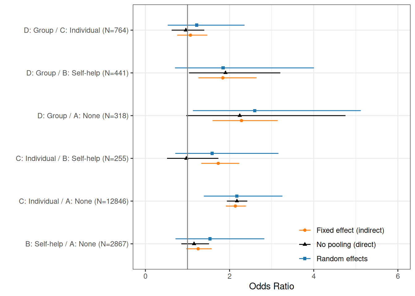
Figure 7.6 shows a full comparison of the direct and indirect evidence, using both a fixed and a random effects NMA. Generally speaking, the random effects model is associated with wider intervals, after accounting for heterogeneity. While this may sound as a “disappointing” result, perhaps a more appropriate phrasing would be that, in fact, it is the fixed effects model that tends to give artificially tight interval estimates, which do not fully reflect the underlying variability in the studies.

The comparison between C and B shows that the random effect model is a “compromise” between the direct and indirect evidence, while for D vs A, as it is based on the smallest trials, there is still substantial uncertainty.

Figure 7.6: Comparison of the three versions of the NMA. The partial pooling (“random effects”) generally acts as a compromise between the two extremes of the no- and complete-pooling models. Generally speaking, the uncertainty is higher in the partial pooling model, because of the underlying large heterogeneity inherent in the \(S\) studies, which is artificially discarded in the two other models.

7.3 Economic evaluation based on NMA

Generally speaking, the NMA process will be specifically designed to obtain pooled estimates for some relevant relative effects and we will want to propagate the inherent uncertainty through some suitable economic model, to obtain estimates for suitable population average benefits and costs and then perform the usual economic analysis.

The power of the Bayesian machinery is that, once the statistical model is fitted, then the remaining steps are more or less repeated in a similar fashion – the propagation of the uncertainty and the PSA come almost for free (see the discussion in Chapter 4).

Example 7.4. Smoking cessation (continued): economic evaluation. We first turn the estimates for the relative effects obtained in the NMA into suitable absolute effects (see the discussion in Note 6.1 in Chapter 6).

Considering the fixed and random effect models to pool all the available evidence (both direct and indirect), we can automatically consider the nodes p[t] defined both in the smoking_fe() and smoking_re() model code functions. These represent estimates of the absolute probability of quitting smoking, under each of the \(T=4\) interventions considered.

Figure 7.7 compares the posterior distributions under the two models. The numbers indicate the estimates for the 95% interval and the posterior mean – note that the estimates for the “No intervention” arm are essentially identical (up to Monte Carlo simulation error). This is correct, because in both the fixed and random effect models, this baseline probability is modelled using the informative prior on the parameter \(\rho\).

Figure 7.7: Estimates for the absolute probability of quitting smoking for the \(T=4\) competing interventions and under the “fixed” and “random” effect models.

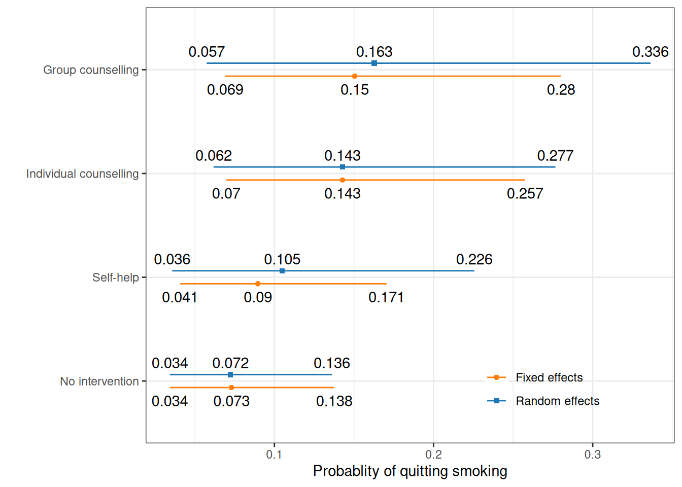
In Figure 7.7, the random effect model produces generally larger intervals, which again reflects the higher uncertainty due to the proper accounting of the underlying heterogeneity in the \(S\) studies.

We can use these results and complement them with external data to obtain a measure of clinical benefit from quitting smoking, in terms of life years gained. Specifically, this will vary depending on the age of individuals, with larger benefits encountered for quitters of younger age.

Just to fix ideas, we can consider the results by Mamun et al. (2004), who using the long-running Framingham Heart Study cohort, report increased survival in years of 8.66 (95% interval \([7.61; 9.63]\)) and 7.59 (95% interval \([6.33; 8.92]\)), for men and women, respectively. In addition, using official statistics (e.g. from the UK Office for National Statistics), we can derive the gender distribution of smokers – for instance, ONS (2024) suggest that, in 2023, smokers in the UK were distributed as 3.4 million men and 2.6 million women, which implies a proportional split of 56.67:43.33.

If we model the uncertainty in the life years gained using suitable Normal distributions centred on the point estimates and with standard deviations computed as in Section 1.2.5, we can derive an estimate for the extra life years gained by not smoking (i.e. for quitters) as \(l_m\sim\text{Normal}(\text{mean}=8.66, \text{sd}=0.495)\) for men and \(l_f\sim\text{Normal}(\text{mean}=7.59, \text{sd}=0.679)\) for women, respectively. It is easy to check through Monte Carlo simulations that these distributions match closely the interval estimates provided by Mamun et al. (2004).

We can combine these two distributions with weights \(w_m=0.567\) and \(w_f=0.433\) into our final estimate for the overall life years gained as \(l= w_m l_m + w_f l_f\) and then derive an intervention-specific measure of clinical benefit as \(e_t = p_t l\). We can use the output from our models (and in fact, we consider here only the random effect one) and Monte Carlo simulations, as demonstrated in the following R code.

# First computes the life years gained
lm=rnorm(m_re$BUGSoutput$n.sims,8.66,0.495)
lf=rnorm(m_re$BUGSoutput$n.sims,7.59,0.679)
l=0.567*lm + 0.433*lf

# Then weighs these with the probability of quitting for each intervention
e=m_re$BUGSoutput$sims.list$p * l
labs=c(
  "No intervention","Self-help","Individual counselling","Group counselling"
)
# And shows some summary statistics of the resulting distribution
e |> bmhe::stats() |> (\(x) {rownames(x)=labs; x})()

                            mean        sd      2.5%    median    97.5%
No intervention        0.5933977 0.2201685 0.2778440 0.5594116 1.132097
Self-help              0.8599951 0.4082487 0.2910501 0.7807603 1.855900
Individual counselling 1.1705738 0.4510420 0.5084005 1.1000942 2.253484
Group counselling      1.3337088 0.5995808 0.4718871 1.2351707 2.776559

Note 7.3: Piping functions

Notice that, in R, the code (\(x) ...)() can be used as a shortcut for defining a function func(x){...}. Here we first consider the object e, then we apply the function bmhe::stats() to it, to compute the summary statistics from the posterior distributions and then we “pipe” a function to define the names of the four rows of the resulting matrix.

As for the costs, we consider the analysis in Baio et al. (2025), based on the data provided in Table 7.3, which can be used to determine a central estimate for the overall cost of implementation of each of the interventions. Note that, in a more comprehensive evaluation, we would perhaps need to consider more resources that directly impact on the individuals’ quality of life, such as complications (e.g. acute and chronic treatment of cardiovascular disease and events). Here, we keep the modelling relatively simple and only use the direct cost of implementation of the four interventions.

Table 7.3: Point estimates (in £) for the costs associated with the \(T=4\) interventions considered in the smoking cessation example

Intervention	Item cost (in £)	Total cost (£)
No intervention	---	0.0
Self-help	Nicotine replacement therapy (NRT) for five weeks (35 patches at 1.30 each)	45.5
Individual counselling	NRT for five weeks (35 patches at 1.30 each) + five clinic visits (10 each)	95.5
Group counselling	NRT for five weeks (35 patches at 1.30 each) + five clinic visits (19.46 each)	142.8

In addition, to account for variance in compliance and potential side treatments, we associate each of the costs with a probability distribution, for the three “active” interventions. In particular, we consider Gamma distributions where the mean is set to the observed total cost and the standard deviation is fixed at 30% of that amount. This is a relatively common practice in HTA, where, in the absence of genuine information, the central estimate is perturbed assuming some fixed value for the underlying coefficient of variation \(\text{CV}=\mu/\sigma\) – this effectively implies that the standard deviation \(\sigma\) is set to a fraction of the estimated mean \(\mu\).

We can use the function bmhe::gammaPar() to return the shape and rate parameters for a Gamma distribution to match given values for the underlying mean and standard deviation – other examples for this kind of strategy are presented in Example 9.3. For example, the code

bmhe::gammaPar(45.5,.3*45.5)

$shape
[1] 11.11111

$rate
[1] 0.2442002

bmhe::gammaPar(45.5,.3*45.5) |> 
  (\(x) rgamma(100000,shape=x$shape,rate=x$rate))() |> bmhe::stats()

    mean       sd     2.5%   median    97.5% 
45.55988 13.66090 22.86102 44.20328 75.86362 

suggests that modelling \(c_2\sim\text{Gamma}(\text{shape}=11.111,\text{rate}=0.244)\) would have, at least approximately the required properties. Similar reasoning allows us to model the costs for the individual and group counselling using \(c_3\sim\text{Gamma}(\text{shape}=11.111,\text{rate}=0.116)\) and \(c_4\sim\text{Gamma}(\text{shape}=11.111,\text{rate}=0.078)\), respectively.

As for the “No intervention” arm, if we do not consider relevant outcomes (such as hospitalisations for major cardiovascular events), we keep the cost of implementation to £0, with no variance. In reality, as mentioned above, we would include costs borne by the healthcare provider for resource use related to the underlying condition, e.g. to treat acute heart conditions, which would also impact on the benefit side.

We can then bring all these elements together and perform the cost-effectiveness analysis, for instance using the following R code – notice that we could include these calculations inside the JAGS object, but since these are pure forward sampling, it would have no effect on the actual estimates based on the computing the posterior distributions for the actual model parameters.

# Defines the matrix of cost simulations
c=matrix(
  c(
    rep(0,m_re$BUGSoutput$n.sims),
    rgamma(m_re$BUGSoutput$n.sims,shape=11.111,rate=0.244),
    rgamma(m_re$BUGSoutput$n.sims,shape=11.111,rate=0.116),
    rgamma(m_re$BUGSoutput$n.sims,shape=11.111,rate=0.078)
  ),
  nrow=m_re$BUGSoutput$n.sims,ncol=4
)

# Runs BCEA to perform the economic evaluation
library(BCEA)
m=bcea(e,c,ref=4,Kmax=4000,interventions=labs)
summary(m)

NB: k (wtp) is defined in the interval [0 - 4000]

Cost-effectiveness analysis summary 

Reference intervention:  Group counselling
Comparator intervention(s): No intervention
                          : Self-help
                          : Individual counselling

Optimal decision: choose No intervention for k < 168
                         Individual counselling for 168 <= k < 288
                         Group counselling for k >= 288


Analysis for willingness to pay parameter k = 4000

                       Expected net benefit
No intervention                      2373.6
Self-help                            3394.4
Individual counselling               4586.4
Group counselling                    5192.1

                                                EIB    CEAC   ICER
Group counselling vs No intervention        2818.48 0.98200 192.85
Group counselling vs Self-help              1797.70 0.86850 205.09
Group counselling vs Individual counselling  605.69 0.62675 287.21

Optimal intervention (max expected net benefit) for k = 4000: Group counselling
           
EVPI 403.54

As is clear from the summary, depending on the willingness to pay threshold selected, the optimal intervention does change: when \(k\) is less than £168, then do-nothing is the most cost-effective option; Individual counselling becomes the optimal strategy for \(k\in \text{£}[168; 288]\); and then Group counselling is the most cost-effective intervention for \(k>\text{£}288\).

We can also use the tools described in Section 4.3.3 and produce a more thorough analysis for each intervention. We can do this using BCEA specific functions, as demonstrated in the code below.

# Multi-intervention cost-effectiveness analysis
mce=multi.ce(m)

The function multi.ce() computes and plots the probability that each of the interventions being analysed is the most cost-effective and can be then used to produce the cost-effectiveness acceptability frontier (see Section 4.3.3). The resulting object mce can be further processed, e.g. to apply the ceac.plot method to draw the CEAC for each intervention – and the ggplot2 facilities can be used to further customise the resulting graph as shown in Figure 7.8 (a). This shows the probability that each of the options is the most cost-effective, upon varying the willingness to pay threshold.

(a) Pr(\(t\) is the most cost-effective).

(b) Cost-effectiveness efficiency frontier.

Figure 7.8: Multiple intervention cost-effectiveness analysis for the smoking example.

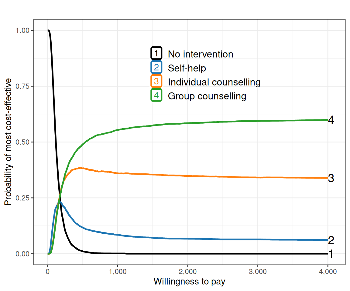
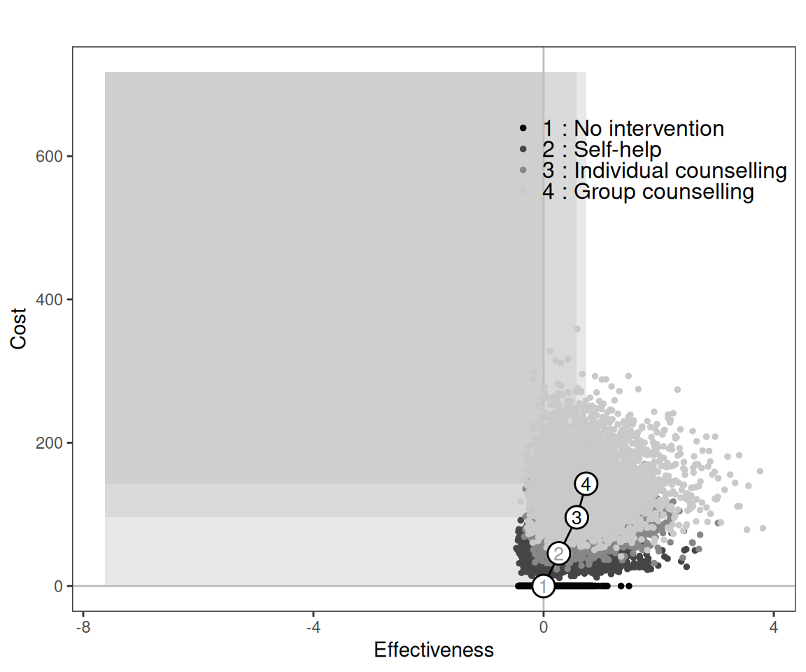
Figure 7.8 (b) shows the cost-effectiveness efficiency frontier and, in line with the discussion above, it shows that “Self-help” is inside the frontier, indicating that, for different threshold values, the other three interventions are optimal.

7.4 Conclusions

In this chapter we have introduced the concept of indirect comparison (which will be reprised in Chapter 11) and expanded on the models developed in Chapter 6 to pool together (summary) data obtained from a number of sources. We have showcased the subtle complexity of NMA through the smoking cessation example, which allowed us to explore the potential implications of the underlying heterogeneity in the data. This has also been expanded into a full economic evaluation, by combining the effectiveness measures obtained through the indirect comparison and suitable information on the cost component.

In the next chapter we concentrate on another extremely popular modelling problem in HTA analyses: the use of time-to-event data (which are the most important outcome for e.g. cancer studies) and survival analysis.

Baio, G., Heath, A., Berardi, A., Green, N., 2025. Bayesian Cost-Effectiveness Analysis with the R Package BCEA, 2nd ed. Springer.

Dias, S., Ades, A., Welton, N., Jansen, J., Sutton, A., 2018. Network Meta-analysis for Decision-making. John Wiley and Sons, Chichester, UK.

Gelman, A., 2006. Prior distributions for variance parameters in hierarchical models. Bayesian Analysis 515–533.

Grant, R., Di Tanna, G.L., 2025. Bayesian meta-analysis: A practical introduction. CRC Press, Boca Raton, FL.

Hasselblad, V., 1998. Meta-analysis of multitreatment studies. Medical Decision Making 18, 37–43.

Jackson, C., 2015. Slides for the Summer School ‘Bayesian methods in health economics’’. URL https://gianluca.statistica.it/teaching/summer-school/

Lu, G., Ades, A., 2006. Assessing evidence inconsistency in mixed treatment comparisons. Journal of the American Statistical Association 101, 447–459.

Lu, G., Ades, A., 2004. Combination of direct and indirect evidence in mixed treatment comparisons. Statistics in Medicine 23, 3105–3124.

Mamun, A.A., Peeters, A., Barendregt, J., Willekens, F., Nusselder, W., Bonneux, L., 2004. Smoking decreases the duration of life lived with and without cardiovascular disease: a life course analysis of the Framingham Heart Study. European Heart Journal 25, 409–415.

Office for National Statistics [ONS], 2024. Adult Smoking Habits in the UK: 2023. URL https://www.ons.gov.uk/releases/adultsmokinghabitsintheuk2023

Welton, N., Sutton, A., Cooper, N., Abrams, K., Ades, A., 2012. Evidence Synthesis for Decision Making in Healthcare. John Wiley and Sons, Chichester, UK.