# Constructs a tibble with the density for the Beta and Uniform priors
# and a range of values from 0 to 1 for the x-axis
priors=tibble(
  theta=seq(from=0, to=1, by=.001),
  p1=dbeta(seq(0,1,.001),9.2,13.8),
  p2=dunif(seq(0,1,.001),0,1)
)
# Plots the densities
priors |> ggplot(aes(theta,p1)) + geom_line()
priors |> ggplot(aes(theta,p2)) + geom_line() 2 Learning from data: Bayesian computation
2.1 Introduction
In Chapter 1 we have considered the main features of Bayesian reasoning and have used Monte Carlo simulations to elicit and manipulate the prior distribution, as well as to propagate the uncertainty in the model parameters onto possible future data, which we have not observed yet, but may be able to do so.
For all intents and purposes, the process of “forward sampling” (see Section 1.2.6) is already fundamentally Bayesian, because it starts with the premise that we are able to map our current epistemic uncertainty on unobservable features of our model through a probability distribution. It is not, however, the full realisation of the Bayesian paradigm, because so far we have not actually used observed data to update our current state of uncertainty on the model parameters – effectively running the process of Bayesian inference from observed data.
To this aim, in this chapter we explore the fundamentals of Bayesian computations as applied to the process of learning from data. We start by considering various choices for the prior distribution; following somewhat the historical patterns that have characterised Bayesian modelling, we start by looking at so-called “vague” priors and the related inferential process. We then consider “conjugate” models, as a slightly less restrictive mode of inference, to then move onto Markov Chain Monte Carlo methods – these have effectively freed up Bayesian computation and rendered it widely applicable, thus constituting a real revolution in statistical modelling.
2.2 Choice of prior distributions
The best way to set a prior distribution is to elicit existing, contextual information (see Section 1.2.2) and to carefully assess the properties of the DGP – for instance, considering whether there is a set of physical properties we need to render with the prior (bounded vs unbounded range, continuous vs discrete, etc.).
In some circumstances, however, we can try and use some “default” priors – these have been historically designed to somehow automate the process of Bayesian inference. They have many merits and should be understood carefully – although, in general, we may be able to do better…
2.2.1 “Vague” priors
To remove some of the sensitivity to the choice of prior (especially in cases where the data do not provide definitive evidence), it is possible to select a distribution that exerts the least amount of impact on the final inference. This type of prior is often referred to as “non-informative” or “vague” and the basic idea is to use a distribution that has a large variance, so as to span more or less uniformly across the entire range of the underlying variable.
A classical example of the use of “vague” priors comes from the work of Pierre Simone Laplace, the French scholar and polymath who is credited to have independently discovered Bayesian modelling (Laplace, 1774, 1812) – see Note 1.2 in Section 1.2. In one of his many applied contributions, Laplace’s research question was about the probability that a new born would be a boy and to investigate this he used data including \(y=241945\) females out of \(n=493527\) babies born and Christened in Paris between 1745 and 1770, with the following modelling assumptions: \[ \begin{aligned} y & \sim \text{Binomial}(\theta,n)\\ \theta & \sim \text{Uniform}(0,1) \end{aligned} \] – note that in general for a variable \(y\) and constants \((a,b)\) \[y\sim\text{Uniform}(a,b) \qquad\Rightarrow\qquad p(y\mid a,b)=\frac{1}{b-a}. \tag{2.1}\]
The choice of a Uniform prior over the entire range of the model parameter \(\theta\) was justified by Laplace on the grounds that he had no real information and so every possible value for \(\theta\) should be equally likely (the principle of insufficient reason)1.
More importantly, choosing a Uniform prior simplifies the computation of the posterior, because \(p(\theta)= c\) (for some positive constant) and thus \[ p(\theta\mid y) = \frac{p(\theta)p(y\mid \theta)}{p(y)} \propto \frac{c\mathcal{L}(\theta\mid y)}{c\int\mathcal{L}(\theta\mid y)d\theta} \propto \frac{\mathcal{L}(\theta\mid y)}{\int \mathcal{L}(\theta\mid y)d\theta}, \tag{2.2}\] i.e. the posterior is proportional to the (rescaled) likelihood function, with essentially no impact of the prior distribution. By using a Uniform prior, Laplace was able to compute analytically the posterior distribution, “simply” by solving an integral calculation. For this reason, vague or Uniform priors have been, historically, the first form of Bayesian modelling (because they would allow the full computation of the posterior distribution in a reasonably wide range of applied cases).
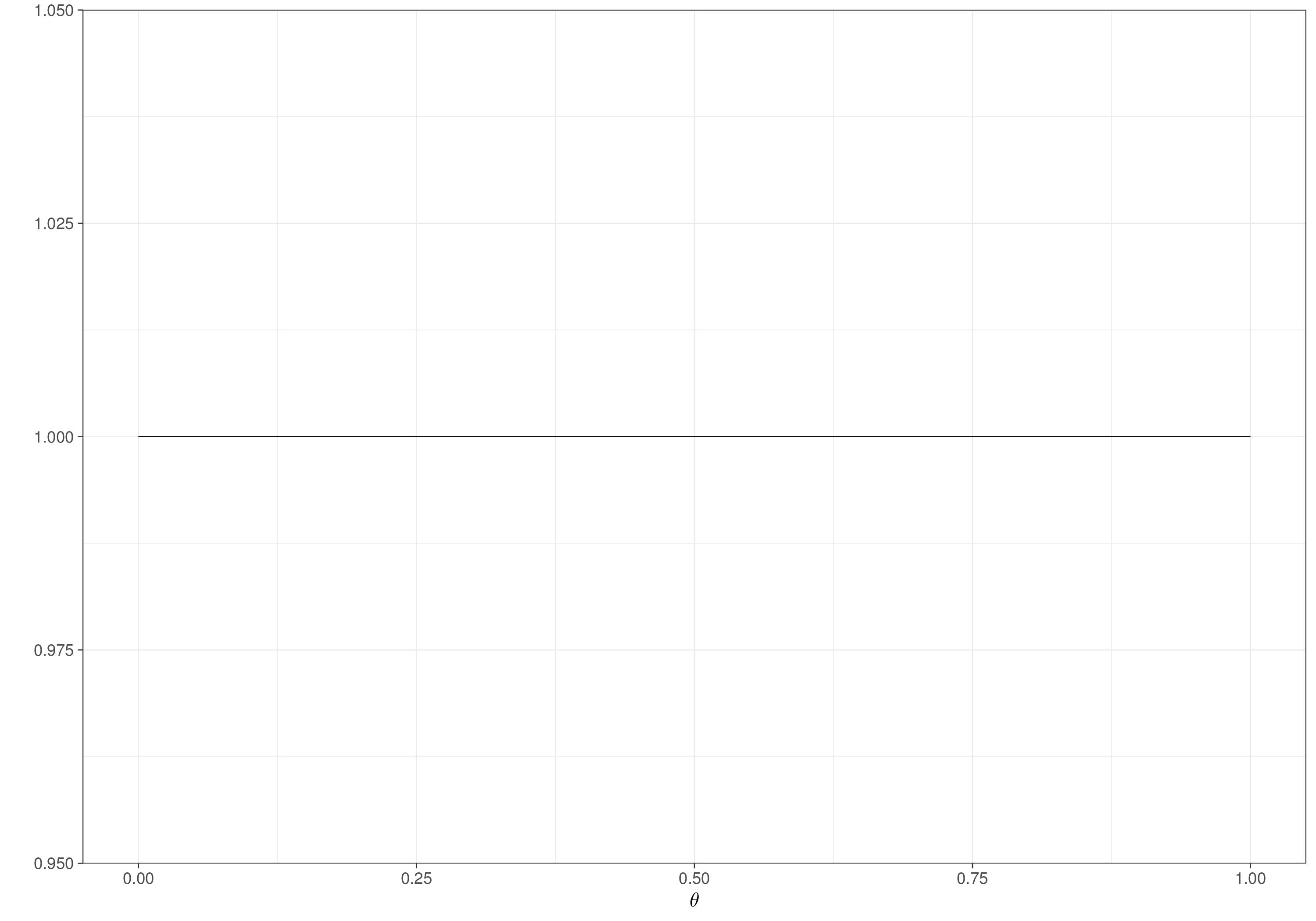
Example 2.1. Drug (continued): Uniform prior. The analysis of Example 1.5 can be replicated by changing the prior for \(\theta\) to a Uniform(0,1) distribution, using the following R code. This is fundamentally different from the Beta used before, as shown in Figure 2.1.
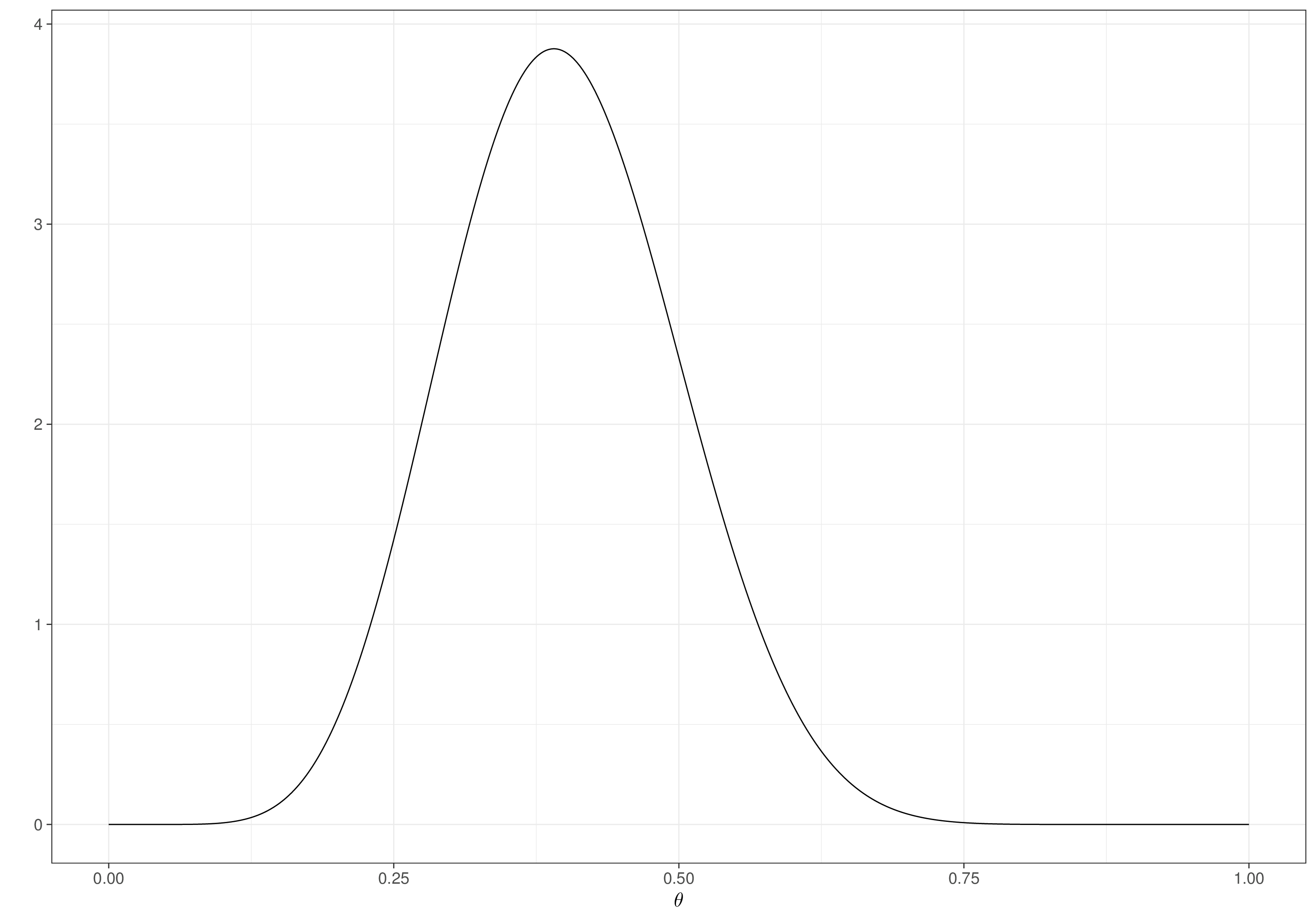
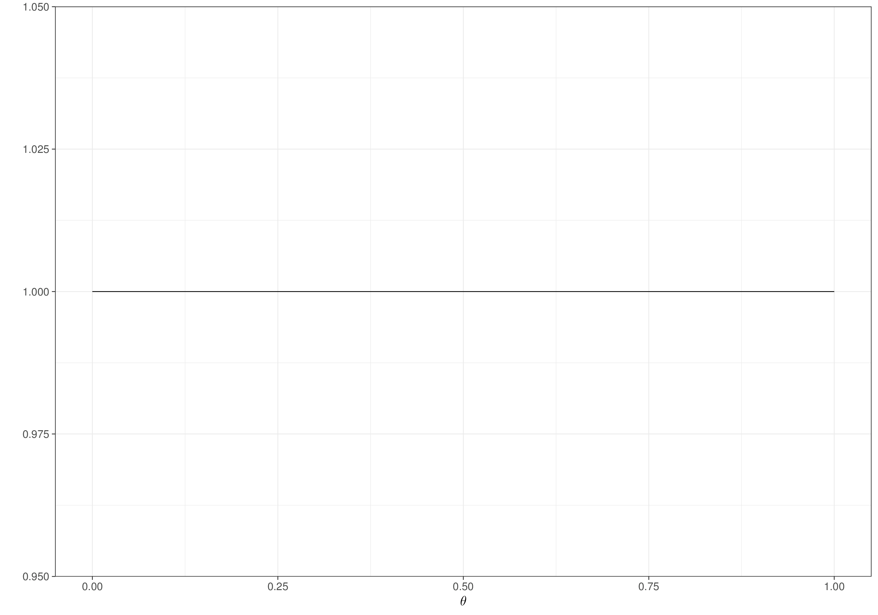
Visualising (different choices for) the prior distributions is always a good idea to understand what we are actually implying with the modelling assumptions we use. In this case, the Beta prior would be much more concentrated around the mean of 0.4, while the Uniform would imply a much larger range of plausible values. The latter may be considered as a “lazy” option – we can use it knowing that its natural range (the interval [0,1]) is reasonable for the underlying parameter (because \(\theta\) is a probability); but we are basically saying that we do not know anything whatsoever about the possibility that the drug is actually good. We most likely have much more information than this…
In any case, we can replicate the Monte Carlo analysis using both the Beta and the Uniform prior
# Simulates from the two priors for 'theta', Beta(9.2,13.8) and Uniform(0,1)
theta1=rbeta(n=nsim,shape1=9.2,shape2=13.8)
theta2=runif(n=nsim, min=0, max=1)

# MC (forward sampling) simulations of future data 'y1' and 'y2'
y1=rbinom(n=nsim,size=20,prob=theta1)
y2=rbinom(n=nsim,size=20,prob=theta2)
and then summarise the resulting distributions for \(y_1\) and \(y_2\) to see what effect the choice of the prior has had.
sims = cbind(y1,y2)
bmhe::stats(sims)
mean sd 2.5% median 97.5%
y1 8.0073 2.919949 3 8 14
y2 9.9092 6.063549 0 10 20The most striking result is that the second set of simulations show a much larger variance (and the 95% interval is between 0 and 20 – basically saying that it is very possible that every possible outcome can happen, in the trial, if we actually get money to run it…).
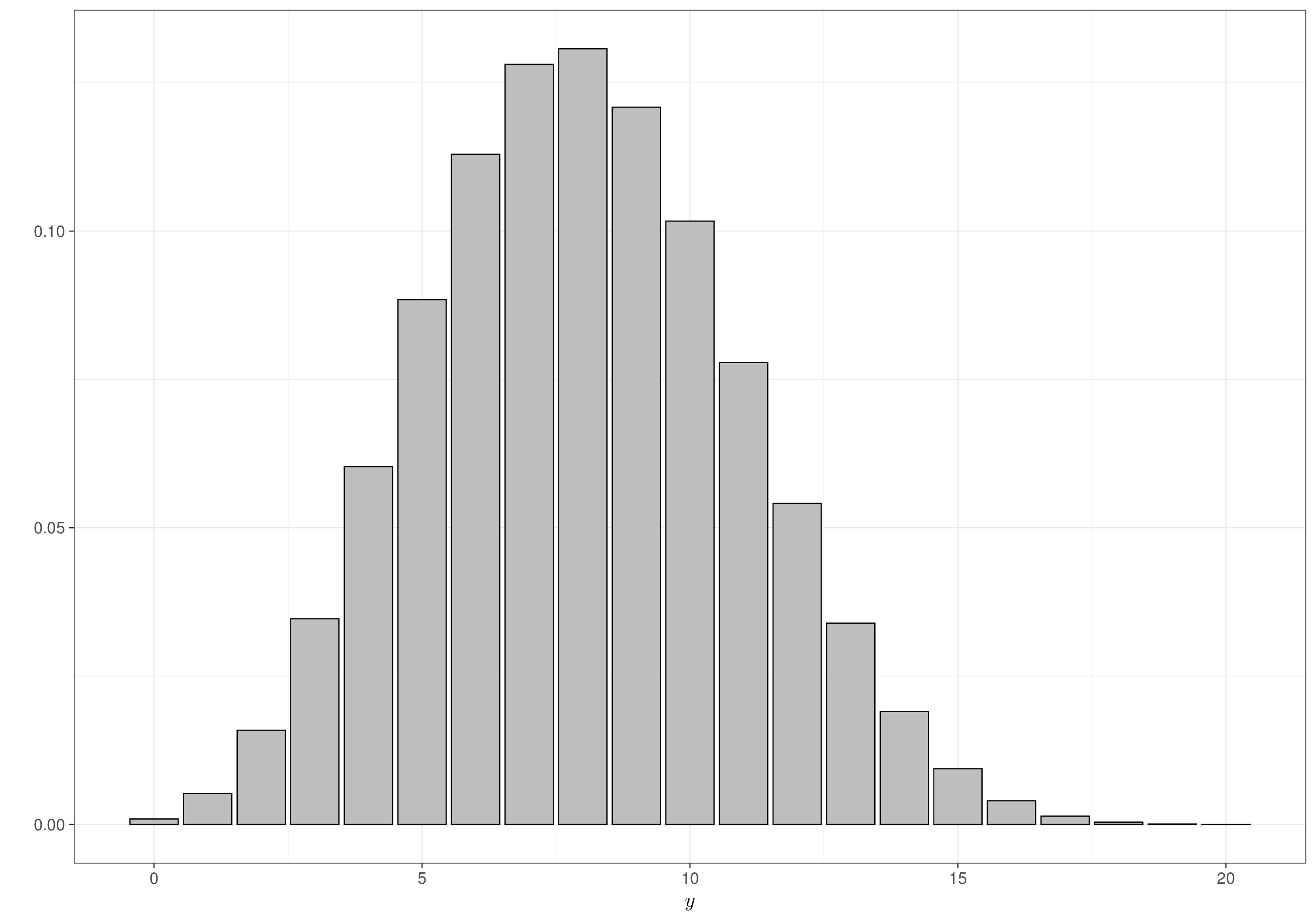
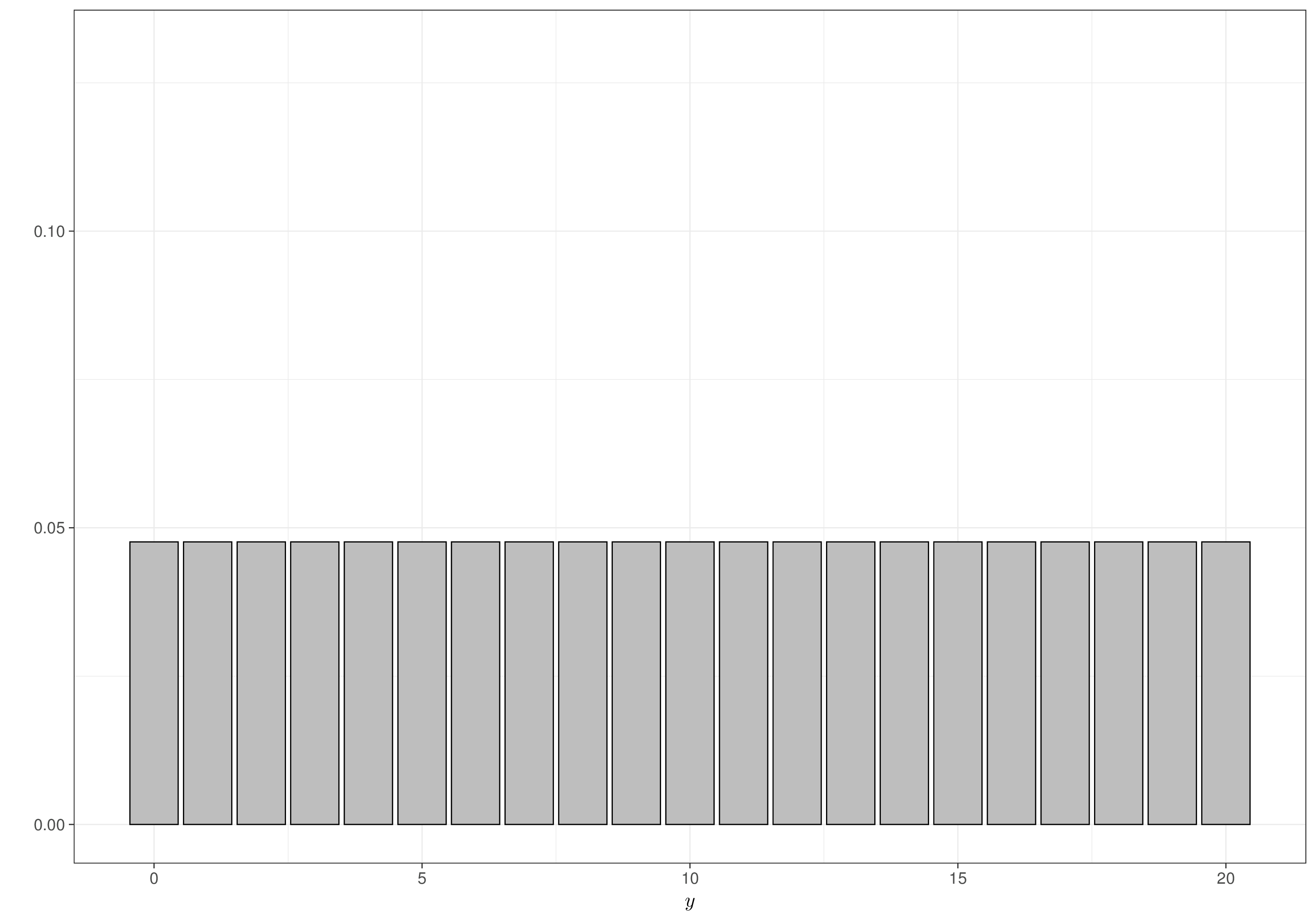
Figure 2.2 shows the resulting prior predictive distributions \(\displaystyle p(y)=\int p(y\mid\theta)p(\theta)d\theta\) (see Equation 1.7) for the two choices of priors. While both panels closely resemble the graphs in Figure 2.1, notice that the range along the \(x\)–axis is fundamentally different, as the priors are about the parameter \(\theta\) (which is defined between 0 and 1), while the predictive distributions are about possible future data (which are defined in the range 0 to 20, indicating that none or all of the potential \(n=20\) individuals have a successful outcome from using the drug). In addition, the graphs in Figure 2.1 show the two densities for the continuous variable \(\theta\), while those in Figure 2.2 display the probability distributions for the discrete variable \(y\). Figure 2.2 (a) is identical to Figure 1.13, as it represents the exact same analysis.
The advantage of using a Uniform prior is that we can directly perform posterior inference, in the face of actually observed data, with no computational expense. For example, suppose now that we manage to run a pilot study in which we select \(n=20\) patients from a relevant population and give them the drug. Out of these, \(y=15\) are fully relieved from their back pain.
By removing all the terms that do not depend directly on \(\theta\) from the Binomial sampling distribution of Equation 1.16 we obtain the likelihood function for this model as \[\mathcal{L}(\theta\mid y) = \theta^y \; (1-\theta)^{n -y}. \tag{2.3}\] Combining Equation 2.2 (which implies that, using a Uniform prior, the posterior is proportional to the likelihood) with Equation 2.3, we can conclude that \[ p(\theta\mid y,n) \propto \mathcal{L}(\theta\mid y,n) = \theta^{y} (1-\theta)^{n-y}, \] which is proportional to the kernel of the density for the Beta distribution shown in Equation 1.11. This in turn implies that \(\theta\mid y,n \sim \text{Beta}(y+1,n-y+1)=\text{Beta}(16,6)\) – we return to this point in Section 2.2.2 and Example 2.3.
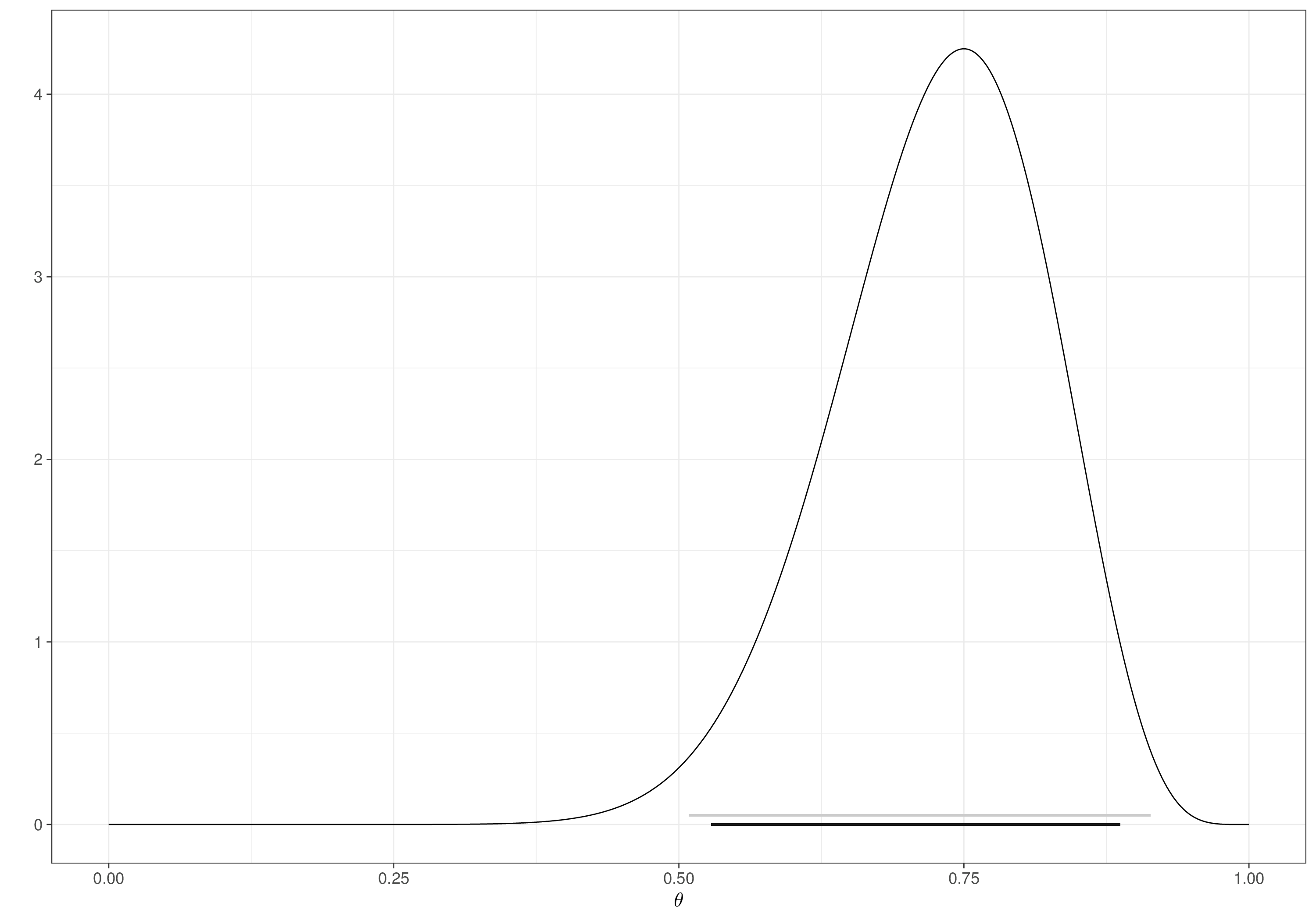
Figure 2.3 shows a graphical representation of this posterior distribution. The observation of the data effectively drives almost exclusively the inference – we can use Monte Carlo simulations to obtain a sample of observations from the posterior using the following R code and then bmhe to summarise the results, which are extremely similar to a maximum likelihood analysis, in which the MLE is \(\hat\theta=15/20=0.75\), with a confidence interval of \([0.509;0.913]\) – these numbers can be easily obtained using the R command binom.test(x=15,n=20).
# Sample from the posterior distribution
post=rbeta(10000,15+1,20-15+1)
# Use 'bmhe' to summarise the results
bmhe::stats(post)
mean sd 2.5% median 97.5%
0.72861422 0.09275955 0.52952955 0.73462481 0.88929082 Uniform priors also give us an alternative way of eliciting contextual knowledge and mapping it into suitable distributional assumptions (see Section 1.2.2). We can achieve this by performing a “pretend”, thought experiment to derive a suitable current level of uncertainty that we are willing to use in the prior.
The main idea is to think in terms of the alleged DGP and use an “implicit” dataset to update a state of absolute ignorance to a state of (possibly still substantial) uncertainty on the model parameters. In other words, we can start by assuming a “vague” prior to represent the (almost non-existing) background information and construct a model to tune the amount of data we would need to actually observe to modify this prior into a “posterior” that would match a state of uncertainty that we would be comfortable assuming. This updated distribution could then be used as a valid prior before observing any real data.
Example 2.2. Drug (continued): deriving contextual information via pseudo-data. Consider again Example 1.4, when we still have not made any observation \(y\) on the number of individuals who recover when given the drug, out of the \(n\) that we observe. We want to set up a prior distribution \(p(\theta)\) to describe our current uncertainty on the model parameter, which represents the probability that a random individual given the drug is relieved by their back-pain.
Let us assume that, to start with, we have no real information about the drug’s effectiveness, which we can represent by considering \(\theta\mid\mathcal{B}\sim\text{Uniform}(0,1)\) – exactly as in Laplace’s original analysis of Section 2.2.1 (notice here that we explicitly condition to the body of background knowledge, \(\mathcal{B}\)). We know from Equation 2.2 and the analysis in Example 2.1 that \(\theta\mid y_0,n_0 \sim \text{Beta}(y_0+1,n_0-y_0+1)\), with mean and variance \[\mu=\frac{y_0+1}{n_0+2} \quad\mbox{and}\quad \sigma^2=\frac{(y_0+1)(n_0-y_0+1)}{(n_0+2)^2(n_0+3)}\] (see Equation 1.12).
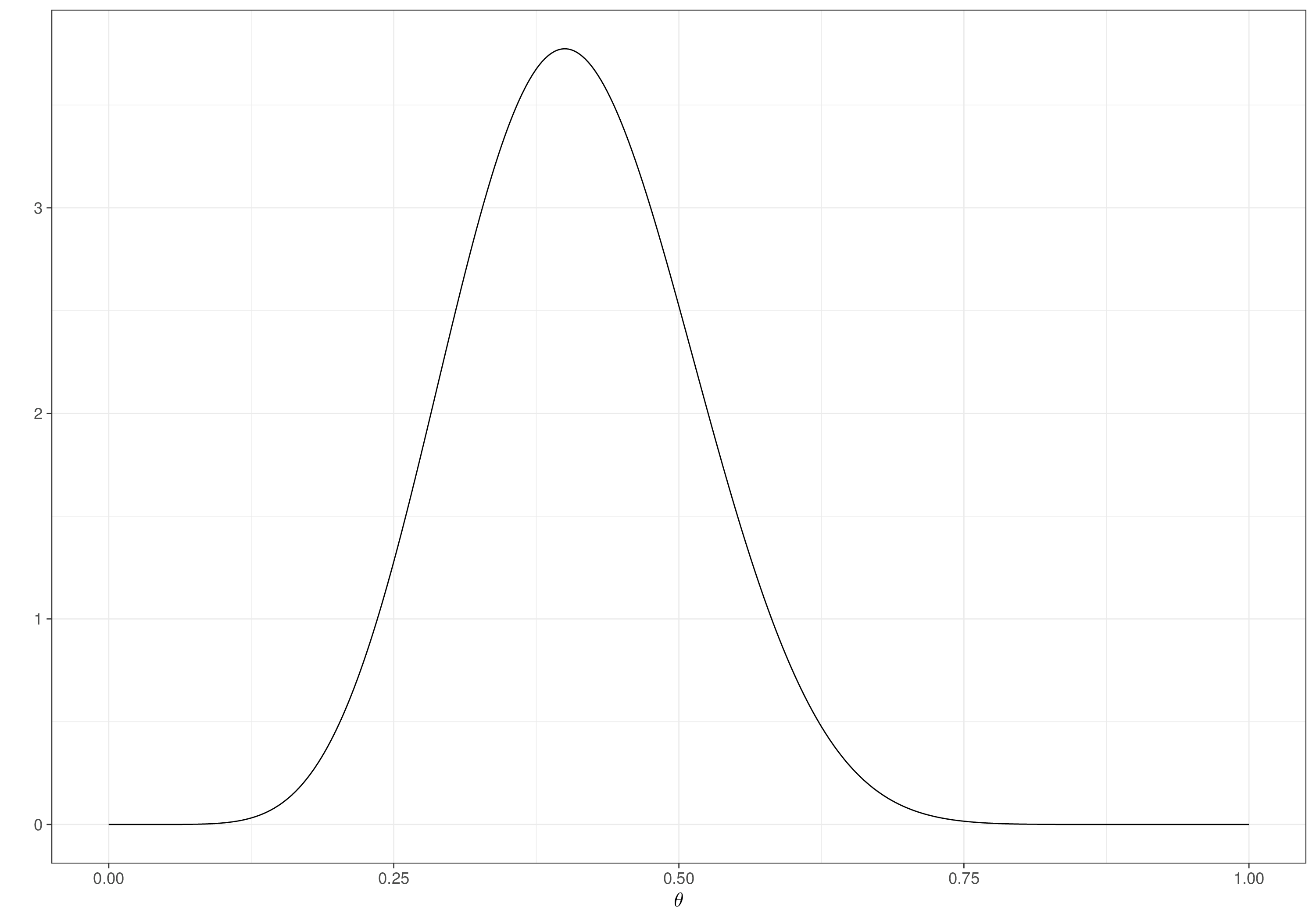
We can use trial-and-error and select different values for \((y_0,n_0)\) to calibrate our prior knowledge, as in Figure 2.4. For example, in Figure 2.4 (a) we elicit our prior knowledge in the form of a thought experiment in which we observe \(y_0=8\) successes, out of \(n_0=20\) individuals to whom we give the drug – as is possible to see, this pretty much amounts to the information that around 95% of the prior mass is included in \([0.2;0.6]\), with a mean of around 0.4 and a standard deviation of around 0.1, which we modelled using a \(\text{Beta}(9.2,13.8)\) in Example 1.4.
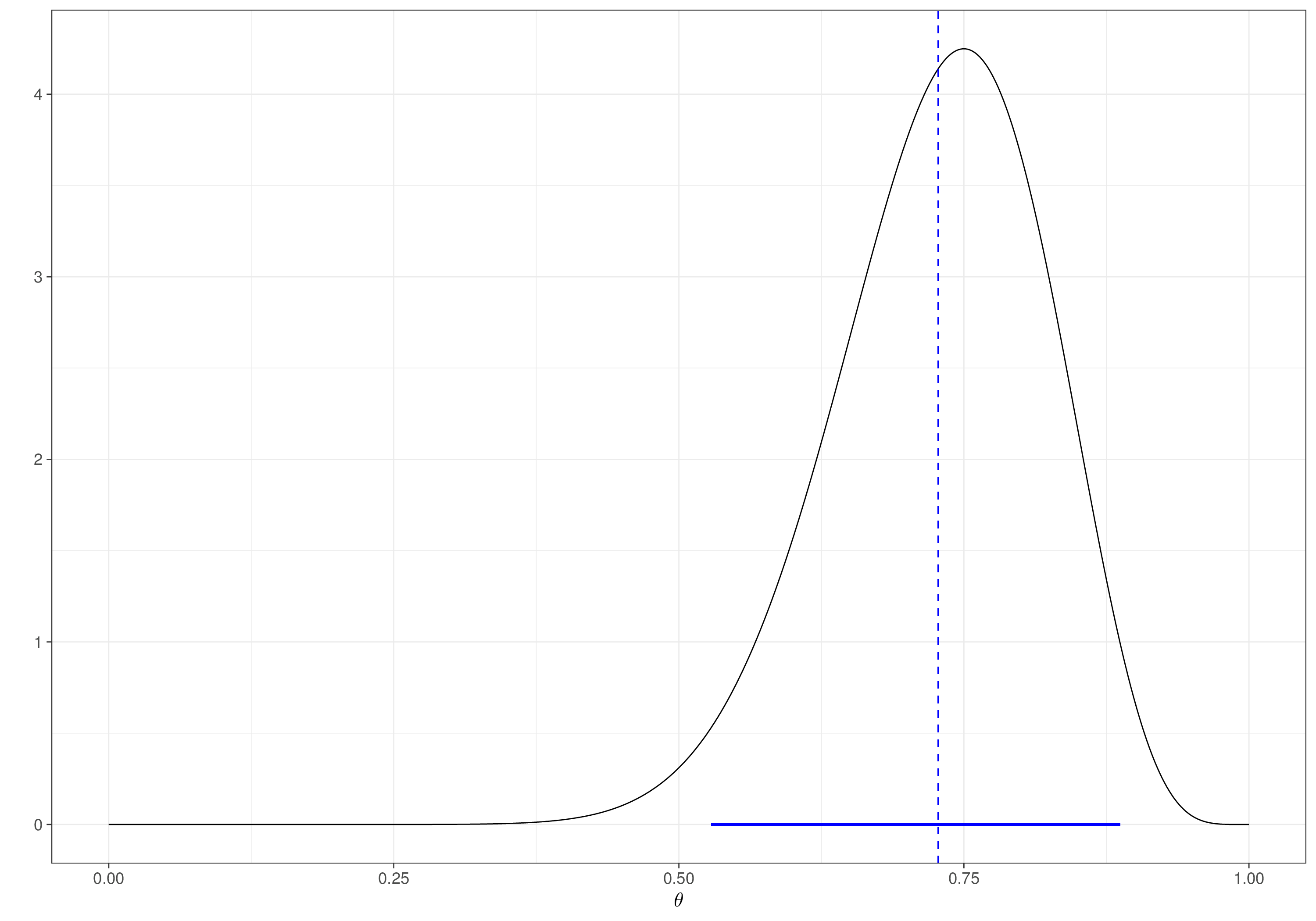
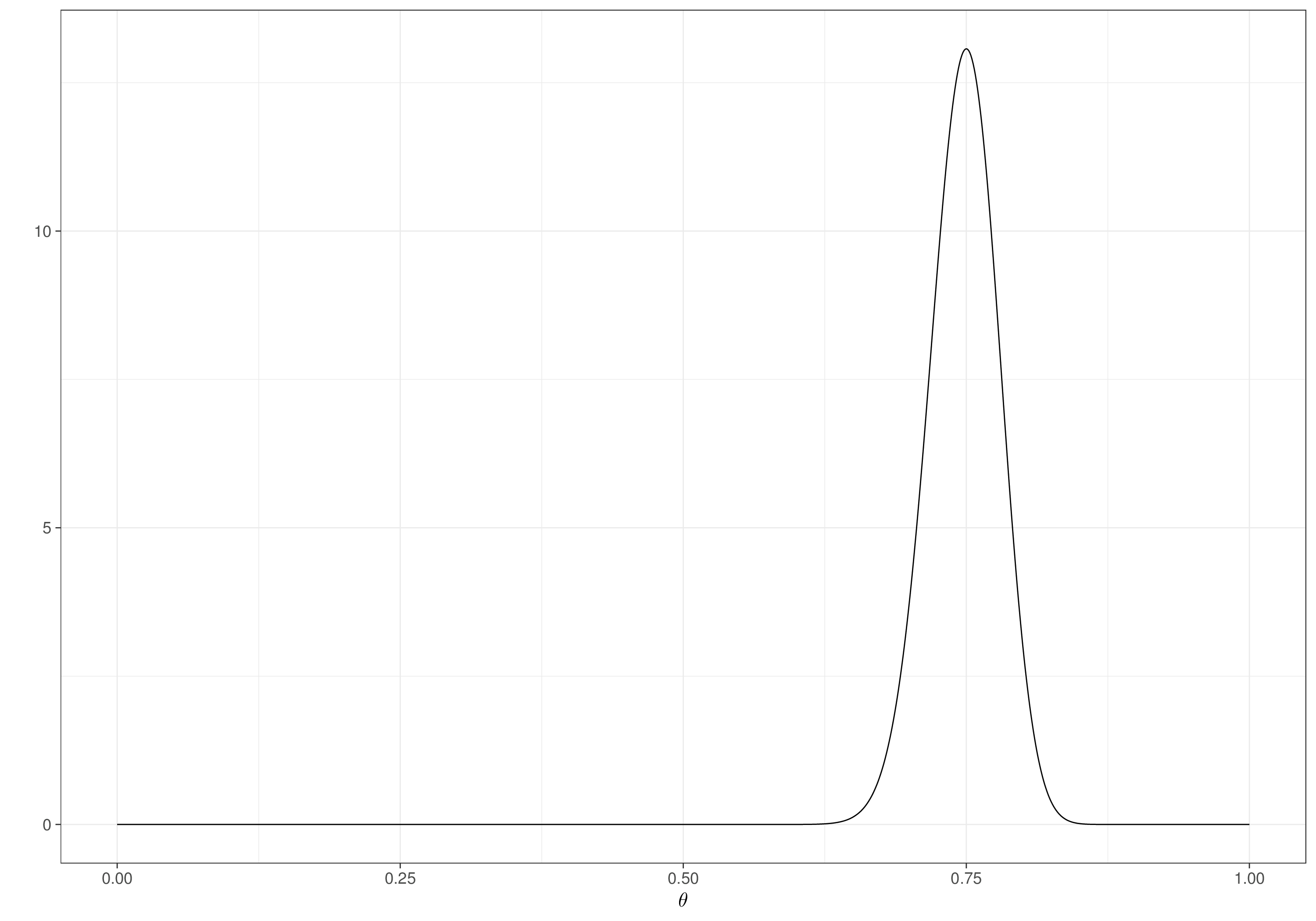
Figures 2.4 (b) and 2.4 (c) show two situations in which we are willing to assume that, on average, we expect a response rate of around 0.75 – the main difference is that in Figure 2.4 (b) we are not very confident about this possibility and thus we consider a “pretend” dataset with a very small sample size (\(n_0=20\)); in Figure 2.4 (c), while the sample proportion of successes is unchanged (\(150/200\) vs \(15/20\)), the sample size is ten times bigger, indicating that we would be much more confident with this assessment – we effectively would be basing it on a relatively large study in which around 75% of the individuals would have a positive outcome. As a result, the two densities are centred around the same value of 0.75, but the latter has a much smaller variance.
Finally, in Figure 2.4 (d) we show the case in which we elicit the prior information to amount to a study in which we pretend to have observed \(y_0=0\) successes, out of \(n_0=0\) trials. This obviously means that we assume we know nothing whatsoever on the drug’s effectiveness. Interestingly, when combined with the \(\text{Uniform}(0,1)\) prior we have assumed before even thinking of the thought experiment, implies a revised assessment that is still a \(\text{Uniform}(0,1)\). In fact, because we know that the posterior given \((y_0,n_0)\) is \(\text{Beta}(y_0+1,n_0-y_0+1)\), we can derive that \[\begin{eqnarray*} \text{Beta}(0+1,0-0+1) &= & \text{Beta}(1,1)=\frac{\Gamma(1+1)}{\Gamma(1)\Gamma(1)}\theta^{1-1}(1-\theta)^{1-1}\\ & = & 1=\frac{1}{1-0}=\text{Uniform}(0,1), \end{eqnarray*}\] recall from Equation 1.3 that \(\Gamma(x)=(x-1)!=(x-1)\times(x-2)\times\cdots\times 2\times 1\) and so \(\Gamma(1)=0!:=1\) and \(\Gamma(2)=1!:=1\). Thus, as is sensible, the thought experiment assuming \(y_0=n_0=0\) effectively implies “complete ignorance” and the non-informative prior.
While it is sometimes acceptable to imagine a near-complete lack of information in the possible range of likely values for the model parameters, this sort of assumption is often a “lazy” option. In reality, it is very difficult to justify a situation in which we are called to make inference on something about which we claim to know absolutely nothing.
In addition, the nature of the parameter for which we want to elicit a prior distribution may be such as to not conform very well with a Uniform distribution. Consider for example a regression model \[y_i \sim \text{Normal}(\mu_i,\sigma) \quad \mbox{with}\quad \mu_i=\beta_0 + \beta_1 x_i,\] for \(n\) observations \((y_i,x_i)_{i=1}^n\). A Bayesian formulation of this model requires setting prior distributions for the parameters \(\boldsymbol\theta=(\beta_0,\beta_1,\sigma)\).
We may not have (or may want to limit the impact of) any substantial contextual information and so aim at using vague priors. In line with the discussion above, we may spread the prior mass all over the range of the regression coefficients (so as not to favour any specific value) \[\beta_0,\beta_1 \stackrel{iid}{\sim} \text{Uniform}(-\infty,\infty).\] The problem here is that a Uniform distribution defined over the entire \(\mathbb{R}\) line has the inconvenient property of not integrating to 1, because \[\int_{\mathbb{R}} p(\beta_0)d\beta_0 = \int_{\mathbb{R}} cd\beta_0 = \int_{\mathbb{R}} p(\beta_1)d\beta_1= \int_{\mathbb{R}} cd\beta_1 \rightarrow \infty.\] This means that a Uniform prior over \(\mathbb{R}\) is not a proper probability distribution!
In some cases, it is still possible that the process of Bayesian updating transforms an improper prior into a proper posterior, i.e. \[\int_\Theta p(\theta\mid \boldsymbol{y})d\theta =1 \qquad \mbox{even if} \qquad \int_\Theta p(\theta)d\theta \rightarrow \infty,\] where \(\Theta\) is the range of the parameter \(\theta\). In general, however, improper priors are worrisome because a) their interpretation is meaningless, since they do not represent a probability distribution; and more importantly, b) the posterior may also remain improper, implying that the entire inferential process is meaningless.
For this reason, when the parameter of interest is unbounded, we may want to express “vagueness” using a different prior – a popular (and sensible) choice is to use a Normal distribution with large variance, i.e. \(\theta \sim\text{Normal}(0,s)\), for a large constant standard deviation, \(s\). Figure 2.5 shows such an example (with \(s=100000\)).
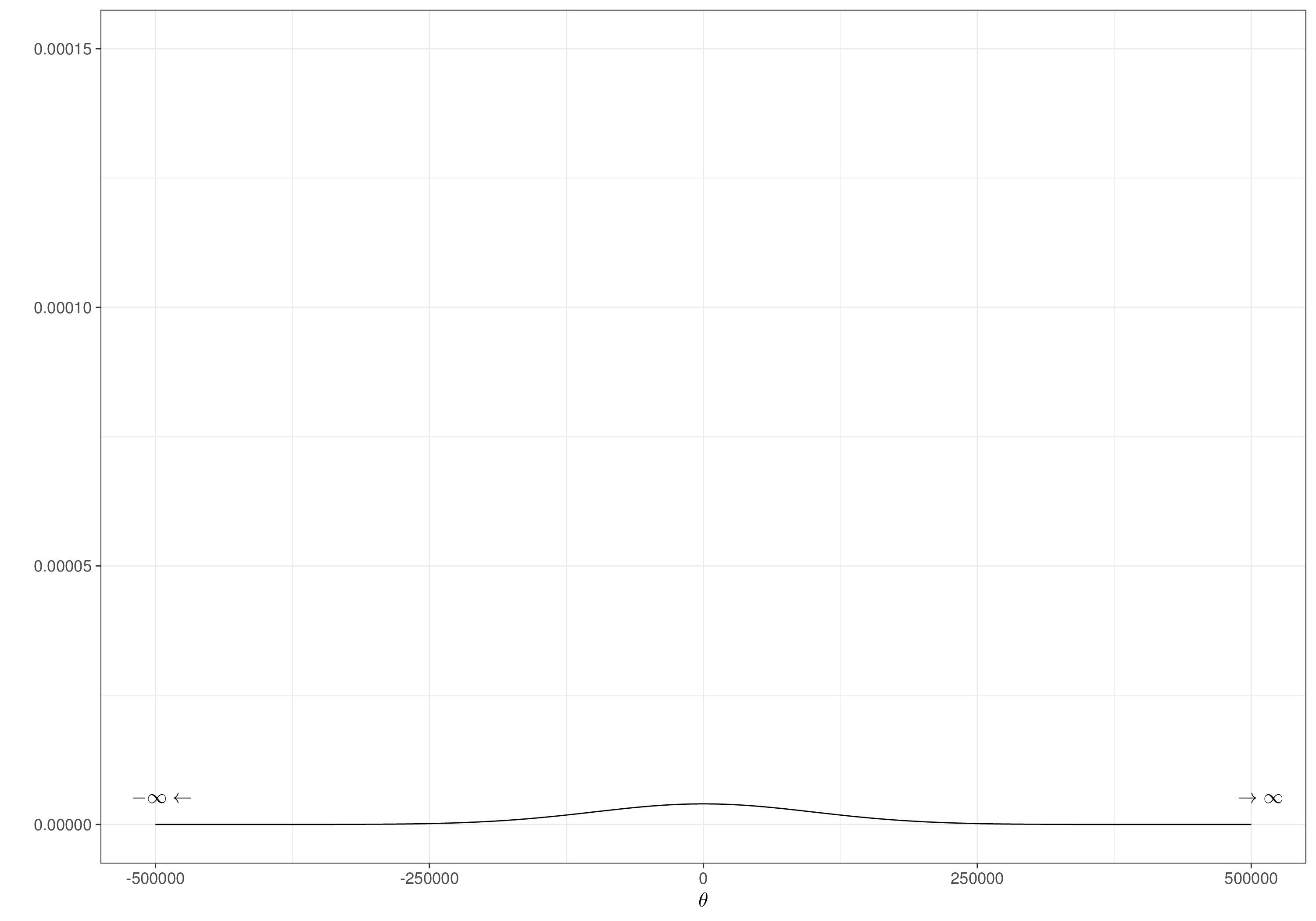
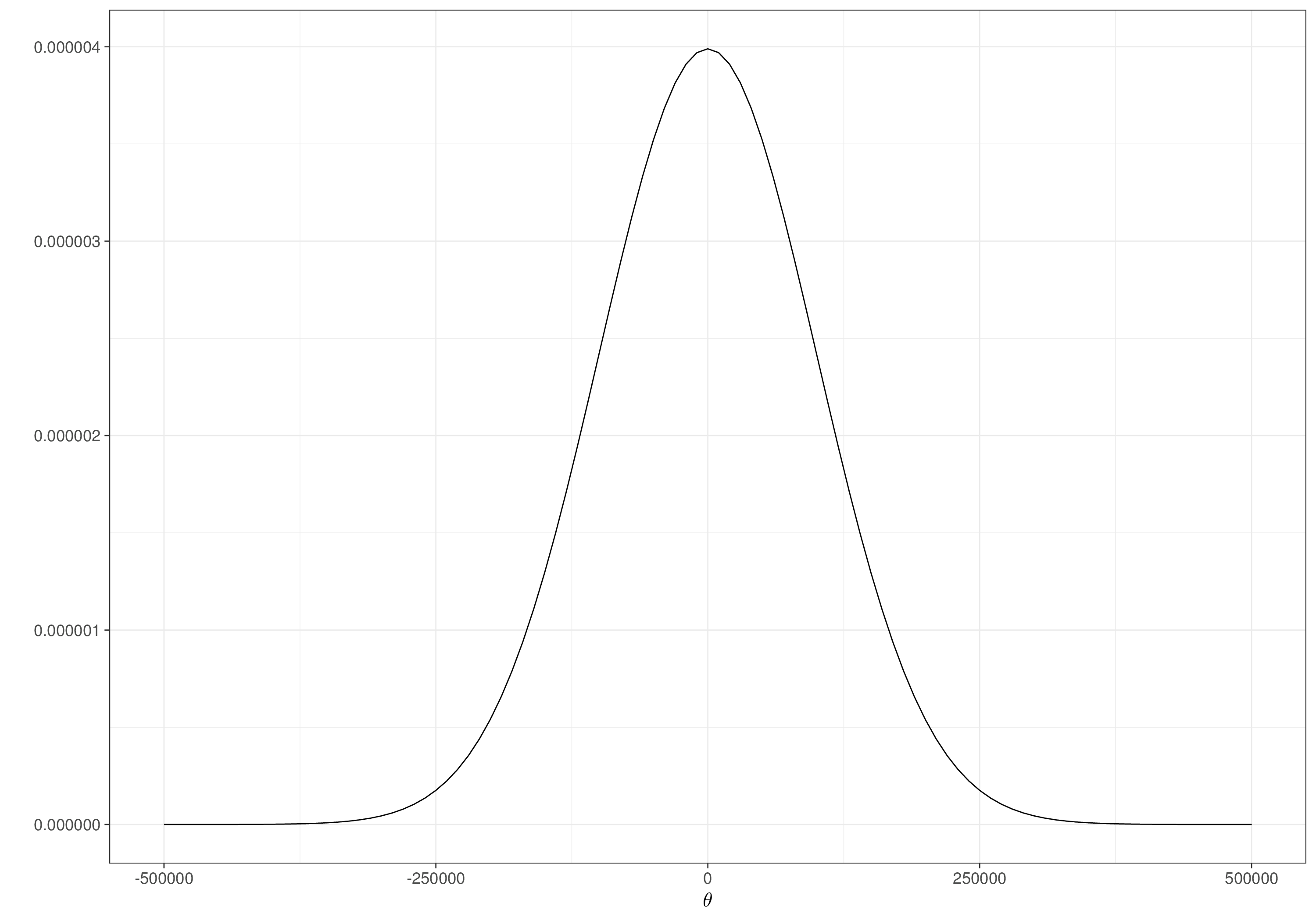
In some cases, it is not a major problem to use such extremely vague Normal priors, e.g. if we have enough data \((y_i,x_i)\) to fit our regression model, which means that the evidence in the likelihood will dominate in forming the posterior. But especially when data are sparse or non-definitive, “lazy” options such as these may lead to unnecessary inefficiencies, or even fundamental bias in our inference. In fact, in effectively every applied problem, we should be able to do better than just assuming that “anything goes”: odds ratios are hardly ever bigger than 3 or 4; the scale of a covariate effect can be determined with some level of approximation in a finite interval etc. – all these considerations can be used to determine a “large enough” value for \(s\), without going crazy about it…
NoteObjective subjectivity
From a purely Bayesian point of view, we would actually never want to limit the impact of contextual information. In fact, we would highlight its use as a defining feature of our analysis.
The idea of “hiding” the subjectivity inherent in a Bayesian modelling is more of a “historically accident” – at a time when frequentism was the dominant philosophical paradigm for probability (roughly speaking, for large part of the 20th century), Bayesians found themselves trying to defend their views by suggesting that subjectivism could be limited by taking appropriate actions in forming the prior, e.g. using vague (or “non-informative”) distributions – see also Note 2.1 below.
At the same time, prominent Bayesian scholars such as Dennis Lindley, Bruno de Finetti and Leonard Jimmie Savage were adamant that subjectivism was a key feature of science and continued to advocate for a “proper” use of the Bayesian machinery in statistical inference, thus taking full stock of any contextual information, whenever available.
2.2.2 Conjugate analysis
Until the mid-1990s, when simulation algorithms adapted from Physics (see Section 2.3 and Section 2.3.1) effectively rendered Bayesian computation feasible for problems of, virtually, any level of complexity, a “conjugate analysis” was the only practical way of running Bayesian modelling.
The main ideas originated in the Bayesian school at the University of Chicago, in the US, with the work of Raiffa and Schlaifer (1961) and build on the recognition that, sometimes, it is possible to exploit the mathematical form of a given prior distribution, which, when combined with the likelihood corresponding to a particular sampling distribution for the data, has the very convenient property that the resulting posterior distribution remains in the same parametric family as the prior.
Technically, a prior distribution \(p(\theta)\) is said to be “conjugate” to a given likelihood if \[p(\theta) \in f(\theta; \boldsymbol{a}) \quad\Rightarrow\quad p(\theta\mid y) \propto p(\theta)\mathcal{L}(\theta\mid y) \in f(\theta; \boldsymbol{a^*}), \tag{2.4}\] where \(f(\theta; \boldsymbol{a})\) is a parametric family (e.g. a Beta, or a Gamma), as a function of a set of parameters \(\boldsymbol{a}\), e.g. \((a,b)\) in Equation 1.11. Equation 2.4 implies that, under conjugacy, the posterior distribution belongs to the same distributional family as the prior, \(f(\cdot)\) – the update only involves the parameters that change from \(\boldsymbol{a}\) to \(\boldsymbol{a^*}\), by effect of the information contained in the likelihood function.
NoteSufficient statistics and conjugacy
If a sufficient statistic \(S(y)\) of fixed dimension exists for a given likelihood function \(\mathcal{L}(\theta\mid y)\), then any arbitrarily large data can be summarised fully through it – technically, this can be represented equivalently using either of the following relationships \[ p(y\mid S(y),\theta)=p(y\mid S(y)) \Leftrightarrow y \perp\!\!\!\perp \theta \mid S(y), \] which also hold when we can express the sampling distribution as \[p(y\mid \theta)=h(y)g(S(y),\theta), \tag{2.5}\] for given functions \(h(\cdot)\) and \(g(\cdot)\).
The sufficient statistic tells us everything we need to know about the parameter and thus, conditionally on it, the distribution of the data \(y\) is independent on the parameter \(\theta\) and, in particular, from Equation 2.5 we can see that the data only enter the likelihood through \(S(y)\).
Although this concept is grounded in Fisher’s likelihood theory (which also fulfills the most important frequentist principles – cfr. Note 1.1 in Section 1.1), it does play a key role in Bayesian modelling too, because if a sufficient statistic exists for a given model, then we can prove that a conjugate prior distribution also exists (Raiffa and Schlaifer, 1961; DeGroot, 1970).
Consider for example a sample of \(n\) independent observations \(\boldsymbol{y}=(y_1,\ldots,y_n)\sim\text{Normal}(\mu,\sigma)\), for some fixed value2 \(\sigma\). The multivariate form of the sampling distribution is \[p(\boldsymbol{y}\mid \mu,\sigma)=\left(\frac{1}{2\pi\sigma^2}\right)^{\frac{n}{2}}\exp\left(-\frac{1}{2\sigma^2}\sum_{i=1}^n\left(y_i - \mu\right)^2\right).\] If we use some simple algebra to re-write \[\sum_{i=1}^n\left(y_i -\mu\right)^2 = n(\mu-\bar{y})^2 + \sum_{i=1}^n\left(y_i-\bar{y}\right)^2,\] then we can rearrange the sampling distribution as \[p(\boldsymbol{y}\mid \mu,\sigma)=\left(\frac{1}{2\pi\sigma^2}\right)^{\frac{n}{2}}\exp\left(-\frac{1}{2\sigma^2}\sum_{i=1}^n\left(y_i-\bar{y}\right)^2\right) \exp\left(-\frac{n}{2\sigma^2}\left(\mu-\bar{y}\right)^2\right). \tag{2.6}\]
The only term in Equation 2.6 that is a function of \(\mu\), i.e. the likelihood function for the parameter of interest \(\mu\), given the observed data \(\boldsymbol{y}\) and the “nuisance” parameter \(\sigma\), is then \[\mathcal{L}(\mu\mid\boldsymbol{y},\sigma)=\exp\left(-\frac{n}{2\sigma^2}\left(\mu-\bar{y}\right)^2\right), \tag{2.7}\] which depends on the observed data only through the sample mean \(\bar{y}\) and the sample size \(n\) – which are thus the two sufficient statistics: all the information contained in the data can be summarised fully through \(\boldsymbol{S}=(\bar{y},n)\).
Interestingly, as a function of \(\mu\), Equation 2.7 closely resembles the kernel of a Normal density (see Equation 1.4) and the intuition behind conjugacy is that, if we define a prior based on this form, i.e. in this case \(\mu\sim\text{Normal}(m_0,s_0)\) for some set values \(m_0,s_0\) for the mean and standard deviation, then we can compute the posterior distribution as \[ \begin{aligned} p(\mu\mid\boldsymbol{y},\sigma) & \propto p(\mu\mid m_0,s_0)\mathcal{L}(\mu\mid\boldsymbol{y},\sigma) \\ & \propto \exp\left(-\frac{1}{2s_0^2}\left(\mu-m_0\right)^2\right) \exp\left(-\frac{n}{2\sigma^2}\left(\mu-\bar{y}\right)^2\right), \end{aligned} \] which, with some simple algebra, we can re-write as \[ \exp\left(-\frac{1}{2}\left(\frac{1}{s^2_0}+\frac{1}{\sigma^2}\right)\left(\mu -\left(\frac{1}{s^2_0}+\frac{1}{\sigma^2}\right)^{-1}\left(\frac{m_0}{s^2_0}+\frac{n\bar{y}}{\sigma^2}\right)\right)^2\right). \]
This is in turn again the kernel of a Normal density, meaning that the posterior remains in the same parametric family as the prior and is \(\mu\mid \boldsymbol{y} \sim \text{Normal}(m_1,s_1)\), with \[ m_1 = s^2_1\left(\frac{m_0}{s_0^2} + \frac{n\bar{y}}{\sigma^2}\right) \quad\mbox{and}\quad s_1=\sqrt{\left(\frac{1}{s^2_0}+\frac{n}{\sigma^2}\right)^{-1}}. \tag{2.8}\]
A large number of conjugate models exist for set inferential problems (cfr. Table 3.1 in Lunn et al., 2013 for a list of univariate conjugate models). Examples include \[ \left\{ \begin{array}{l} \theta \sim \text{Gamma}(a,b) \\ y_1,\ldots,y_n\mid\theta \stackrel{iid}{\sim} \text{Poisson}(\theta) \end{array} \right. \quad \Rightarrow \quad \theta\mid \boldsymbol{y} \sim \text{Gamma}\left(a+\sum_{i=1}^n y_i, n+b\right) \] and \[ \left\{ \begin{array}{l} \displaystyle\tau = \frac{1}{\sigma^2} \sim \text{Gamma}(a,b) \\ y_1,\ldots,y_n\mid\mu,\sigma \stackrel{iid}{\sim} \text{Normal}(\mu,\sigma) \end{array} \right. \Rightarrow \tau \mid\mu,\boldsymbol{y} \sim \text{Gamma}\left(a+\frac{n}{2}, b+\frac{1}{2}\sum_{i=1}^n(y_i-\mu)^2\right) \tag{2.9}\] (note that Equation 2.9 is a posterior distribution considering \(\mu\) as fixed – see Example 2.7).
Example 2.3. Drug (continued): conjugate analysis. If we now model \(\theta\sim\text{Beta}(a_0,b_0)\) – say, again, with \(a_0=9.2\) and \(b_0=13.8\), given the form of the density for the Beta distribution shown in Equation 1.11, we can write \[ p(\theta\mid a_0,b_0)\propto \theta^{a_0-1}(1-\theta)^{b_0-1} \] and applying Bayes’ theorem, we obtain that \[\begin{eqnarray*} p(\theta\mid y) & \propto & p(\theta)\mathcal{L}(\theta\mid y) \\ & \propto & \theta^{a_0-1}(1-\theta)^{b_0-1} \theta^y \; (1-\theta)^{n -y} \\ & \propto & \theta^{a_0+y-1} (1-\theta)^{b_0+n-y-1} \\ & \propto & \theta^{a_1-1} (1-\theta)^{b_1 -1} \sim \text{Beta}(a_1,b_1), \end{eqnarray*}\] with \(a_1=a_0+y\) and \(b_1=b_0+n-y\), for the observed \(y=15\) and \(n=20\).
In other words, with these modelling assumptions, a Beta prior is updated to a Beta posterior by the observation of data whose sampling variability can be modelled using a Binomial distribution. The update does not involve the distributional form of the prior (which remains unchanged in the posterior), but only the parameters, which change from \((a_0,b_0)\) to \((a_1,b_1)\), as a function of the values for the observed data. This is obviously very attractive because we do not need any complex computational mechanism to obtain the posterior distribution in closed form.
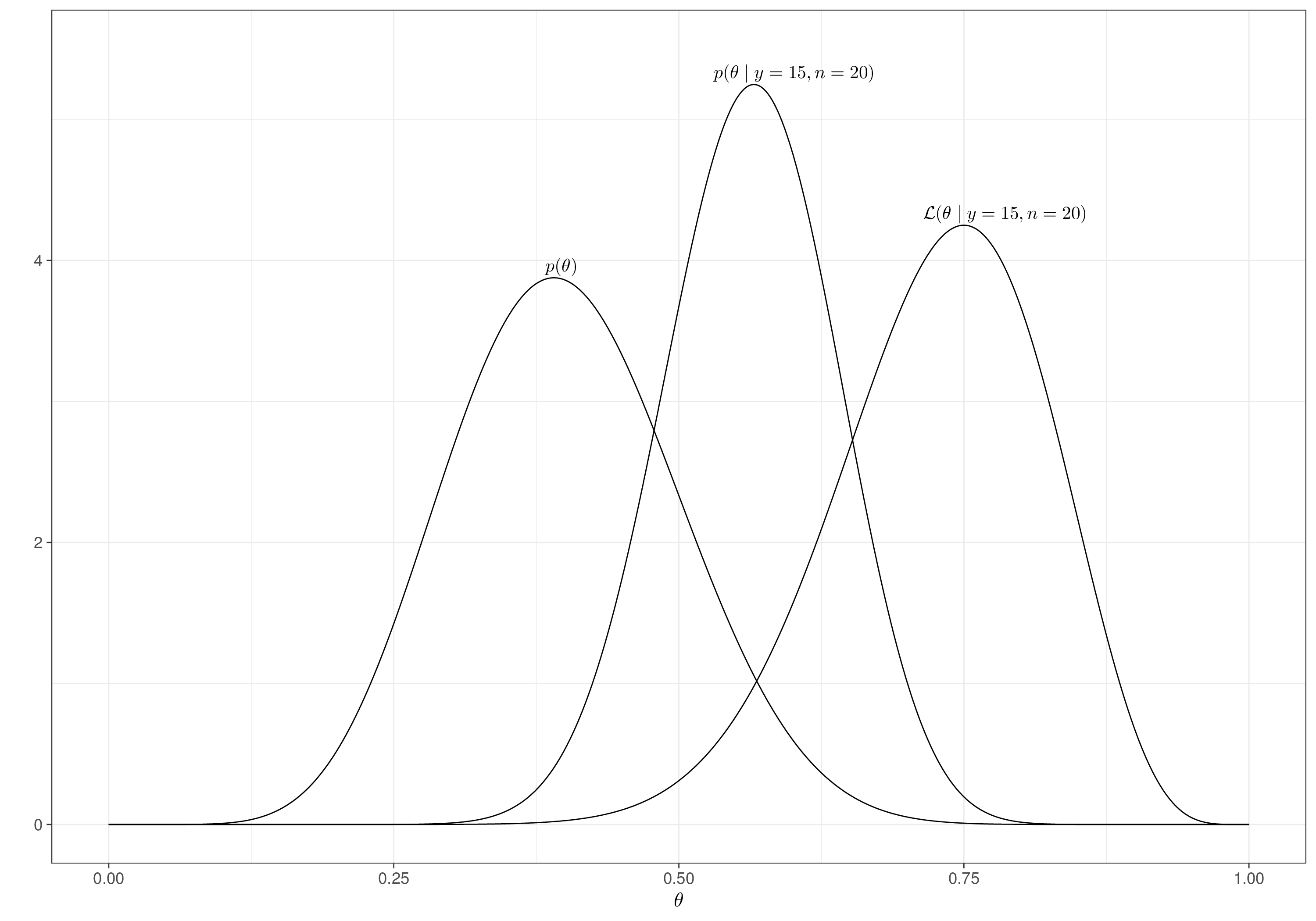
Figure 2.6 shows the prior, likelihood and resulting posterior using this conjugate analysis. In this case, the posterior results in a “compromise” between what we knew before observing the data and what we now know, after the data have become available. An analysis based on the likelihood function only would perhaps be overly-enthusiastic about the actual drug’s effectiveness – we do observe the vast majority of the patient to have a positive outcome.
Of course, it is possible that our prior be badly calibrated: perhaps the new drug is truly magical and thus the information available to us at the point of starting the experimentation bears little relevance and we should base our inference mostly on the data. Then again, generally speaking this surprising result is perhaps more likely to arise because of quirks in our data – perhaps the sample size is not large enough; or may be our patients are selected in a way that is not entirely representative of the underlying population, etc. For this reason, it makes sense, arguably, to include in our inference every little source of information we may have.
Conjugacy is a very handy property, from the mathematical perspective, but it can also be very restrictive, because it imposes a distributional form for the prior that may be insufficient to model the case at hand. For instance, there is no conjugated prior for a model such as logistic regression. Nevertheless, the computational appeal of conjugacy is sometimes still exploited even in real life, critical applications.
Example 2.4. Covid vaccine experimentation. In the wake of the Covid-19 pandemic, several biotechnology and pharmaceutical companies started collaborating on the development of a vaccine, in an unprecedented effort to deliver vital innovation in a short amount of time. The first vaccine to be approved by the US Food and Drug Administration (FDA, the federal agency responsible for ensuring safety of drugs introduced on the market, in the US) in December 2020 was the one developed jointly by German biotech company BioNTech and US pharmaceutical giant Pfizer. The development of the vaccine was based on a Phase I/II/III multicentre, placebo-controlled trial to evaluate the safety, tolerability, immunogenicity and efficacy of the candidate vaccine.
The Phase II/III study was designed using a Bayesian approach based on the following setup. There are two arms: one is randomised to receive two doses of a placebo, while the active arm receives two doses of the candidate vaccine. The data relevant for the efficacy analysis are the number of individuals who in each arm are confirmed Covid-19 cases, over the total number of individuals randomised to the specific arm. This can be formalised as \(y_{\textrm{plac}}\sim \text{Binomial}(\pi_{\textrm{plac}}, n_{\textrm{plac}})\) and \(y_{\textrm{vac}}\sim \text{Binomial}(\pi_{\textrm{vac}}, n_{\textrm{vac}})\), respectively. The actual measure of vaccine efficacy is defined as \(\mbox{VE}=\displaystyle\left(1-\frac{\pi_{\textrm{vac}}}{\pi_{\textrm{plac}}}\right)\), assuming a 1:1 allocation ratio in the two arms and thus \(n_{\textrm{plac}}=n_{\textrm{vac}}=N\).
However, the analysis is based on a reformulation of the problem: the experimenters actually model \(y=y_{\textrm{vac}}=\) number of Covid-19 cases among the individuals in the treatment arm over \(n=(y_{\textrm{vac}}+y_{\textrm{plac}})=\) the total number of Covid-19 cases in the two arms. This is modelled as \(y \sim \text{Binomial}(\theta,n)\), where \[\begin{eqnarray} \theta& = & \displaystyle\frac{\pi_{\textrm{vac}}}{\pi_{\textrm{vac}}+\pi_{\textrm{plac}}} \nonumber \\ & = & \frac{1-\mbox{VE}}{2-\mbox{VE}}. \end{eqnarray}\]
The reason for this seemingly overly-complex (and obscure) setup is that it allows the experimenters to only specify one observational model and, crucially, a single prior distribution for the parameter \(\theta\) – of course, once \(p(\theta\mid {\textrm{data}})\) is available, using the equation above, it is straightforward (e.g. through Monte Carlo simulation) to obtain directly the posterior distribution for the main parameter of interest \(p(\mbox{VE}\mid {\textrm{data}})\).
Sample size calculation
The determination of the sample size calculation is based on a simulation approach. The experimenter looked to determine a sample size large enough to be able to provide a probability exceeding 90% to conclude that \(\mbox{VE}>30\%\) with a “high probability” (we note here that the study protocol is vague on the actual threshold selected).
The simulation exercise proceeds in two steps. Firstly, the experimenters make assumptions about some of the features of the “data-generating process”. For instance, in the study protocol, they stipulate a “true” vaccine efficacy \(\widehat{\mbox{VE}} =0.6\) (i.e. a reduction by 40% in the infection rate in the vaccine arm, in comparison to the placebo population). This implies that the “true” proportion of Covid-19 cases in the vaccine arm over the total of cases is \[\hat\theta=\displaystyle\frac{1-\widehat{\mbox{VE}}}{2-\widehat{\mbox{VE}}}=0.2857.\]
Using these assumption, we can simulate a large number \(S\) (say, 100 000) of potential trial data from the alleged generating process \(y^{(s)}\sim \text{Binomial}(\hat\theta,n)\), where the superscript \((s)\) indicates the \(s\)–th simulated dataset and given a fixed value of the overall number of cases \(n\). Typically, we repeat the simulation for a grid of possible values of \(n\) (e.g. \(n=[10,20,30,40,50,60,70,\ldots]\)).
Once the hypothetical trial data have been generated, the second step consists in analysing them according to the statistical analysis plan defined in the protocol. In this case, the full model specification is required, which involves defining a prior distribution for \(\theta\).
For simplicity, the experimenters set a minimally informative Beta prior \(\theta \sim \text{Beta}(\alpha_0,\beta_0)\), where the parameters \(\alpha_0\) and \(\beta_0\) are selected to express the limited amount of information available a priori (recall that \(\theta\) represents the proportion of Covid-19 cases occurred in the vaccine group). We know from Equation 1.13 that \(\mbox{E}[\theta]=\displaystyle\frac{\alpha_0}{\alpha_0+\beta_0}\). If we fix \(\beta_0=1\), then we can solve for \(\alpha_0\) so that the prior mean for \(\theta\) is equal to some pre-specified value – in particular, the experimenters had chosen a threshold of \(\mbox{VE}=30\%\) as the minimum level of efficacy they were prepared to entertain. This value can be mapped to the scale of \(\theta\) as \(\displaystyle \frac{1-0.3}{2-0.3}=0.4117\) and thus solving \[\begin{eqnarray*} \frac{\alpha_0}{\alpha_0+1} = 0.4117 \end{eqnarray*}\] gives \(\alpha_0=0.700102\).
Because of conjugacy, for each simulated dataset we can easily update the Beta\((0.700102,1)\) prior to a Beta\((\alpha_1,\beta_1)\) posterior distribution for \(\theta\), where \(\alpha_1=0.700102+y^{(s)}\) and \(\beta_1=1+n-y^{(s)}\). Moreover, for each simulation \(s\), we can compute analytically any tail-area probability from \(p(\theta\mid{\textrm{data}})\). Once again, we are really interested in \(\Pr(\mbox{VE}>0.3\mid{\textrm{data}})\), but using the deterministic relationship linking VE to \(\theta\), we can re-express this as \[\begin{eqnarray*} \Pr(\mbox{VE}>0.3 \mid{\textrm{data}}) & = & \Pr\left(\frac{1-2\theta}{1-\theta}>0.3\mid{\textrm{data}}\right) \\ & = & \Pr(\theta<0.4117 \mid {\textrm{data}}), \end{eqnarray*}\] which can be computed for each simulation \(s\). This produces a large number of simulations that can be used to determine the “power” for a given sample size, as the proportion of times in which this computed probability exceeds a set threshold (i.e. is “large enough” in the phrasing of the study protocol).
The experimenters compute \(n=164\) as the optimal number of total Covid-19 cases that are necessary to be able to ascertain that \(\mbox{VE}>30\%\) with a large probability.
Then, it is necessary to determine the overall sample size (i.e. the total number of individuals to be recruited in the study) so that a total of 164 cases is likely to be observed within the required time frame. Once again, it is necessary to make some assumption about the data-generating process; specifically the experimenters consider a 1.3% illness rate per year in the placebo group. Because the study aims at accruing 164 cases within 6 months, this essentially amounts to assuming that \(\pi_{\textrm{plac}} \approx 0.013/2\) and thus \(\pi_{\textrm{vac}} \approx (\pi_{\textrm{plac}}\times 0.4)/2\) (recall that we are assuming a 60% vaccine efficacy, or that \(\pi_{\textrm{vac}}=0.4\times \pi_{\textrm{plac}}\)).
We can once again resort to simulations to estimate what sample size in each arm \(N\) is necessary so that we can expect \(y_{\textrm{vac}}+y_{\textrm{plac}}\geq 164\) – this returns an optimal sample size of \(N=17\,600\) per group. Finally, considering an attrition rate of 20% (indicating that such proportion of individuals would not generate an evaluable outcome could be observed), the experimenters inflate the sample size to obtain \(N^*=\displaystyle\frac{N}{0.8}=21\,999\) per group (or a total of \(43\,998\) individuals).
Data analysis
At the end of the actual study (Polack et al., 2020), there were \(y_{\textrm{vac}}=8\) and \(y_{\textrm{plac}}=162\) confirmed Covid-19 cases in the vaccine and the placebo group, respectively. These imply that \(y=8\) and \(n=(8+162)=170\). However, there is a slight extra complication: the setup describe above implies the assumption of 1:1 allocation (i.e. \(n_{\textrm{plac}}=n_{\textrm{vac}}\)) – this is crucial to ensure the simple deterministic relationship between VE and \(\theta\). In actual fact, the placebo group had a slightly higher number of individuals, by the time of the data analysis (there were 17,411 and 17,511 individuals with valid data in the vaccine and placebo group, respectively). Thus, we need to rescale the observed data, which can be done by considering \(y_{\textrm{vac}}^*=y_{\textrm{vac}}\displaystyle\frac{17\,461}{17\,411}=8.02297\) and \(y_{\textrm{plac}}^*=y_{\textrm{plac}}\displaystyle\frac{17\,461}{17\,511}=161.53743\), where \(17\,461 = \displaystyle\frac{17\,411+17\,511}{2}\) and thus \(y^*=8.02297\) and \(n^*=169.5604\).
These data can be used to update the prior distribution Beta\((0.700102,1)\) into a Beta\((8.723072,162.5374)\) posterior for \(\theta\). Finally, we can rescale this posterior to determine the relevant posterior distribution \(p(\mbox{VE}\mid {\textrm{data}})\), for instance using Monte Carlo to simulate a large number \(S\) of values \(\theta^{(s)}\sim \text{Beta}(8.723072,162.5374)\) and then computing \(\mbox{VE}^{(s)}=\displaystyle\frac{1-2\theta^{(s)}}{1-\theta^{(s)}}\) and then use these to characterise the uncertainty around the vaccine efficacy.
# Sets up the value for the parameters
alpha.0=0.700102
beta.0=1
# Observed data
y=c(8,162)
n=c(17411,17511)
# So needs to reproportion as if the treatment arms had the same
# sample size (to be in line with model assumptions!)
y=y*mean(n)/n
# Now can update the Beta prior with the observed data
alpha.1=alpha.0+y[1]
beta.1=beta.0+y[2]

# Monte Carlo analysis for theta and ve
theta=rbeta(100000,alpha.1,beta.1)
ve=(1-2*theta)/(1-theta)
In this case, the posterior distributions \(p(\theta\mid {\textrm{data}})\) and \(p(\mbox{VE}\mid {\textrm{data}})\) can be visualised in Figure 2.7.
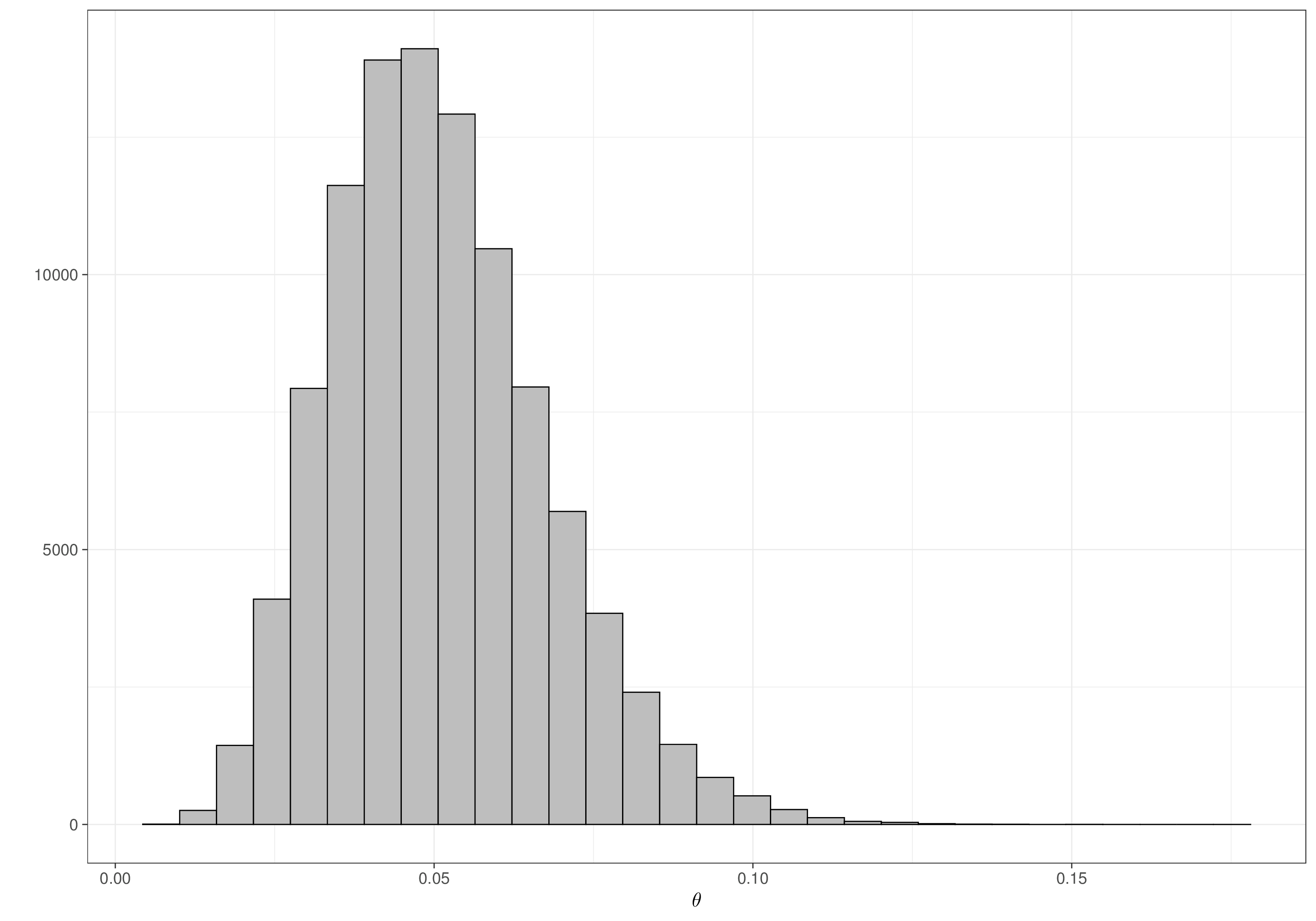
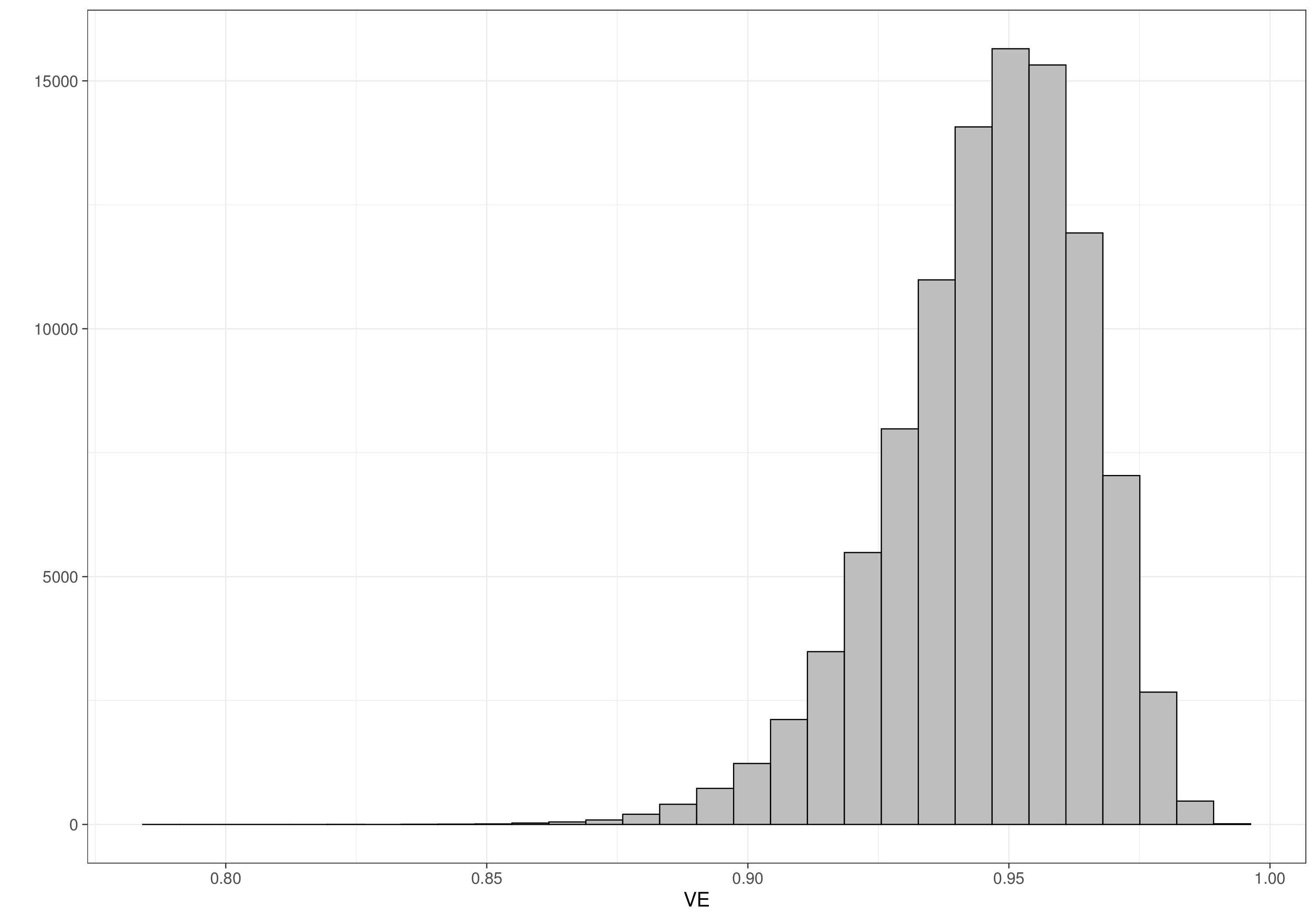
We can also use the resulting samples from the posterior distribution to estimate the 95% interval of \([0.9034; 0.9761]\) for the vaccine efficacy, indicating that we expect the vaccine to perform extremely well.
2.2.3 Penalised complexity priors
Simpson et al. (2017) have recently introduced the concept of “penalised complexity” (PC) prior. This is closely related to the principle of using “default” distributional assumptions and the basic idea is that PC priors can be constructed to penalise deviations from (i.e. added complexity in comparison to) the simpler, base model.
PC priors are based on four principles, underlying the features that Simpson et al. (2017) regard as desirable for a prior distribution in order for it to not influence the results unduly (i.e. over and above the impact of the data). The first principle is the philosophical idea of “Occam’s razor”, which suggests that modelling assumptions that are overlycomplicated should be discarded in favour of simpler ones, until there is enough support for the more complex version of the model.
The way in which “complexity” is measured in the framework of PC priors is through the Kullback-Leibler divergence (KLD), generically defined as \[\mbox{KLD}(f,g) = \int f(x)\log\left( \frac{f(x)}{g(x)} \right)dx,\] which is a measure of the information lost when some base model \(g\) is used as a possibly rough approximation to a more complex model \(f\), which includes some additional parameter \(\xi\).
A scaled version of the KLD, \(d(f,g)=\sqrt{2\mbox{KLD}(f,g)}\), is used as a measure of distance between two competing models. Assuming a constant rate of penalisation for increasingly complex models, essentially implies an Exponential distribution on the distance scale, \(d\): \(p(d) = \lambda \exp(-\lambda d)\sim\text{Exponential}(\lambda)\) – cfr Equation 1.10; also, this is akin to the consideration that the hazard is constant for an Exponential distribution, in survival modelling (see Chapter 8). Using the calculus rules for the change of support variable (see Equation 1.14), this corresponds to a prior on the parameter \(\xi\), which can be constructed in the form \[p(\xi) = \lambda e^{-\lambda d(\xi)}\left\lvert \frac{\partial d(\xi)}{\partial \xi} \right\rvert.\] Simpson et al. (2017) suggest that the parameter \(\lambda\) could be selected so as to control the prior mass in the tail of the resulting distribution for \(\xi\).
Example 2.5. PC prior for a standard deviation. Consider for example the two competing models for some data \(y\) as a function of a precision \(\tau=\sigma^{-2}\) \[g(\tau)\sim \text{Normal}(0,\tau=\tau_0\rightarrow \infty) \qquad \mbox{and} \qquad f(\tau)\sim \text{Normal}(0,\tau), \tau\in(0,\infty).\] This basically assumes that the “base case” model has \(\sigma=0\) (or equivalently \(\tau\rightarrow\infty\)) – see Chapter 6 for more applications of this concept in the context of hierarchical modelling.
If we parameterise the Normal distribution in Equation 1.4 with mean equal to 0 and in terms of the precision, we then get \[ f=\sqrt{\frac{\tau}{2\pi}}\exp\left(-\frac{\tau}{2}y^2\right) \quad \text{and} \quad g = \sqrt{\frac{\tau_0}{2\pi}}\exp\left(-\frac{\tau_0}{2}y^2\right). \] Thus \[ \begin{aligned} \text{KLD}(f,g) & =\int \text{Normal}(0,\tau) \left[\frac{1}{2}\log\left(\frac{\tau}{\tau_0}\right) - \frac{y^2}{2}\left(\tau-\tau_0\right)\right] dy \\ & = \frac{1}{2}\log\left(\frac{\tau}{\tau_0}\right)\underbrace{\int \text{Normal}(0,\tau)dy}_{=1} -\frac{1}{2}(\tau-\tau_0)\underbrace{\int y^2 \text{Normal}(0,\tau)dy}_{=1/\tau} \\ & = \frac{1}{2}\log\left(\frac{\tau}{\tau_0}\right) -\frac{1}{2}\frac{\tau-\tau_0}{\tau} \\ & = \frac{1}{2}\frac{\tau_0}{\tau}\left[1 + \frac{\tau}{\tau_0}\log\left(\frac{\tau}{\tau_0}\right) - \frac{\tau}{\tau_0}\right] \rightarrow \frac{1}{2}\frac{\tau_0}{\tau}, \end{aligned} \] because \(\tau_0\rightarrow \infty\). Thus \[ d(\tau)=\sqrt{2\mbox{KLD}(f,g)}=\sqrt{\frac{\tau_0}{\tau}}=\tau_0^{1/2}\tau^{-1/2}\propto \tau^{-1/2}. \]
Assuming \(p(d)=\lambda\exp(-\lambda d)\) then
\[\begin{eqnarray*} \left\lvert \frac{\partial d(\tau)}{\partial \tau} \right\rvert = \left\lvert -\frac{1}{2}\tau^{-3/2}\right\lvert = \frac{1}{2}\tau^{-3/2} \quad \Rightarrow \quad p(\tau) & \!\!= & \!\! \lambda\exp\left[-\lambda d(\tau)\right]\left\lvert \frac{\partial d(\tau)}{\partial \tau} \right\rvert \\ & \!\! = & \!\! \frac{\lambda}{2}\tau^{-3/2} \exp\left( -\lambda \tau^{-1/2}\right) \\ & \!\! \sim & \!\! \mbox{type-2 Gumbel}\left(a=\frac{1}{2},b=\lambda\right) \end{eqnarray*}\] and \[\begin{eqnarray*} \left\lvert\frac{\partial\tau}{\partial\sigma}\right\lvert=\left\lvert\frac{\partial\sigma^{-2}}{\partial\sigma}\right\lvert=\lvert -2\sigma^{-3}\lvert=2\sigma^{-3} \quad \Rightarrow \quad p(\sigma) & \!\! = & \!\! \frac{\lambda}{2}\sigma^3\exp\left(-\lambda\sigma\right)\left\lvert\frac{\partial\tau}{\partial\sigma}\right\lvert\\ & \!\! = & \!\! \lambda\exp(-\lambda\sigma)\sim\text{Exponential}(\lambda). \end{eqnarray*}\]
We can control the amount of information we include in the Exponential prior for \(\sigma\) by modulating the value of the parameter \(\lambda\). For example, we could set a constraint \(\Pr(\sigma>\sigma_0)=\alpha\), in terms of the constants \(\sigma_0\) and \(\alpha\), which by the properties of the Exponential distribution implies \[\lambda=-\frac{\log(\alpha)}{\sigma_0}.\]
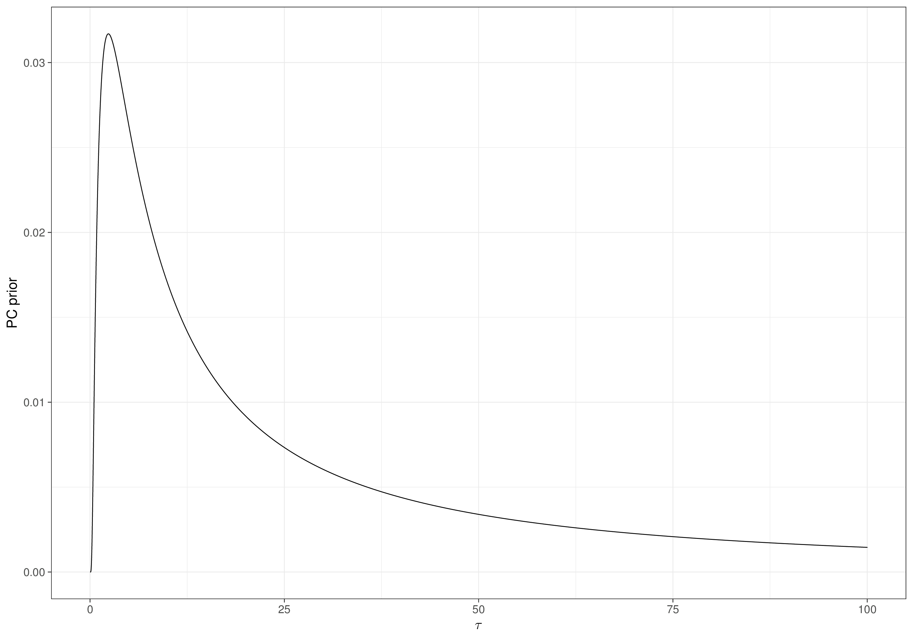
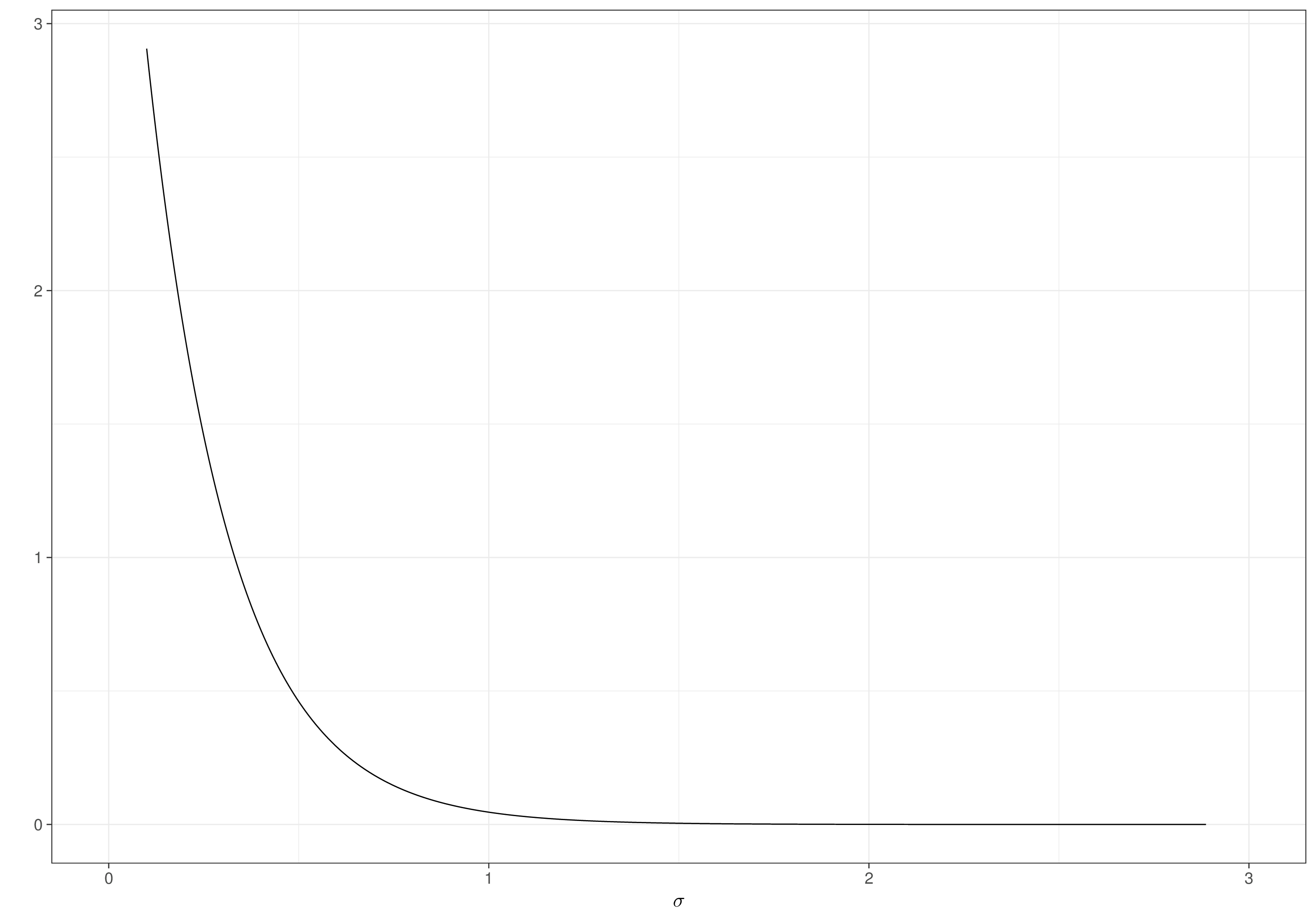
So, for instance, setting \(\alpha=0.01\) and \(\sigma_0=1\), we get \[\Pr(\sigma >1)=0.01 \Rightarrow \lambda = -\log(0.01) \approx 4.61\] and thus the resulting PC prior is \(\sigma \sim \text{Exponential}(4.61)\), which is depicted in Figure 2.8 (b), together with the prior on \(\tau\), in Figure 2.8 (a).
Note 2.1: Jeffreys’ default prior
The idea of using a “default” prior to limit the subjective element of a Bayesian analysis is not new – Jeffreys (1961) provides a comprehensive review of work originating as far back as the 1930s. Jeffreys’ work is grounded in the midst of the frequentist domination, when Bayesian modelling was seen as impractical as well as philosophically unsound, because of the subjectivity intrinsic in the analysis. To combat this, he proposed a prior of the form \[p(\theta)\propto \mathcal{I}(\theta)^{1/2},\] where \[\mathcal{I}(\theta)=-\mbox{E}_{Y\mid\theta}\left[\frac{\partial^2\log \mathcal{L}(\theta\mid y)}{\partial\theta^2}\right] = \mbox{E}_{Y\mid\theta}\left[\left(\frac{\partial\log \mathcal{L}(\theta\mid y)}{\partial\theta}\right)^2\right]\] is the , a measure of the amount of information that the observable random quantity \(y\) carries on the parameter \(\theta\).
For example, the likelihood associated with \(y\sim\text{Binomial}(\theta,n)\) is as in Equation 2.3; thus \[ \frac{\partial\log \mathcal{L}(\theta\mid y)}{\partial\theta} = \frac{y}{\theta} -\frac{(n-y)}{1-\theta} \quad \Rightarrow\quad \frac{\partial^2\log \mathcal{L}(\theta\mid y)}{\partial\theta^2} = \frac{y}{\theta^2} + \frac{(n-y)}{(1-\theta)^2} \] and \[ \begin{aligned} \mathcal{I}(\theta)=-\mbox{E}_{Y\mid\theta}\left[\frac{\partial^2\log \mathcal{L}(\theta\mid y)}{\partial\theta^2}\right] = & \frac{n\theta}{\theta^2} + \frac{n-n\theta}{(1-\theta)^2} \\ & = \frac{n}{\theta(1-\theta)}, \end{aligned} \] which implies \[ p(\theta) \propto \left(\theta^{-1}(1-\theta)^{-1}\right)^{1/2} = \theta^{-1/2}(1-\theta)^{-1/2}. \] Using the argument discussed in Examples 2.1 and 2.3, we can see that this is the kernel of a \(\text{Beta}(0.5,0.5)\).
The main intuition behind Jeffreys’ prior is that by using a function of the likelihood, we derive a prior that is guaranteed to bring the least impact on the posterior. In the Binomial case above, we know from the analysis in Example 2.3 that a \(\text{Beta}(0.5,0.5)\) is conjugated and so \[ p(\theta\mid y) \propto \text{Beta}(0.5+y,0.5+n-y). \] Whatever observed value for \((y,n)\), this is essentially saying that the prior adds almost nothing to the information coming from the likelihood, which instead pretty much dominates and informs the shape of the posterior, as is clear from Figure 2.9: whenever the prior and the likelihood are in conflict, the likelihood always “wins” and determines the shape of the posterior in its image. Conversely, when the prior agrees with the likelihood, it acts like a “magnifier” and the posterior has even larger mass in that area.
If we take it at face value, in the Binomial case above, the Jeffreys’ prior seems to suggest that we believe that the true underlying value for the population probability \(\theta\) is either 0 or 1 and everything in between is more unlikely. In reality, Jeffreys’ priors are just a beautiful mathematical formulation to ensure that whatever observation we end up making, it will be the data to dominate the posterior and that particular form for the prior will truly have minimal impact – in this sense they are considered as “non-informative”.
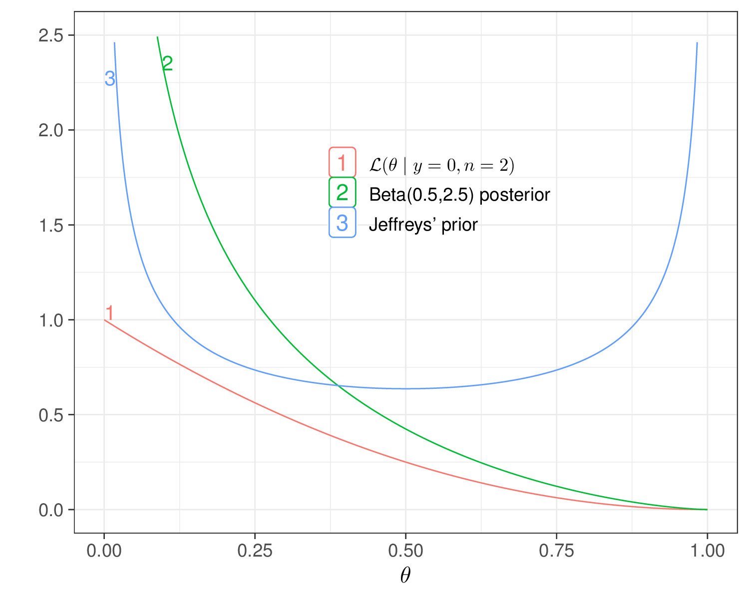
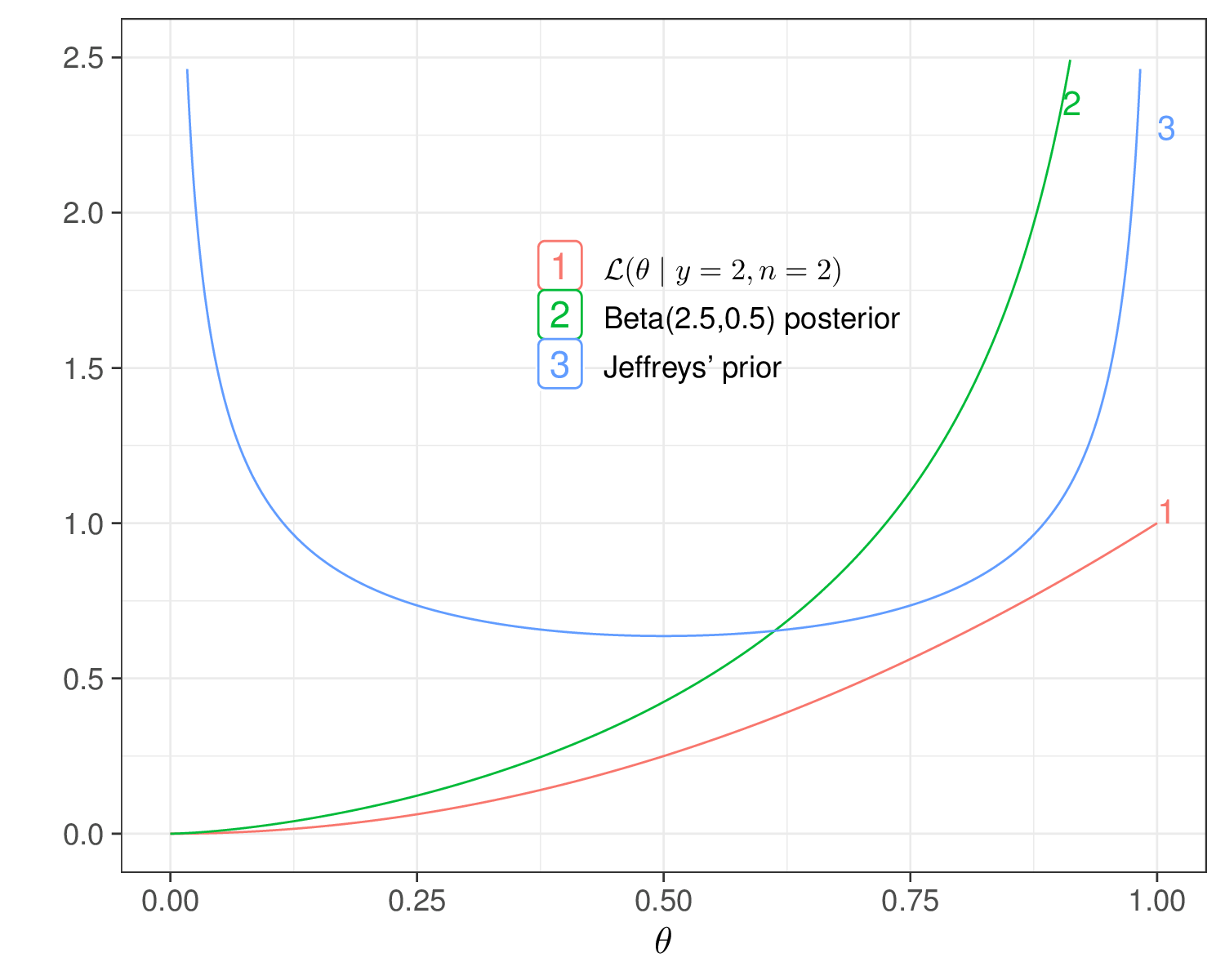
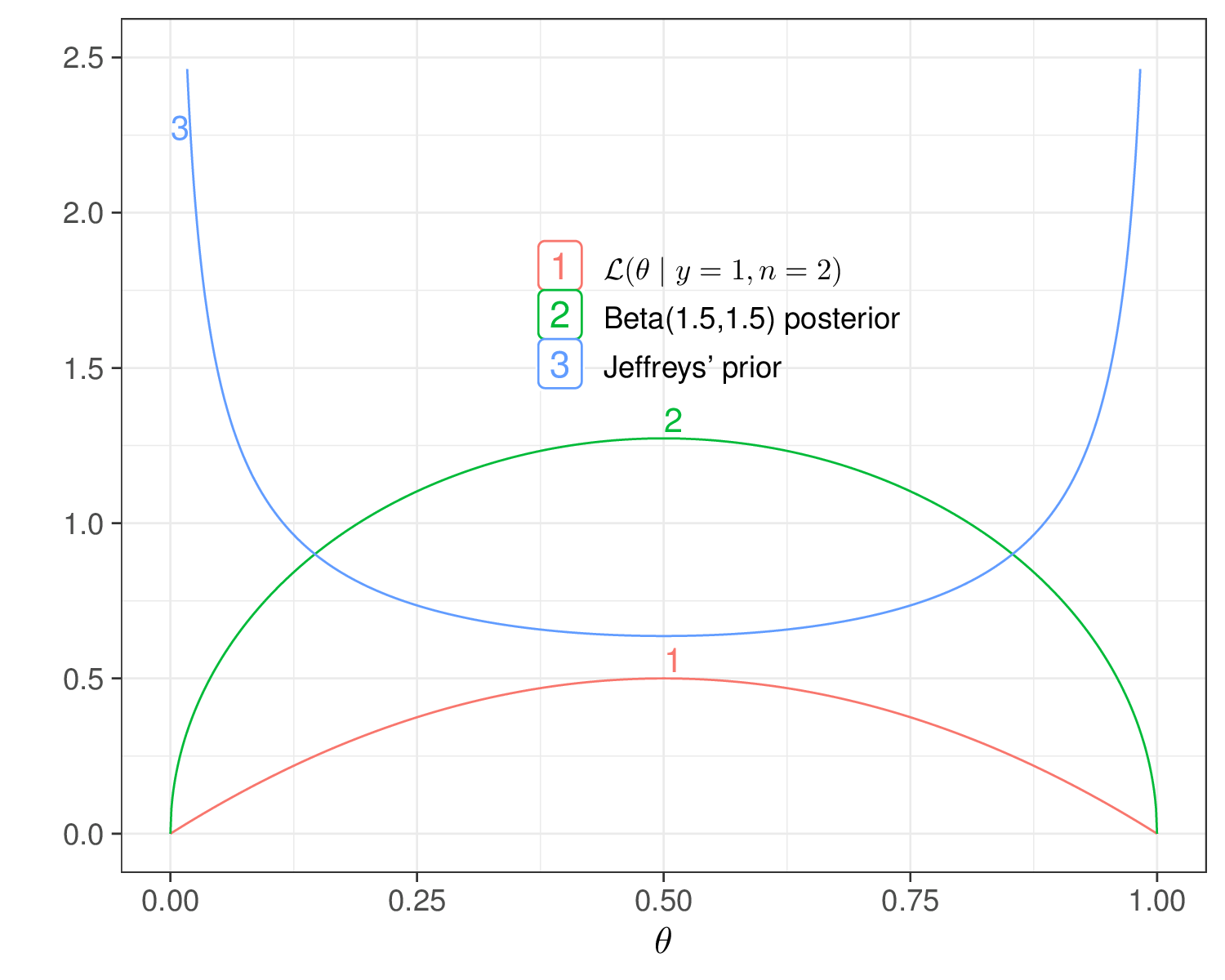
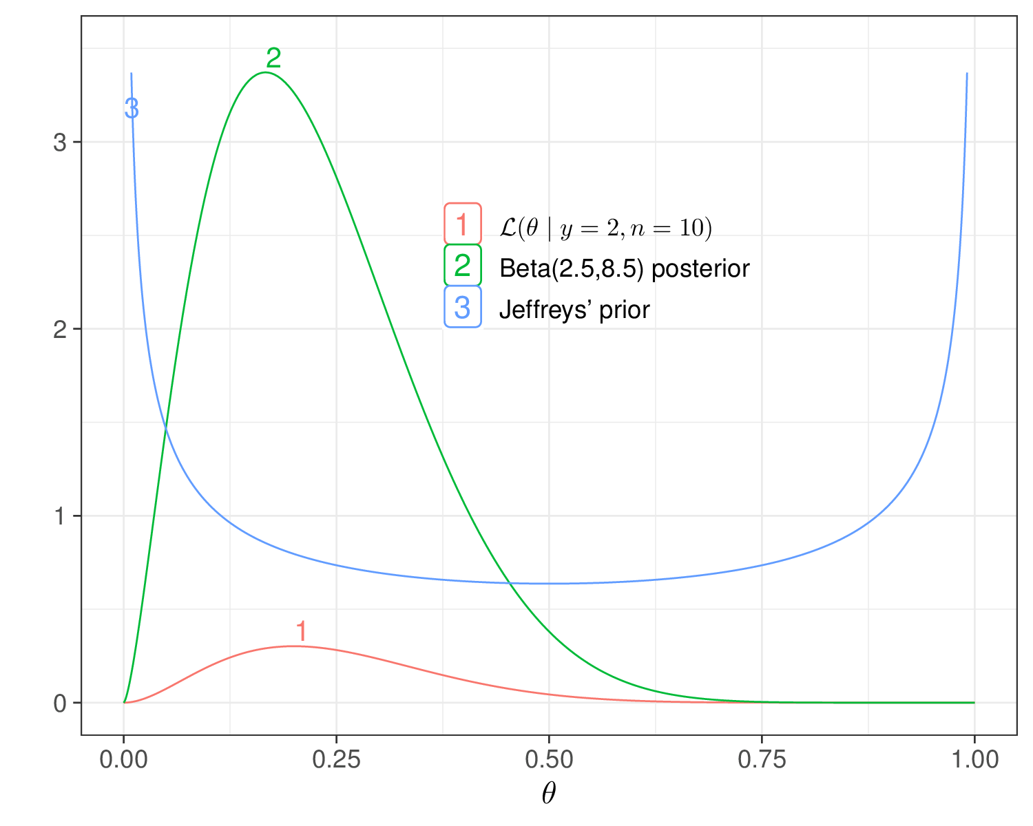
From the Bayesian statistical point of view, arguably they are a bit confusing and counter-intuitive, because, by definition, they completely discard any real and substantive information or belief we elicit in our prior. Back to the Binomial example, if we use Jeffreys’ prior, it is not true that we are willing to say that we strongly believe in its shape (i.e. that values at either extreme are very likely, but anything in between is extremely not plausible) – we just want to use that to limit the impact of the prior on the posterior.
Example 2.6. PC prior for Binomial parameter. Another simple example is for binary data recorded for a set of individuals, \(y_i \sim \text{Bernoulli}(\theta)\). We can consider as a “base-case” model the simple scenario in which \(\theta=0.5\) and thus set \(g=\text{Bernoulli}(\theta_0=0.5)\). We want to contrast this with the more flexible (and realistic) case in which \(\theta\) is unknown and can take on the values in \([0; 1]\), i.e. considering \(f=\text{Bernoulli}(\theta)\).
The KLD between two Bernoulli distributions with parameters \(\theta\) and \(\theta_0\), respectively, is \[ \begin{aligned} \text{KLD}(f,g) & =\sum_{y=0}^1 \theta^y(1-\theta)^{(1-y)}\log\left[ \left(\frac{\theta}{\theta_0}\right)^y \left(\frac{1-\theta}{1-\theta_0}\right)^{(1-y)} \right] \\ & = \log\left(\frac{\theta}{\theta_0}\right) \underbrace{\sum_{y=0}^1 y \theta^y(1-\theta)^{(1-y)}}_{\text{E}_{Y\mid\theta}[Y]} + \log\left(\frac{1-\theta}{1-\theta_0}\right) \underbrace{\sum_{y=0}^1 (1-y) \theta^y(1-\theta)^{(1-y)}}_{\text{E}_{Y\mid\theta}[1-Y]} \\ & = \theta \log\left(\frac{\theta}{\theta_0}\right) + (1-\theta)\log\left(\frac{1-\theta}{1-\theta_0}\right) \end{aligned} \] and thus \[d(\theta) = \sqrt{2\theta\log\left(\frac{\theta}{\theta_0}\right)+2(1-\theta)\log\left(\frac{1-\theta}{1-\theta_0}\right)}.\]
Using simple calculus properties, we can prove that for a generic function \(h(x)\), \(\displaystyle\frac{\partial h(x)^{1/2}}{\partial x} = \frac{h^{\prime}(x)}{2\sqrt{h(x)}}\). Applying this to \(d(\theta)\), we can then compute \[ \begin{aligned} \frac{\partial d(\theta)}{\partial \theta} & = \frac{\left[2\theta\log\left(\frac{\theta}{\theta_0}\right)+2(1-\theta)\log\left(\frac{1-\theta}{1-\theta_0}\right)\right]^\prime}{2d(\theta)} \\ & = \frac{1}{d(\theta)}\left[\log\left(\frac{\theta}{1-\theta}\right) - \log\left(\frac{\theta_0}{1-\theta_0}\right)\right] \end{aligned} \] and so we can derive the PC prior for \(\theta\) as \[p(\theta) = \lambda e^{-\lambda d(\theta)} \left\lvert \frac{1}{d(\theta)}\left[\log\left(\frac{\theta}{1-\theta}\right) - \log\left(\frac{\theta_0}{1-\theta_0}\right)\right] \right\rvert, \tag{2.10}\] for given baseline probability \(\theta_0\) and scaling factor \(\lambda\).
For example, we can set \(\lambda=1\) and use trial and error and numerical approximation (as in the R code below) to determine that this choice implies that about 22% of the probability mass exceed some arbitrary threshold of 0.75.
# Constructs a function with the definition of the PC prior
pc_prior=function(theta,theta0=0.5,lambda=1){
  # theta0 = baseline probability used in g(theta_0) - defaults at 0.5
  # lambda = scaling factor - defaults at 1

  # Computes the PC prior, guarding against singularity at d -> 0, in deriv
  d=sqrt(2*theta*log(theta/theta0) + 2*(1-theta)*log((1-theta)/(1-theta0)))
  deriv=ifelse(
    d<1e-10,1,abs((log(theta)-log(1-theta)-log(theta0)+log(1-theta0))/d)
  )
  lambda*exp(-lambda*d)*deriv
}

# Numerical integration of the function pc_prior()
# 1. selects a grid of values for theta
theta=seq(0,1,.0001)
# 2. uses the function integrate() to compute Pr(theta>0.5) under the density
# implied by the PC prior defined above. To do so, we select a grid of values
# from 0.5 to (almost) 1, as the integral must go from the value of u to 1...
u=seq(0.5,.9999,.01)
# 3. for each value in u, integrate the PC prior from that value of u up to 1
ints=list()
for (i in 1:length(u)) {
  ints[[i]]=integrate(pc_prior,u[i],1)
}
# 4. as we are only interested in the first element of the object 'cond'
# (named 'value'), we extract these and arrange them in a vector 'probs'
probs=numeric()
for (i in 1:length(ints)) {
  probs[i]=ints[[i]]$value
}
# NB: We could do more efficiently using 'lapply' and 'unlist'
ints=lapply(u,function(x) integrate(pc_prior,x,1))
probs=unlist(lapply(ints, `[[`,1))
# Normalises the probabilities (divide by the overall area under the density)
probs=probs/integrate(pc_prior,0,1)$value

# 5. searches the minimum value less than or equal to the set threshold alpha
alpha=0.22
u[min(which(probs<=alpha))]
[1] 0.75In other words, this prior encodes the assumption that we place around 80% chance on the fact that the underlying probability for the observed binary data is below 0.75, while keeping the impact of this prior to a minimum.
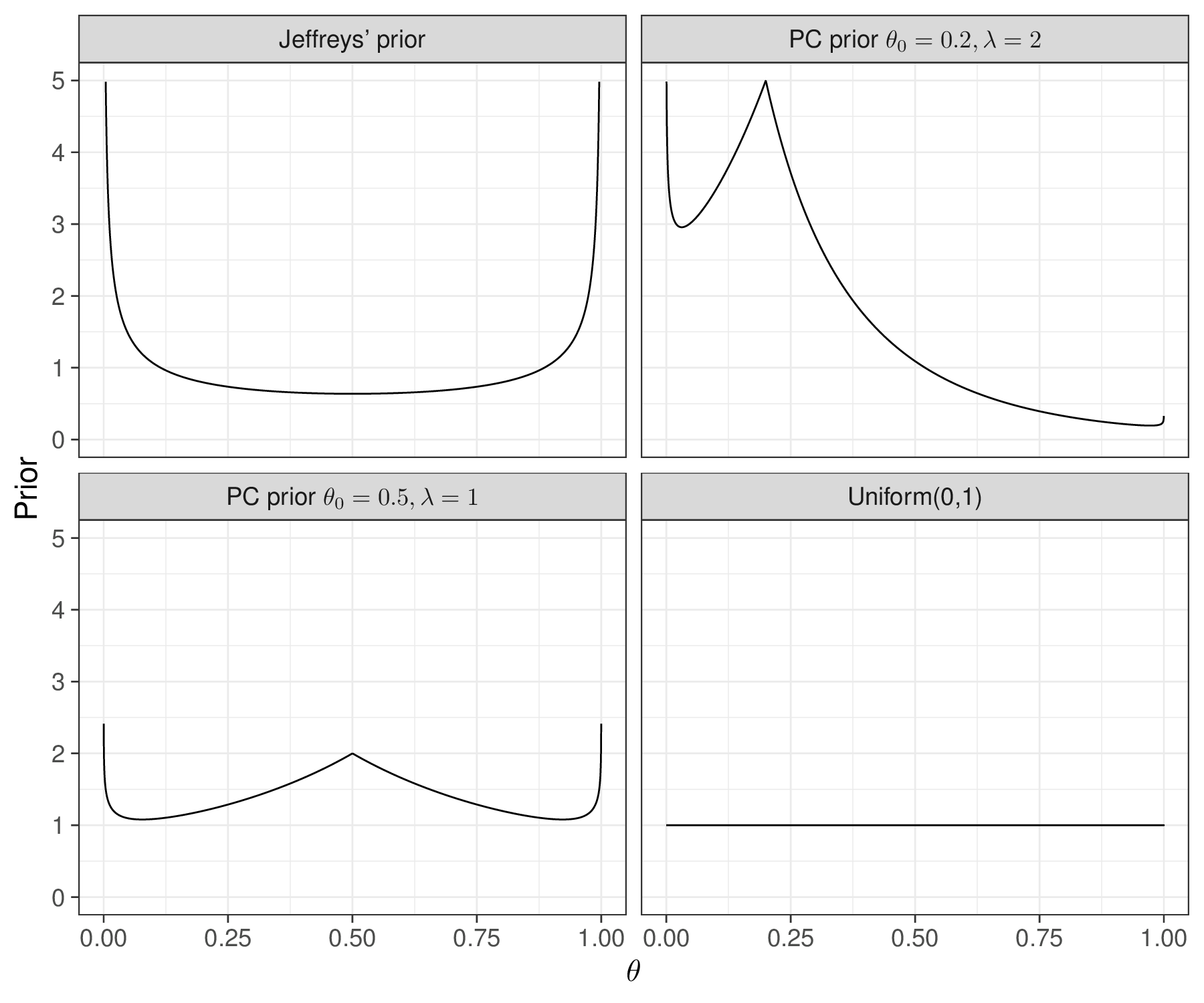
This can be appreciated by considering the very high probability associated with the tails of the resulting PC prior – cfr. this with the “standard” vague Uniform(0,1) and Jeffreys’ prior, a \(\text{Beta}(0.5,0.5)\), in Figure 2.10.
We also include in Figure 2.10 another PC prior, this time computed assuming a baseline probability \(\theta_0=0.2\) and a scaling factor \(\lambda=2\) – again, trial and error (and R code that can be adapted from the above), can show that this implies \(\Pr(\theta>0.75)\approx 0.04\).
Among other features (and unlike Jeffreys’ formulation), PC priors have the advantage of being invariant to reparameterisation even in multivariate cases and provide a principled way of including “minimal information” in the prior for the model parameters.
On the other hand, they may not be straightforward to think about and code up (we return to this point in Section 3.4), as well as requiring the specification of a “base case” prior model.
While representing a modern and principled version, as well as also overcoming some of the mathematical and practical limitations of “default” priors, PC priors have the disadvantage that they do not necessarily imply close-form computation of the posterior distribution. In all cases where it is not possible to either write down the posterior analytically, or to approximate it numerically (e.g. through MC simulation), Bayesian modelling has for the longest time remained more or less wishful thinking – until the perfect storm of cheap computing becoming increasingly available and very helpful algorithms borrowed from Physics have been discovered, in the mid-1990s.
2.3 Markov Chain Monte Carlo
Markov Chain Monte Carlo (MCMC) methods are a class of algorithms specifically designed to obtain samples from generic probability distributions (Gilks et al., 1996; Gamerman, 1997; Robert and Casella, 2004, 2010; Brooks et al., 2011; Gelman et al., 2013; Kruschke, 2015; McElreath, 2015).
To some extent, the first example of MCMC algorithm can be dated back to the 1950s, with what has then become famous as the “Metropolis algorithm” (Metropolis et al., 1953), later compounded by the work of Hastings (1970). The main idea underlying MCMC is that of a Markov chain, i.e. a sequence of random variables \(Y_0,Y_1,Y_2,\ldots\), for which the distribution of the future state of the process, given the current and the past values, does not depend on the whole history, but only on part of it. In the simplest case, only the immediate past \(t\) is relevant for the next state \(t+1\): \[ p(y_{t+1} \mid y_0,y_1,\ldots,y_t) = p(y_{t+1} \mid y_t) \tag{2.11}\] and the process is said to be of “order 1”, which we indicate in short as “Markov(1)”, but higher order dependence is possible.
To grossly simplify a rather complex methodology, MCMC methods are based on the construction of a Markov chain that converges to the desired target distribution \(p(\cdot)\) – this is the distribution from which we want to simulate; in a Bayesian context, this is the unknown posterior distribution of some parameter of interest.
Under rather broad regularity conditions, which are usually met by most practical problems (Gamerman, 1997; Jackman, 2009; Brooks et al., 2011; Kruschke, 2015; McElreath, 2015), after a sufficiently large number of iterations, the chain will forget the initial state and will converge to a unique stationary distribution, which does not depend on \(t\) or \(Y_0\). Once convergence is reached, it is possible to calculate any required statistic using Monte Carlo simulations.
NoteAnd the rest is history…
Robert and Casella (2011) present a brief history of MCMC in the context of statistical modelling. Interestingly, much of what is now considered landmark work in Statistics has a very firm grounding in other fields, notably Physics, where algorithms (e.g. the “Gibbs sampling” – see Section 2.3.1) were designed, typically to solve a very specific (and often limited) problem.
The seminal paper by Gelfand and Smith (1990) was able to link up the two literatures – recognising that what these algorithms could do was particularly helpful for the problem of Bayesian inference. Alan Gelfand tells the fascinating story of his encounter and subsequent collaboration with Adrian Smith in Carlin and Herring (2015).
2.3.1 Gibbs sampling
One of the most popular MCMC method is the Gibbs sampling (Geman and Geman, 1984; Gelfand and Smith, 1990), which can be considered as a specialised version of the Metropolis-Hastings algorithm.
If we assume that the model of interest is characterised by \(Q\) parameters, \(\boldsymbol\theta=(\theta_1,\theta_2,\ldots,\theta_Q)\), in the Bayesian context the objective is to obtain a representative sample from the marginal posterior distribution, given some relevant data \(\boldsymbol{y}\), for all the model parameters: \(p(\theta_1\mid \boldsymbol{y})\), \(p(\theta_2\mid \boldsymbol{y}),\ldots,p(\theta_Q\mid \boldsymbol{y})\), which we assume are not analytically available. Note that these are marginal distributions because, for any element of the parameter vector \(\theta_q\), they only depend on the observed data \(\boldsymbol{y}\) and not on the remaining parameters \(\boldsymbol\theta_{-q}=(\theta_1,\theta_2,\ldots,\theta_{q-1},\theta_{q+1},\ldots,\theta_Q)\).
The basic condition to run the Gibbs sampling is the ability to sample from the so-called “full-conditional” distributions \(p(\theta_1\mid\boldsymbol\theta_{-1},\boldsymbol{y}), p(\theta_2\mid\boldsymbol\theta_{-2},\boldsymbol{y}),\ldots,p(\theta_Q\mid\boldsymbol\theta_{-Q},\boldsymbol{y})\) – these are not the target of the Bayesian inference, because they condition on other parameters, as well as the observed data. Nevertheless, they may make life easier, in the end, because they condition on a larger number of variables, i.e. they have more variables to the right of the conditional sign “\(\mid\)”.
Schematically, the steps required to perform a MCMC simulation via Gibbs sampling are the following.
- Define an initial value to be arbitrarily assigned to the parameter of interest \(\theta^{(0)}_1,\theta^{(0)}_2,\ldots,\theta^{(0)}_Q\).
- Sample: \[\theta^{(1)}_1\sim p(\theta_1 \mid \theta^{(0)}_2,\theta^{(0)}_3,\ldots,\theta^{(0)}_Q,\boldsymbol{y})\] \[\theta^{(1)}_2\sim p(\theta_2 \mid \theta^{(1)}_1,\theta^{(0)}_3,\ldots,\theta^{(0)}_Q,\boldsymbol{y})\] \[\ldots\] \[\theta^{(1)}_Q\sim p(\theta_Q \mid \theta^{(1)}_1,\theta^{(1)}_2,\ldots,\theta^{(1)}_{Q-1},\boldsymbol{y}).\]
- Repeat step 2. for \(S\) times until convergence is reached (see Section 2.3.2) and produce a sample from the distribution \(p(\boldsymbol\theta \mid y)\) using Monte Carlo simulations.
We can think of this as a sampling process where we “fix” the value of all the other parameters \(\boldsymbol\theta_{-q}\) and only sample the remaining one \(\theta_q\). The intuition as to why this actually work is that if we were able to do this repeated sampling for \(\infty\) times, we would have a grid for \(\boldsymbol\theta_{-q}\) with so many values that, effectively, we will have accounted for all the possible configurations in the marginal distribution \(p(\theta_q\mid\boldsymbol{y})\).
Effectively, this process marginalises out the uncertainty in the other parameters \[p(\theta_q\mid\boldsymbol{y})=\int p(\theta_q\mid\boldsymbol{y},\boldsymbol\theta_{-q})p(\boldsymbol\theta_{-q})d\boldsymbol\theta_{-p}.\]
Another way to see this is to think that, more or less, \[p(\theta_q\mid\boldsymbol\theta_{-q},\boldsymbol{y}) \approx p(\theta_q\mid\boldsymbol{y})\] and if we have very many values of \(\boldsymbol\theta_{-q}\), this approximation is pretty good.
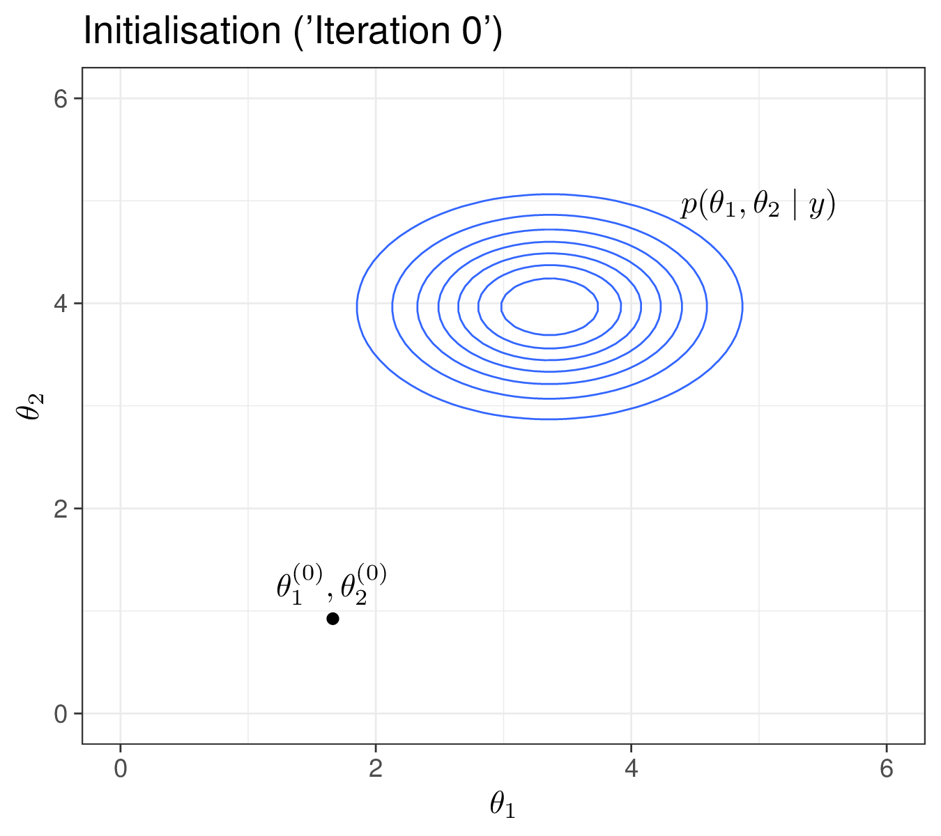
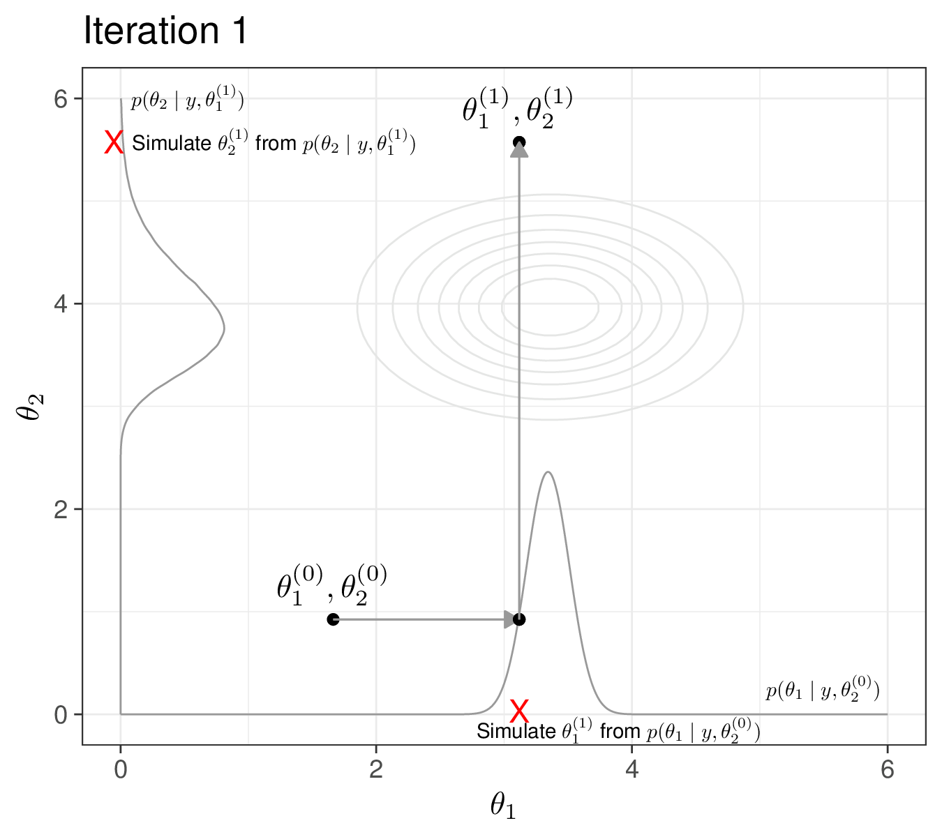
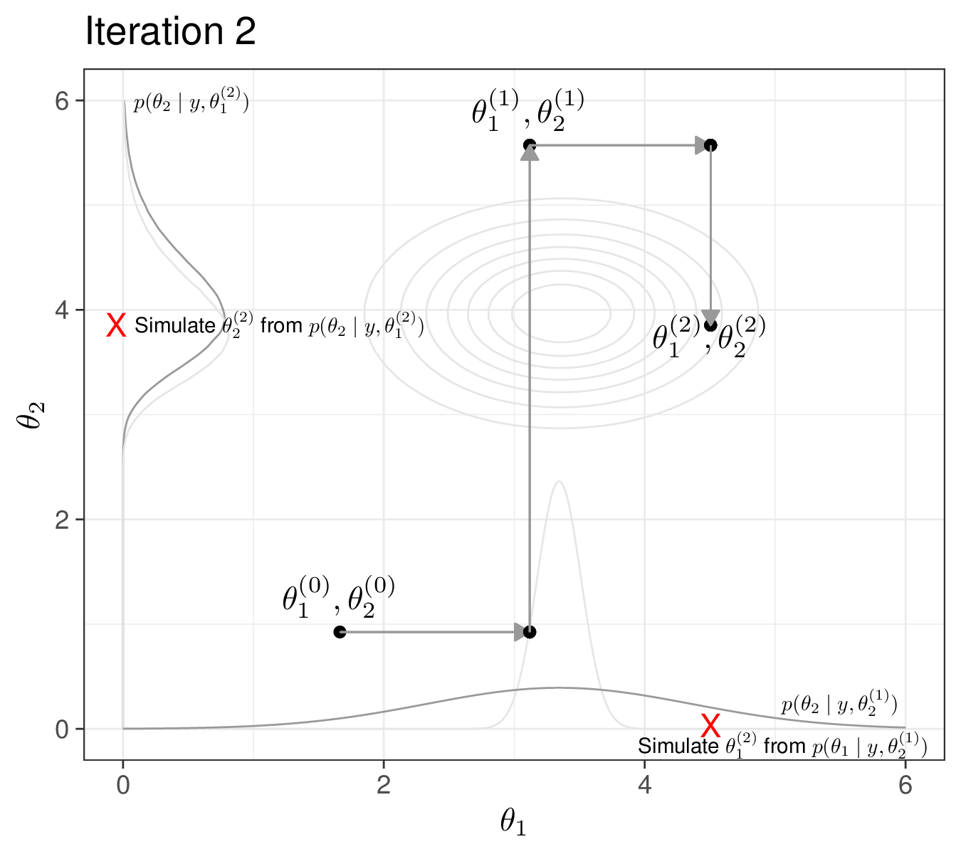
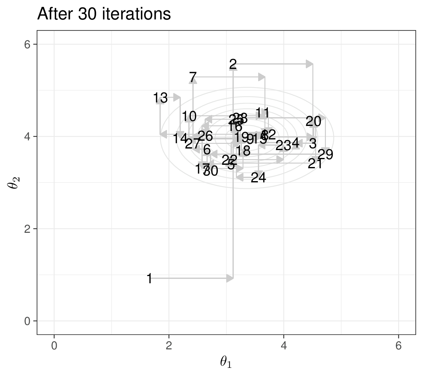
Figure 2.11 shows a graphical visualisation of this process, considering a vector of \(Q=2\) parameters \(\boldsymbol\theta=(\theta_1,\theta_2)\). In Figure 2.11 (a), we show the “true”, underlying target distribution, indicated as \(p(\theta_1,\theta_2\mid y)\) – of course, in practice we do not know this (and that is the reason why we are running the MCMC algorithm in the first place!). We also highlight the initial point \((\theta_1^{(0)},\theta_2^{(0)})\). As is possible to see, we have (perhaps randomly) chosen a value that is actually quite far from the target distribution.
In Figure 2.11 (b), we consider the first iteration of the process. First, we fix \(\theta_2\) to its current value (the initialisation \(\theta_2^{(0)}\)) and we simulate from the full conditional \(p(\theta_1\mid y,\theta_2^{(0)})\), depicted as the curve on the \(x\)–axis. The simulated value is the point indicated by the cross along the \(x\)–axis and we can label it as \(\theta_1^{(1)}\). This is the first move from the initialisation point – the arrow going from \((\theta_1^{(0)},\theta_2^{(0)})\) moving along the \(x\)–axis. Then, we fix \(\theta_1\) to the new current value \(\theta_1^{(1)}\) and simulate a new value for \(\theta_2\) from the full conditional \(p(\theta_2\mid y,\theta_1^{(1)})\), depicted as the curve along the \(y\)–axis. The simulated point \(\theta_2^{(1)}\) is again indicated with the cross on the \(y\)-axis. With this, we have now completed the first iteration and a full move from \((\theta_1^{(0)},\theta_2^{(0)})\) to \((\theta_1^{(1)},\theta_2^{(1)})\).
Figure 2.11 (c) shows the second iteration. We simulate from the current full conditional \(p(\theta_1\mid y,\theta_2^{(1)})\), which again is the curve along the \(x\)–axis. Notice that we have greyed out the previous full conditional (which we used at iteration 1); the current distribution has a much wider variance, which is consistent with the fact that the previous one was conditional on a smaller value for \(\theta_2\) (this would be obvious, if for instance \(\theta_1\) was a location parameter, e.g. a mean and \(\theta_2\) was a scale parameter, e.g. a variance – cfr Example 2.7). The new simulated value for \(\theta_1\), indicated as \(\theta_1^{(2)}\) is again the cross along the \(x\)–axis. Then, we compute the new full posterior \(p(\theta_2\mid y,\theta_1^{(2)})\) and use it to draw a random value \(\theta_2^{(2)}\), the red cross along the \(y\)–axis. Again, we grey out the previous full conditional along the \(y\)–axis – that is not relevant anymore, because we are conditioning on a different value for \(\theta_1\).
Finally, Figure 2.11 (d) shows the MCMC trajectory for the first 30 iterations. Starting from the point labelled as 1 (the initialisation) all the way to the point labelled as 30. As we can see, while some simulations are outside of the target area, many do cover the part of the parametric space for \(\boldsymbol\theta\). Depending on the problem, the choice of the initial values may be crucial in getting us to visit consistently the relevant portion of the parametric space – and, crucially, the first batch of iteration may be highly biased, i.e. visit parts of the parametric space that have negligible probability mass under the target (posterior) distribution. We return to these two points in Section 2.3.2.
Example 2.7. Semi-conjugated model. Consider the following model: \[\begin{eqnarray*} \boldsymbol{y}=(y_1,y_2,\ldots,y_n) & \stackrel{iid}{\sim} & \text{Normal}(\mu,\sigma^2),\\ \mu & \sim & \text{Normal}(\mu_0,\sigma^2_0) \\ \tau = \frac{1}{\sigma^2} & \sim & \text{Gamma}(\alpha_0,\beta_0) \end{eqnarray*}\]
Under these assumptions we can prove analytically (Gelman et al., 2013) that the full conditional distributions for the two parameters \(\mu\) and \(\tau\) are \[\mu\mid \sigma^2,\boldsymbol{y} \sim \text{Normal}(\mu_1,\sigma^2_1) \qquad \mbox{with: } \mu_1=\sigma^2_1\left( \frac{\mu_0}{\sigma^2_0} + \frac{n\bar{y}}{\sigma^2}\right) \qquad \mbox{and: } \quad \sigma^2_1=\left(\frac{1}{\sigma^2_0}+\frac{n}{\sigma^2}\right)^{-1}\] (cfr. Equation 2.8) and \[\tau\mid\mu,\boldsymbol{y} \sim \text{Gamma}(\alpha_1,\beta_1) \qquad \mbox{with: }\,\alpha_1=\alpha_0+\frac{n}{2}\quad \mbox{and: } \quad \beta_1 = \beta_0 + \frac{1}{2}\sum_{i=1}^n (y_i-\mu)^2\] (cfr. Equation 2.9).
Notice that this example does not really require Gibbs sampling or any form of MCMC to estimate the joint posterior distribution for the parameters and, in fact, we could determine the form of the posterior distributions for both \(\mu\mid \boldsymbol{y}\) and \(\sigma \mid \boldsymbol{y}\). However, because of its specific assumptions it is very helpful because essentially we can determine analytically the full conditional distributions for each parameter (details later). This means that we can directly and repeatedly sample from them (which is a pre-requisite of Gibbs sampling and what software such as BUGS do – see Chapter 3).
Notice that the full conditionals are not the target distributions for Bayesian inference. What we really want is the marginal posterior distributions \(p(\mu \mid \boldsymbol{y} )\) and \(p(\tau \mid \boldsymbol{y})\), which can be simply obtained from the joint posterior \(p(\mu, \tau \mid \boldsymbol{y})\).
NoteMarginalisation
The main intuition here is to do with the basic properties of conditional probabilities. Recall that given two events \(A\) and \(B\), then by definition \(\Pr(A \mid B) = \displaystyle\frac{\Pr(A,B)}{\Pr(B)}\).
Now we can extend this to the case of three events \(A\), \(B\) and \(C\), by adding \(C\) to the conditioning set (i.e. to the right of the “\(\mid\)” symbol throughout the equation) and get \(\Pr(A \mid B, C ) = \displaystyle\frac{\Pr(A,B\mid C)}{Pr(B\mid C)}\). If we replace \(\mu\) for \(A\), \(\sigma^2\) for \(B\), \(\boldsymbol{y}\) for \(C\) and a probability distribution \(p(\cdot)\) for the probability associated with an event \(\Pr(\cdot)\), we can write \[p(\mu \mid \sigma^2, \boldsymbol{y} ) = \frac{p(\mu,\sigma^2\mid \boldsymbol{y})}{p(\sigma^2\mid \boldsymbol{y})}\propto p(\mu, \sigma^2 \mid \boldsymbol{y}).\]
Similarly, \[p(\sigma^2 \mid \mu, \boldsymbol{y}) = \frac{p(\mu,\sigma^2\mid\boldsymbol{y})}{p(\mu\mid\boldsymbol{y})} \propto p(\mu,\sigma^2\mid\boldsymbol{y}).\] We can then see that each full conditional is proportional to the target distribution (i.e. the joint posterior of all the parameters).
Thus, sampling repeatedly from all the full conditionals essentially gives us something that is, broadly speaking, proportional to our target joint posterior distribution. Formal theorems ensure that if we do this long enough, we are guaranteed to actually approximate the target to an arbitrary degree of precision – see also Figure 2.12.
In this case, for each of the two parameters, conditionally on (i.e. given) the other, the posterior is in the same family of the prior – the posterior for \(\mu\mid\boldsymbol{y},\sigma^2\) is still a Normal and the posterior for \(\tau\mid\boldsymbol{y},\mu\) is still a Gamma; what changes is the value of the “hyper-parameters” (i.e. the parameters of these distributions), which move from (\(\mu_0\), \(\sigma_0^2)\) to \((\mu_1 , \sigma_1^2 )\) and from \((\alpha_0, \beta_0 )\) to \((\alpha_1 , \beta_1)\). For this reason, this model is called “semi-conjugated”.
These relationships clarify that the (posterior) distribution of the mean \(\mu\) depends (among other things) on the variance \(\sigma^2 = 1/\tau\) as well as that the posterior for the precision \(\tau\) depends (among other things) on the mean \(\mu\). Crucially, in this example, this dependence is known in closed form. A very useful implication of this set up is that it means that we can directly determine not just the distributional form of the full conditionals (Normal for the mean and Gamma for the precision), but also the numerical value of the “hyper-parameters” (\(\mu_1, \sigma_1^2 , \alpha_1,\beta_1 )\).
NoteWhat do we really need to do?
We need to create a routine that can simulate sequentially from these distributions, with the aim of obtaining a sample from the joint posterior distribution \(p(\mu, \tau \mid \boldsymbol{y})\). So, once the data \(\boldsymbol{y}\) have been observed and we have fixed the values for the parameters of the prior distributions (\(\mu_0, \sigma_0^2,\alpha_0,\beta_0)\), we can use for instance R, to simulate from the resulting full conditionals.
At each iteration, we will update sequentially the values of the two parameters: first we update \(\mu\) by simulating from its full conditional, then we set the value of \(\mu\) to the one we have just simulated and update the value of \(\tau\) by randomly drawing from its full conditional. And we repeat this process “until convergence”.
Data and fixed quantities
Suppose we have observed a sample of \(n = 30\) data points, for example, in R you may input the data onto your workspace using the following command.
# Vector of observed data
y = c(
  1.2697,7.7637,2.2532,3.4557,4.1776,6.4320,-3.6623,7.7567,5.9032,
  7.2671,-2.3447,8.0160,3.5013,2.8495,0.6467,3.2371,5.8573,-3.3749,
  4.1507,4.3092,11.7327,2.6174,9.4942,-2.7639,-1.5859,3.6986,2.4544,
  -0.3294,0.2329,5.2846
)
Assume also that you want to set the value of the parameters for the priors as \(\mu_0 = 0\), \(\sigma_0^2 = 10000\) and \(\alpha_0 = \beta_0 = 0.1\). In R we could define these using the following commands.
# "Hyper-parameters" (ie parameters for the prior distributions)
mu_0 = 0
sigma2_0 = 10000
alpha_0 = 0.01
beta_0 = 0.01
These are of course arbitrary values and we may have more specific knowledge to set them to different numbers.
We may also want to define some “utility” variables, that can be used later on, for instance the sample size and observed sample mean, which we can input in R as in the following code.
# Sample size and sample mean of the data
n = length(y)
ybar = mean(y)
The actual values of these variables are now stored in the respective R “objects” and can be accessed at any point. For instance, we can simply call the name of the objects to output the sample size and mean.
n[1] 30ybar[1] 3.343347Initial values
In order to run the Gibbs sampling algorithm, we need to initialise the Markov chains. This essentially means telling the computer what values should be used at iteration 0 of the process for anything that is a) associated with a probability distribution (i.e. it is not known with absolute certainty); and b) has not been observed.
In this case, the variables that are modelled with a probability distribution but are not observed are \(\mu\) and \(\tau\); \(\boldsymbol{y}\) is also associated with a probability distribution, but as it is observed, the MCMC algorithm does not require any further input.
We can do this in R using the following code.
# Sets the "seed" (for reproducibility). With this command, you will
# *always* get the exact same output
set.seed(13)
# Initialises the parameters
mu = tau = numeric()
sigma2 = 1/tau
mu[1] = rnorm(1,0,3)
tau[1] = runif(1,0,3)
sigma2[1] = 1/tau[1]
First, we set the “random seed” (in this case to the totally arbitrary value 13), which ensures replicability of the results. If we run this code on any machine, we will always and invariably obtain the same results.
Then, we define the parameters mu and tau to be vectors, which in R we do by using the R built-in command function numeric(). Basically, the command mu = tau = numeric() instructs R to expect these two objects to be vectors of (as yet) unspecified length (if we used the command x = numeric(5), we would define a vector of length 5).
Finally, we set the first value of mu and tau to be randomly generated, respectively from a Normal(mean = 0, sd = 3) and a Uniform(0, 3). Again, this is arbitrary and we may decide instead to specify a fixed, set initial point, e.g. mu[1]=2 and tau[1]=5 – this would also work, provided the given values are consistent with the probabilistic assumptions made for the underlying variable (thus, for instance, tau[1]=-5 would simply break the process).
We can check the values that have been selected to initialise your Markov chain by simply typing the name of the variables (or some suitable function thereof).
mu[1] 1.662981sqrt(sigma2)[1] 0.9249339Running the Gibbs sampling
Generally speaking, the actual Gibbs sampling is really simple (if the full conditionals are known analytically!) and reduces to code such as the following.
# Sets the number of iterations (nsim)
nsim = 1000
# Loops over to sequentially update the parameters
for (i in 2:nsim) {
  # 1. Updates the sd of the full conditional for mu
  sigma_1 = sqrt(1/(1/sigma2_0 + n/sigma2[i-1]))
  # 2. Updates the mean of the full conditional for mu
  mu_1 = (mu_0/sigma2_0 + n*ybar/sigma2[i-1])*sigma_1^2
  # 3. Samples from the updated full conditional for mu
  mu[i] = rnorm(1,mu_1,sigma_1)
  # 4. Updates the 1st parameter of the full conditional for tau
  alpha_1 = alpha_0+n/2
  # 5. Updates the 2nd parameter of the full conditional for tau
  beta_1 = beta_0 + sum((y-mu[i])^2)/2
  # 6. Samples from the updated full conditional for tau
  tau[i] = rgamma(1,alpha_1,beta_1)
  # 7. Re-scales the sampled value on the variance scale
  sigma2[i] = 1/tau[i]
}
The code above matches perfectly the mathematical expressions defined for the (updated) parameters of the full posterior distributions. The loop goes from 2 to nsim – the first value of the vectors mu, tau and sigma2 are filled at initialisation. Note that there is a slight inconsistency in the terminology: usually, we refer the initialisation of the process as “iteration 0” (see for instance in Figure 2.11. However, R does not let us index a vector with the number 0, i.e. the first element of a vector is indexed by the number 1. Thus, what we would in general indicate as \(\mu^{(0)}\) to highlight the pre-algorithm stage, is actually written as mu[1] in the R code. Similarly, the updated value for \(\mu\) at iteration 2 is indicated as \(\mu^{(2)}\) if we start from \(\mu^{(0)}\), but as mu[3] in the R code.
Note that the code above produces simulations from the full conditional of the precision \(\tau\) , which are then rescaled to produce a vector of simulations from the joint posterior distribution for the variance \(\sigma^2\) . It is of course very easy to also rescale these further to obtain a sample of values from the posterior of the standard deviation \(\sigma\), for example using the code sigma=sqrt(sigma2). This is a point we have already made in Section 1.2.3.
Once this code has been executed in R our output is made by vectors that, if the procedure has worked (i.e. it has converged), are drawn, at least with a very good degree of approximation, from the joint posterior distribution of the parameters.
2.3.2 Diagnostics: checking convergence and autocorrelation
For any MCMC algorithm, we need to make sure that the results we use for the Monte Carlo analysis are indeed representative of the underlying target posterior distribution. Figure 2.11 shows that the starting point may in general be very distant from the target area – of course, we do not know where the true posterior probability is in the parametric space (that is the reason why we run the MCMC procedure in the first place), but we need to account for the possibility that it may take us some time to consistently reach and sample from the core of the target posterior distribution.
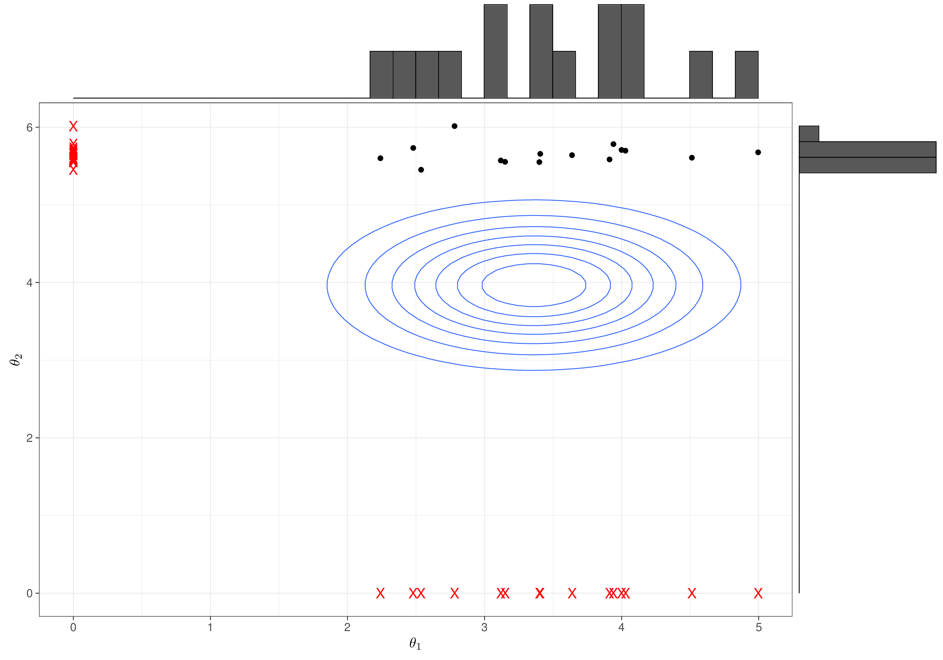
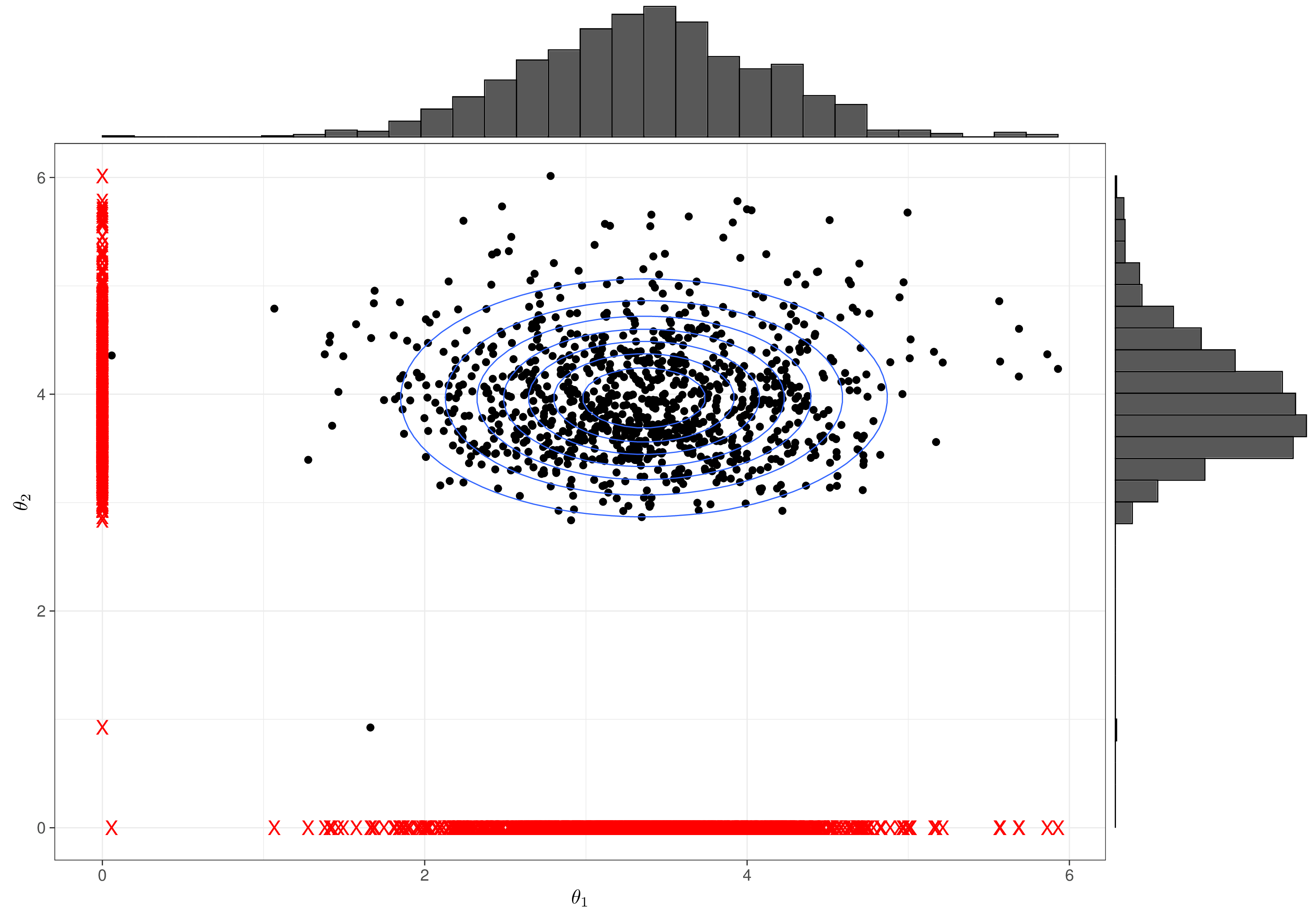
Intuitively, if we only have a small number of iterations (say, 15, as in Figure 2.12 (a)), we are not really exploring the range of the two marginal distributions (for \(\theta_1\) along the \(x\)–axis and for \(\theta_2\) along the \(y\)–axis). Thus, the simulations from the full conditionals (red crosses along the axes) are not a good representation of the posteriors.
However, if we run the process for long enough (in theory, for \(\infty\) times; Figure 2.12 (b) uses 1000 iterations), then we do cover the full range of the parameters and so the samples that we obtain can be used to describe the two posterior distributions (e.g. the histograms on the top and right sides of the plots).
There are perhaps two main implications:
- The first few simulated values, starting from the initialisation, could be very different from representative samples from the target posterior distribution;
- We need to select a large enough number of simulations to be reasonably sure that we are, in fact, covering the true target posterior distribution.
Burn-in and convergence
Probably the most obvious way to remedy the first issue is to run the MCMC process for long enough, so that we can simply discard the “first few” iterations, as they are potentially non-representative of the target posterior distribution. This batch of iterations to be discarded is often termed the “burn-in” (or the “warm-up”). Interestingly, this aspect was not immediately understood when the Gibbs sampling algorithm became popular in Statistics, in the mid-1990s.
Of course, as we do not know what the target distribution is, it is also difficult to assess how long should the burn-in be; for this reason, when the problem became clear (and computation became increasingly cheaper), researchers started to suggest running two or more parallel Markov chains, starting from different initial values.
Figure 2.13 shows this graphically. Here, we start Chain 1 (the darker curve) from a very large value for the parameter of interest (close to 200) and Chain 2 (the lighter one) from a value at the opposite end of the spectrum in the likely range of the parameter. For the first 250 iterations or so, the two traceplots go their separate way, trying to find the target posterior distribution. At about iteration 250, they start to consistently be on top of each other, indicating that they are now visiting the same portion of the parametric space. Eye-balling the traceplot is a relatively easy way of checking convergence, i.e. that irrespective of where we started from, we have now reached the relevant target distribution and are consistently simulating from it.
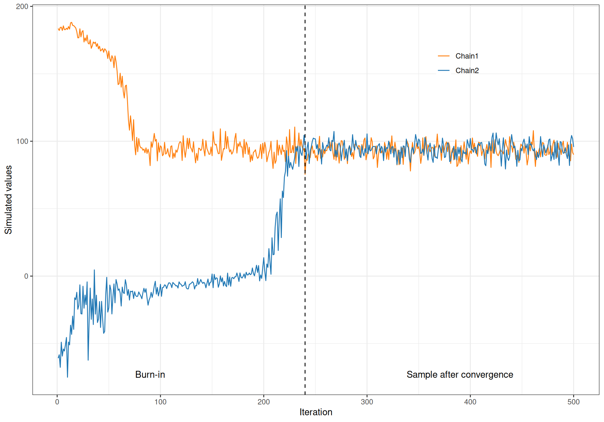
This process can drive our choice in the burn-in period. If, for instance, in the example of Figure 2.13, we had decided to initially run the MCMC algorithm for 200 iterations, using the two separate chains would allow us to clearly see an obvious lack of convergence, indicating the need to run it for longer.
We can also run more formal diagnostics to check if multiple chains end up in essentially same place. Perhaps one of the most popular is the Brooks-Gelman-Rubin statistic, more often referred to as Potential Scale Reduction (PSR), or \(\hat{R}\) (Brooks and Gelman, 1998; Gelman and Rubin, 1992). This is based on ratio of between- to within-variances of multiple chains, formally defined as \[{\hat{R}}=\sqrt{{\frac{1}{W}}{\left(\frac{n_{\text{\textit{sims}}}-1}{n_{\text{\textit{sims}}}}W + \frac{1}{n_{\text{\textit{chains}}}}B\right)}} \tag{2.12}\] where: \[W =\text{E}\left[\hat{\sigma}^2_1,\ldots,\hat{\sigma}^2_{n_{\text{\textit{chains}}}}\right] \quad \mbox{and}\quad B =\displaystyle n_{\text{\textit{sims}}}\text{Var}\left[\hat{\mu}_1,\ldots,\hat{\mu}_{n_{\text{\textit{chains}}}}\right]\] with \((\hat\mu_c,\hat{\sigma}_c^2)\) indicating the sample mean and variance for the \(n_{\text{\textit{sims}}}\) simulations in the \(c\)-th of the \(n_{\text{\textit{chains}}}\) used.
Heuristically, the ratio of \(\displaystyle\left(\frac{n_{\text{\textit{sims}}}-1}{n_{\text{\textit{sims}}}}W + \frac{1}{n_{\text{\textit{sims}}}}B\right)\) to \(W\) should converge to 1 as iterations increase, because, intuitively, this would indicate a situation where the variance within chains is approximately the same as the variance between chains. This in turn would suggest that the chains are subject to some healthy variation and they are both visiting the same portion of the parametric space.
For the example shown in Figure 2.13, we can compute the PSR using the following code.
# Here 'x' is a matrix containing 500 rows (simulations) and 2 columns (chains)
# We can show the first 4 rows of this matrix using the command
x |> head(4)
Chain 1 Chain 2
[1,] 183.6060 -60.85966
[2,] 182.1367 -58.33558
[3,] 184.3697 -67.64598
[4,] 184.5805 -49.01882# Now create a little function to compute the value of PSR
Rhat=function(x) {
# Number of simulations (rows of x)
nsims=nrow(x)
# Number of chains (columns of x)
nchains=ncol(x)
# Vector of variances for the simulated values in each chain
sigma2.hat=apply(x,2,var)
# Vector of means for the simulated values in each chain
mu.hat=apply(x,2,mean)
# Computes W and B
W=mean(sigma2.hat)
B=nsims*var(mu.hat)
# Now computes and returns the PSR
((((nsims-1)/nsims)*W+B/nsims)/W) |> sqrt()
}
# Now compute PSR for the whole 500 simulations
Rhat(x)[1] 1.368965# And compute PSR from simulation 250
Rhat(x[250:500,])[1] 1.002365We first create a little function that uses the simulated values (stored in the object x, of which we show the first few rows) to obtain the approximated value for PSR, exactly matching Equation 2.12. As is possible to see, when we use the whole set of 500 simulations for the two chains, the value of \(\hat{R}=1.368965>>1\), indicating lack of convergence. When we restrict the sample to the simulations after the 250-th iteration (as inspected in the traceplot of Figure 2.13), we get \(\hat{R}=1.002365\), which is now, consistently with the traceplot, closer to 1 and thus indicates convergence.
Autocorrelation
Because of how MCMC algorithms – and especially the Gibbs sampling – work, another issue to consider carefully when assessing the validity of a set of simulations to be used for MC estimation of a quantity of interest is the information load that it carries. The main reason for this is that, because of how they are obtained, successive MCMC iterations tend to be correlated. The \(s\)-th simulation for the \(q\)-th element of the parameter vector \(\boldsymbol\theta=(\theta_1,\ldots,\theta_Q)\) is obtained from the full conditional distribution where \(\boldsymbol\theta_{-q}\) are fixed to the value simulated last.
NoteInformation vs correlation
Here the main idea is that a sample of \(S\) simulated values may not actually contribute the same amount of information that the nominal sample size suggest. If we had \(S\) independent data points, then each would contribute 1 “information point” and thus the overall sample information load would be, intuitively, \(S\). But because of correlation, it is likely that the information load is overall less than \(S\).
Consider for instance a survey in which you want to collect information on the frequency of surnames. You may go around households and ask for the surname of the people living in a given one. Imagine that the first house you hit is a shared accommodation, where University students live. Because they are totally unrelated (i.e. statistically independent, as far as their surname is concerned), if you observe 4 data points (= people), you will probably get 4 separate responses, which means an overall “information load” of 4.
Imagine now that your next household is a traditional family home, where the 4 residents all share the same surname. In this case, while the number of data points is the same as before, the information load is simply 1 – because of the fact that all the residents are correlated, then every response contribute only 1 “information point”, combined.
The consequence of the above issue is that if the MCMC sample is highly autocorrelated (i.e. successive iterations, even at higher lags, for instance every other \(l\)), then \(S\) data points will contribute a much lower “effective sample size” (ESS, see Lunn et al., 2013; Raftery and Lewis, 1992). This can be formally defined as \[ n_{\text{\textit{eff}}}=\frac{n_{\text{\textit{sims}}}}{1+2\sum_{l=1}^\infty \rho_l}, \tag{2.13}\] where \(\displaystyle\rho_l = \frac{\text{Cov}\left(\theta^{(t)},\theta^{(t+l)}\right)}{\text{Var}\left(\theta\right)}\) is the autocorrelation between two simulations separated by a lag \(l\).
We can provide an approximation to the ESS by computing \[n_{\text{\textit{eff}}}\approx n_{\text{\textit{chains}}}n_{\text{\textit{sims}}}\min\left[ \frac{1}{B}\left( \frac{n_{\text{\textit{sims}}}-1}{n_{\text{\textit{sims}}}}W + \frac{B}{n_{\text{\textit{sims}}}}\right), 1 \right], \tag{2.14}\] which is a measure of the equivalent number of independent observations to the correlated MCMC sample.
We can use Equation 2.14 and compute the ESS for both the whole sample in the object x (made by 500 iterations per chain) and the one restricted to the last 250 iterations and get values of \(n_{\text{\textit{eff}}}=4.28\) and \(n_{\text{\textit{eff}}}=230.47\), respectively. The sample “at convergence” has a much larger ESS, which is closer to the nominal sample size (250 iterations per chain, so 500 in total), although still lower, by effect of the intrinsic autocorrelation.
In addition to this analysis, we can use the following R code and the bmhe function acfplot() to visualise the amount of temporal correlation in the simulated values in Figure 2.14.
# Stacks the two chains into a vector of 500x2 iterations & plots AC function
c(x) |> bmhe::acfplot() +
  labs(title="Autocorrelation for all 1000 iterations")
# Stacks the two chains into a vector of 250x2 iterations & plots AC function
c(x[250:500,]) |> bmhe::acfplot() +
  labs(title="Autocorrelation for the last 500 iterations")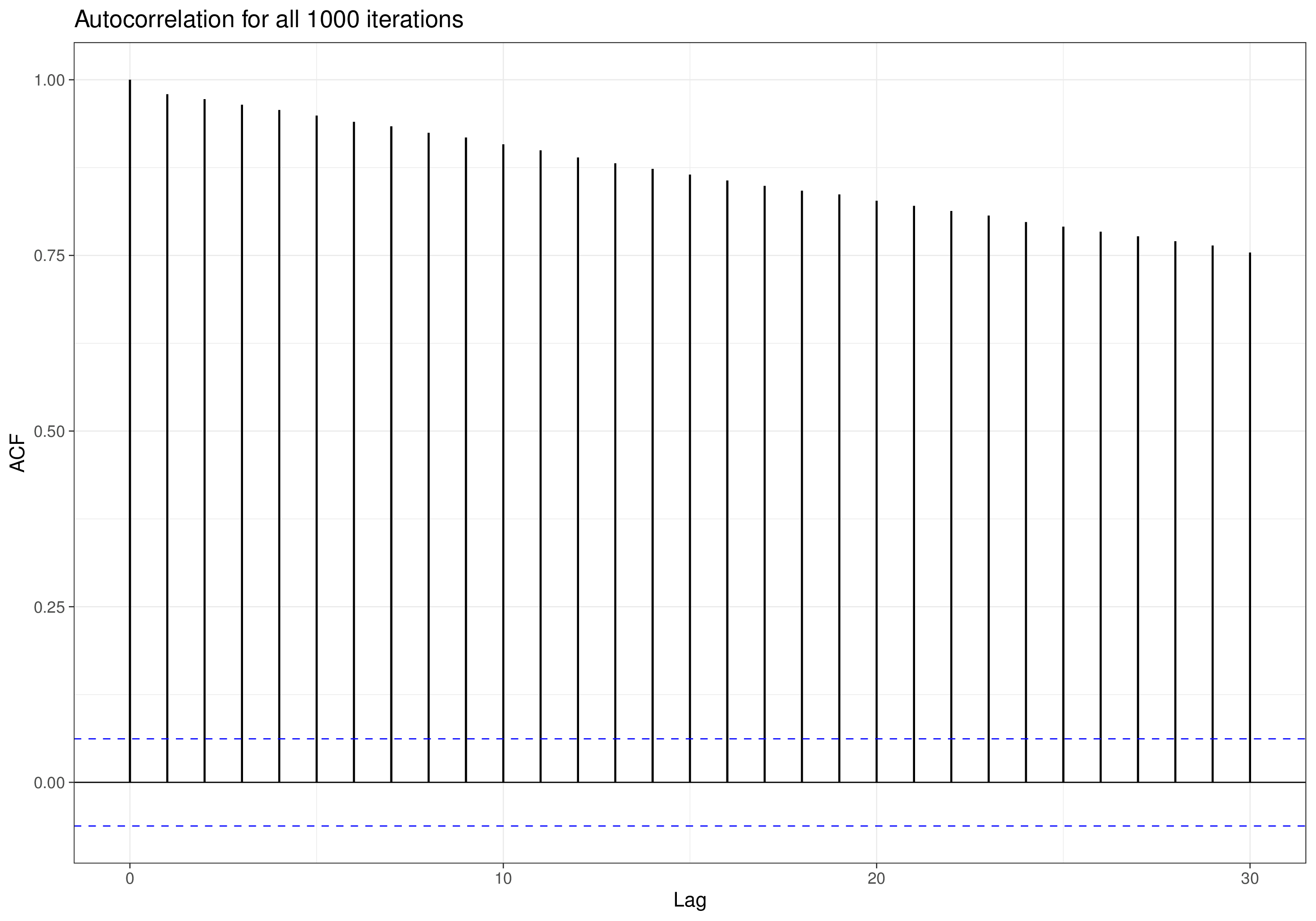
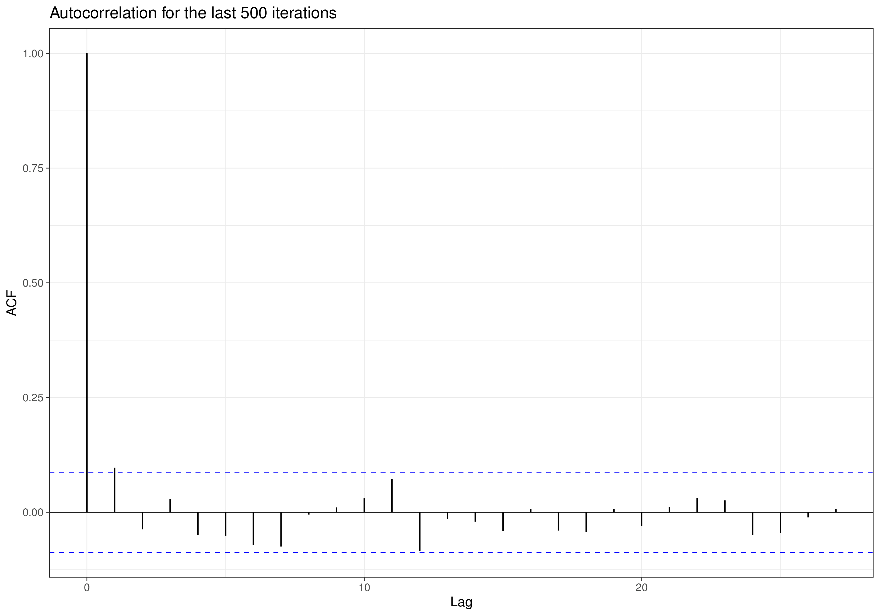
As is possible to see, when we select the whole sample of 500 iteration per chain (so 1000 in total), as in Figure 2.14 (a), the level of autocorrelation is large, even for large values of the lag: values \(l=1,\ldots,L\) along the \(x\)-axis indicate that we are considering the correlation between iterations that are \(l\) places apart. If things have worked, the level of autocorrelation should be reasonably small, even for small lags – this is clearly not the case in Figure 2.14 (a), when even at lag \(l=30\) correlation is around 0.75.
If we instead restrict the sample to the final 250 per chain (so 500 in total), things are much better – for the whole range of lags depicted in Figure 2.14 (b), the value of the correlation among iterations is much smaller and contained within a margin of Monte Carlo error (indicated by the horizontal dashed lines).
How many MCMC iterations should I use?
One of the critical questions in any MCMC procedure is about the size of the Markov chain sample to be used for the Monte Carlo estimation of the relevant quantities. As suggested above, ideally, we want \(n_{\text{\textit{eff}}}\) to be as close as possible to the nominal sample size \(S\), which indicates that the level of autocorrelation is minimal, thus leading to a MCMC sample that contains sufficient information. Raftery and Lewis (1995) suggest to get 95% posterior quantiles with true 94.5-95.5% coverage we typically need ESS \(> 4000\).
On the other hand, almost invariably, the default choice is for \(n_{\text{\textit{sims}}}=1000\) simulations. Historically, 1000 was a large enough, round-looking number, which would nicely balance the need for representativeness (which increases with the number of simulations) and the computational performance (which, in the 1990s was much less powerful than it is today, on a standard machine).
In very many applications, keeping 1000 simulations after convergence and using these to get the relevant estimates is probably sufficient – some of the examples we consider in the next chapters use exactly this strategy. But the choice of \(n_{\text{\textit{sims}}}=1000\) after convergence should not be made dogmatically.
One important metrics to consider is the Monte Carlo Standard Error (MCSE), computed as the ratio of the standard deviation of the MCMC simulations to the effective sample size. So for a generic vector of \(S\) simulations \(\left(\theta^{(1)},\ldots,\theta^{(S)}\right)\), the MCSE is \[\text{MCSE}(\theta) = \frac{\text{sd}\left(\theta^{(1)},\ldots,\theta^{(S)}\right)}{\sqrt{n_{\text{\textit{eff}}}}}\] and it is a measure of how accurate the posterior mean is (Kruschke, 2015).
In the example shown above, we can compute the MCSE for the simulations stored in the object x by taking the standard deviation of the two chains stacked up as a vector and then dividing by \(\sqrt{n_{\text{\textit{eff}}}}\), which gives values of 24.343 and 0.34981, respectively.
Another helpful advice is to test the stability of the estimates (cfr. Figure 1.8), upon varying the length of the MCMC sample. This is generally helpful, because we may not have a good idea of how slow the process will be and thus we may start with a short run (to sort of “test the water”), then produce a longer sample and then may an even longer still. Comparing the resulting estimates may give us an indication of whether any marginal improvement is worth it – if the estimates do not vary very much, we are probably fine to stop.
Centring and thinning
When substantial autocorrelation is present, we have several options to try and mitigate it. Often, the best idea is to try and reparameterise the model – for instance, in a regression model \[\begin{eqnarray*} y_i & \sim & \text{Normal}(\mu_i,\sigma)\\ \mu_i & = & \alpha + \beta x_i, \end{eqnarray*}\] the posterior distributions for the two regression coefficients \((\alpha,\beta)\) tend to be highly correlated, which in turns slows down convergence. One easy and efficient way around it is to reparameterise the linear predictor as \[\mu_i = \alpha^* + \beta^*(x_i -\bar{x}),\] i.e. by considering the centred version of the covariate (see Section 2.4.7 of Baio, 2012). This changes the scale of the intercept \(\alpha^*\), but helps break the correlation among the coefficients, thus improving convergence.
An alternative to model reparameterisation is to use “brute force”, i.e. run the model for a much longer time – there are theorems to ensure that if \(S\rightarrow \infty\), convergence is guaranteed. Other than the computational effort, this has, possibly, some implications in terms of computer memory – if we run an MCMC process for, say, twenty parameters and for 1 000 000 iterations after a burn-in of 10 000 iterations, then we would be storing in the computer memory a very large object.
To limit this issue we can use thinning – this amounts to running the process for longer (which is what makes the actual difference), but only retaining one in every \(T\) simulations. The resulting sample that we save for the MC analysis is thus shorter than the actual number of simulations, which makes it more manageable. See the example discussed in Section 3.3 for more details.
Example 2.8. Semi-conjugated model (continued): convergence. As this model is semi-conjugated, convergence is not really an issue. However, to demonstrate this, we replicate the MCMC process shown in Example 2.7, using two different sets of starting points. We can do this using the following R code.
# Wrap up the MCMC code into a function; Takes the number of simulations
# as input, with default arbitrarily set at 1000
gibbs=function(nsim=1000) {
  for (i in 2:nsim) {
      sigma_n=sqrt(1/(1/sigma2_0 + n/sigma2[i-1]))
      mu_n=(mu_0/sigma2_0 + n*ybar/sigma2[i-1])*sigma_n^2
      mu[i]=rnorm(1,mu_n,sigma_n)

    alpha_n=alpha_0+n/2
    beta_n=beta_0 + sum((y-mu[i])^2)/2
    tau[i]=rgamma(1,alpha_n,beta_n)
    sigma2[i]=1/tau[i]
  }
  sigma=sqrt(sigma2)
  # Saves the output to a list
  list(mu=mu,sigma=sigma)
}

# Create a list object in which we will store the results
sims=list()

# First set of initial values
mu=tau=numeric()
sigma2=1/tau
mu[1]=rnorm(1,0,3)
tau[1]=runif(1,0,3)
sigma2[1]=1/tau[1]
# Run the MCMC algorithm and save the output in the first element of 'sims'
sims[[1]]=gibbs(5000)

# Then selects different initial values
mu=tau=numeric()
sigma2=1/tau
mu[1]=rnorm(1,10,3)
tau[1]=runif(1,5,10)
sigma2[1]=1/tau[1]
# Re-run the MCMC algorithm, saving the output in the second element of 'sims'
sims[[2]]=gibbs(5000)
Because the algorithm is quite cheap, computationally, we simulate \(n_{\text{\textit{sims}}}=5000\) iterations in each chain, which we can use to assess convergence. For instance, we can use the function Rhat() defined above and apply it to a matrix with two columns (each a vector of simulations for either mu or sigma from the two MCMC chains), to compute \(\hat{R}\).
# Uses the function Rhat() to compute the PSR for 'mu' and 'sigma'
Rhat(cbind(sims[[1]]$mu,sims[[2]]$mu))
[1] 0.9999104Rhat(cbind(sims[[1]]$sigma,sims[[2]]$sigma))[1] 0.9999196For both variables, the value of \(\hat{R}\) is extremely close to 1, indicating that convergence is achieved. This is also confirmed by the visual inspection of the two traceplots, shown in Figure 2.15. Again, as the model is semi-conjugated, even starting from very different initial values, the two chains converge immediately.
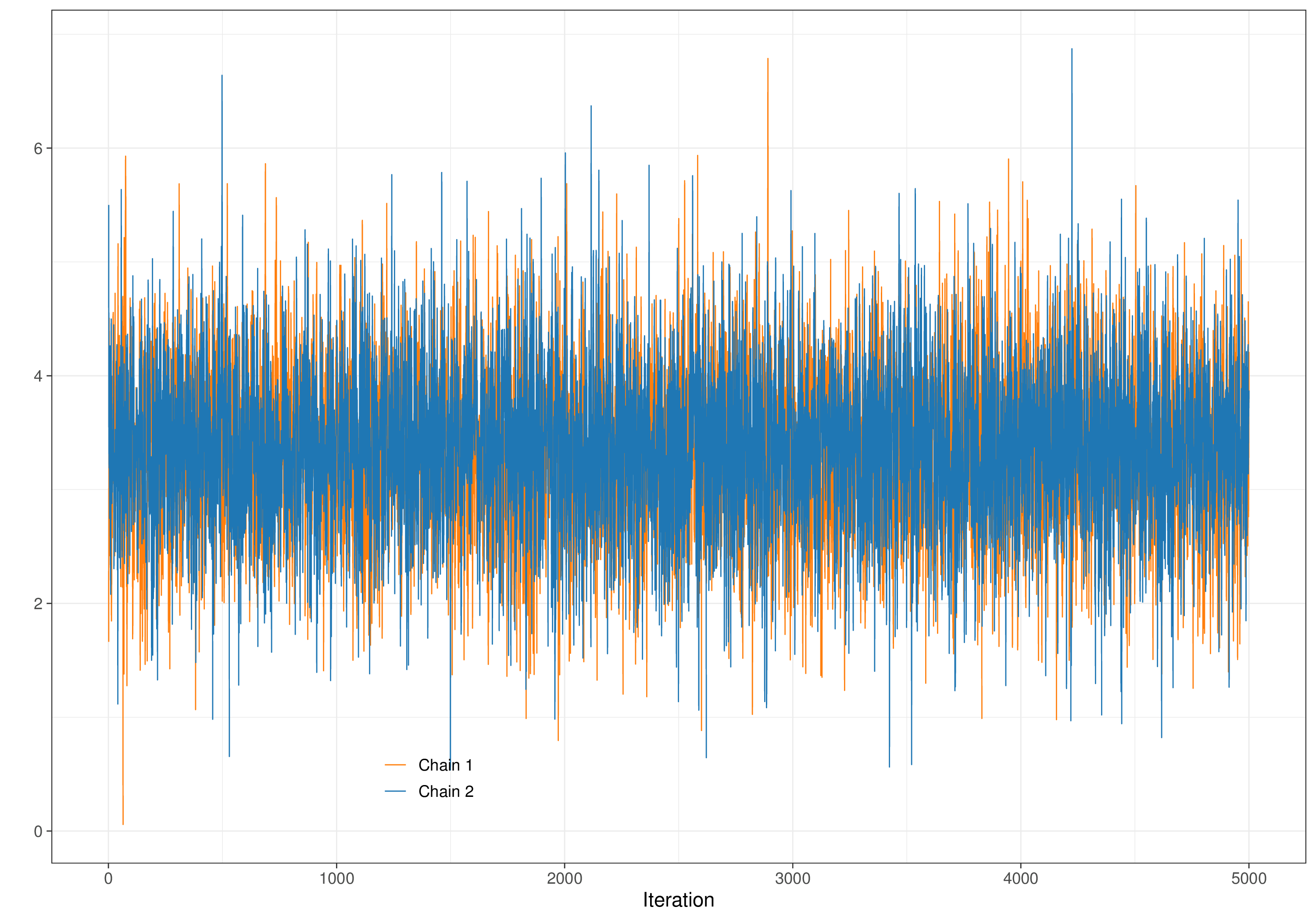
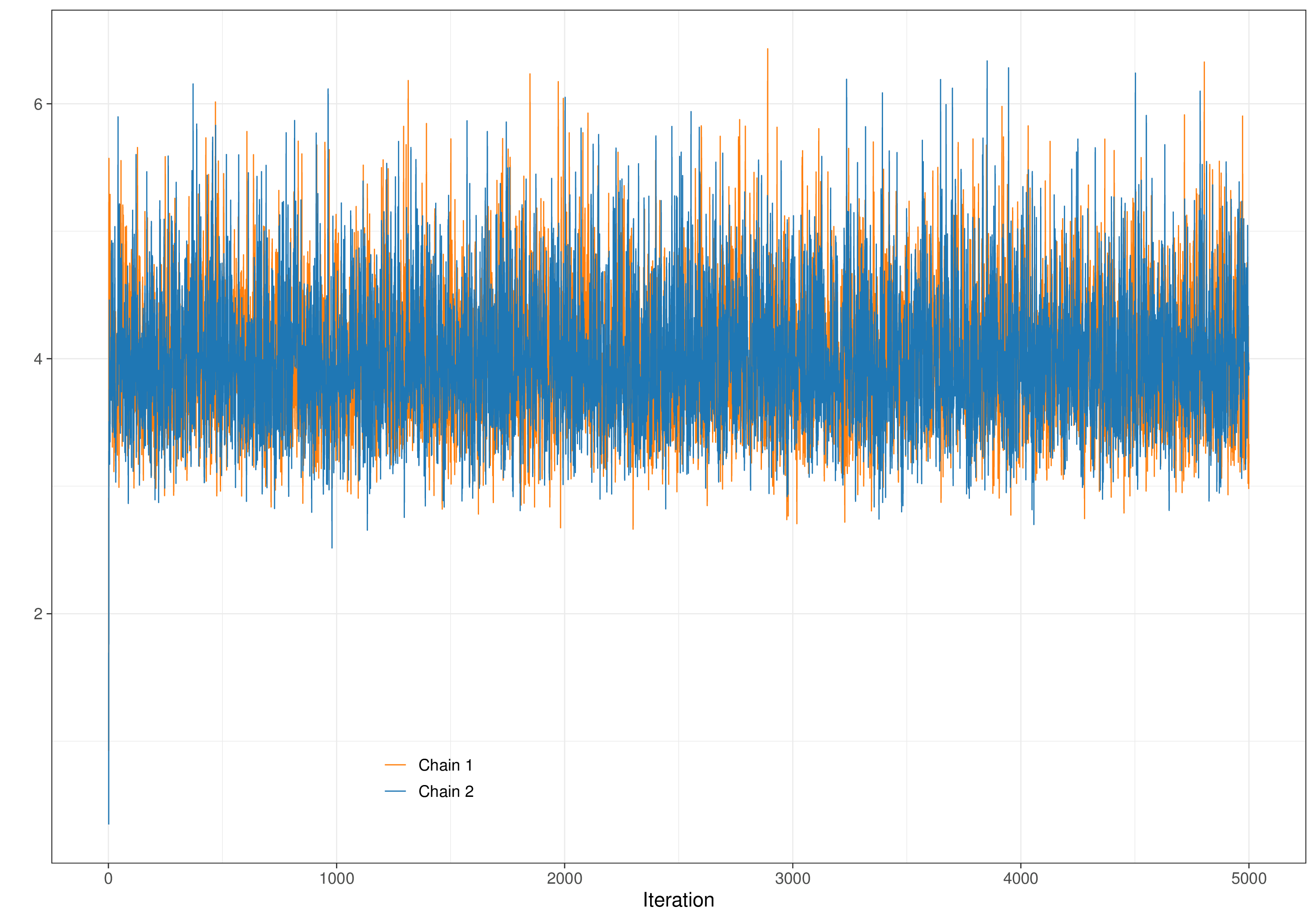
If we apply Equation 2.14 we can also compute \(n_{\text{\textit{eff}}}=10000\) for both \(\mu\) and \(\sigma\). In this case, the combination of a large MCMC run and the fact that the model is semi-conjugated implies that for all parameters the ESS this coincides with the nominal sample size.
2.3.3 Hamiltonian Monte Carlo
Hamiltonian Monte Carlo (HMC – see Betancourt, 2018; Neal, 2011; Gelman et al., 2013; Kruschke, 2015) is another important MCMC algorithm, which has recently gained popularity. HMC is based on the physical concept of Hamiltonian dynamics, which can be used to model the idealised situation of a frictionless particle sliding over a surface of varying slope.
In a nutshell, HMC is an extension of simpler MCMC algorithms such as the Metropolis-Hastings, which are based on random walks through the parameter space, where successive moves are derived from a proposed symmetrical distribution (centred around the current parameter position) and accepted or rejected, depending on the relative density of the target (posterior) at the current parameter value.
The main innovation of HMC is that, to determine the next state of the parameters, it uses a proposal distribution that does not need to be symmetrical. In addition – and crucially – this proposal distribution changes depending on the current value of the model parameters. This makes the process highly adaptive and particularly efficient in cases where the number of parameters is very large.
Intuitively, we can think of HMC as a smart explorer navigating a rugged terrain whose height represents the (negative log-)density associated with different parameter values. The explorer uses information about the gradient of this density to guide its movement, allowing it to traverse the terrain more efficiently and sample from the distribution more effectively.
The classic analogy used to explain HCM is that of a marble travelling on a slope: the original position is generated randomly and the marble is given a random flick, to gain initial momentum. As shown in Figure 2.16, if the marble is in an area of low probability or, equivalently, high “potential energy” (i.e. the negative log-density), then it will tend to slide more quickly down the slope and will retain higher momentum before eventually stopping. If, on the other hand, it sits at the bottom of the valley (i.e. the area of highest density), the flick will have to be much stronger to make it climb over the hills.
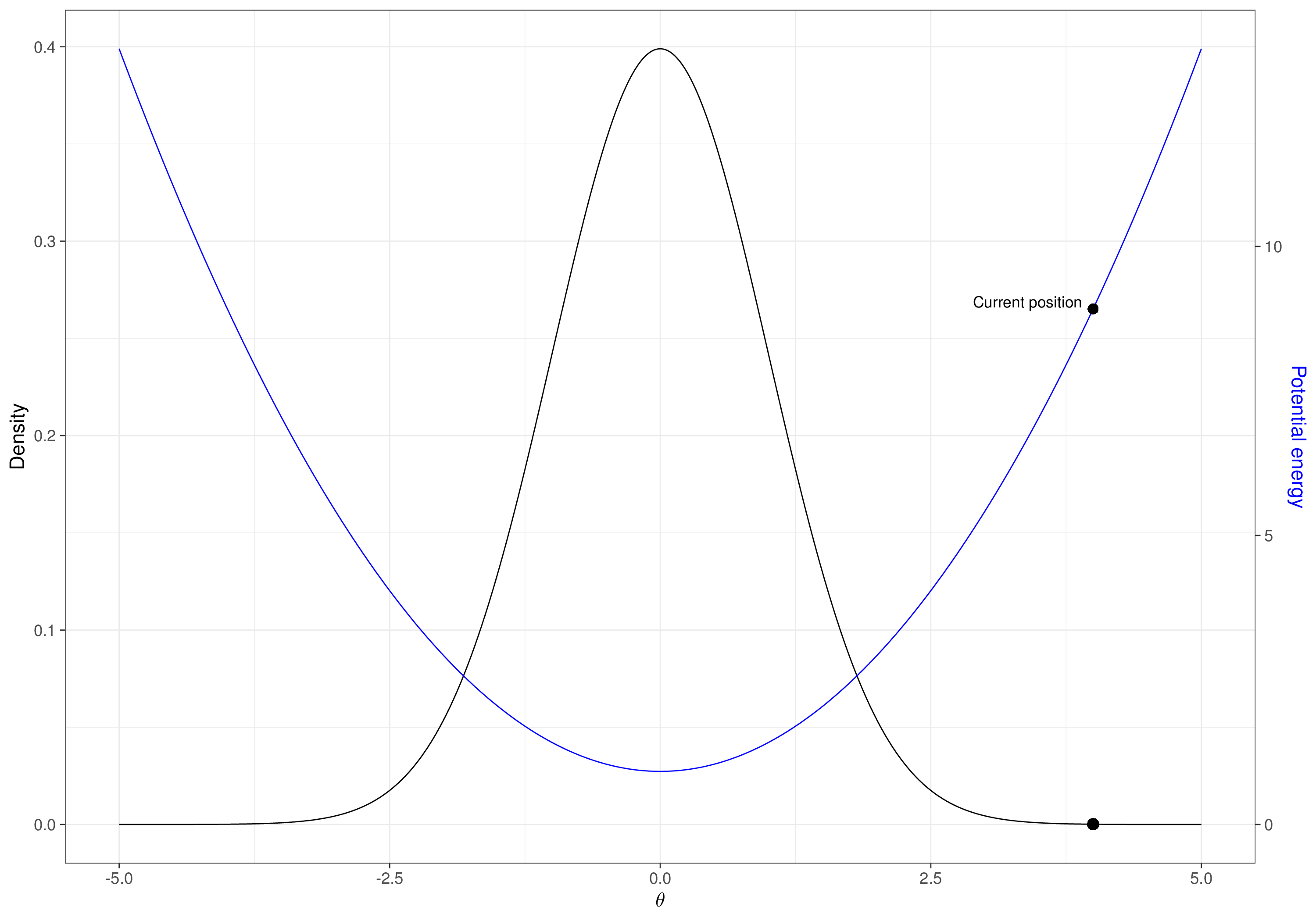
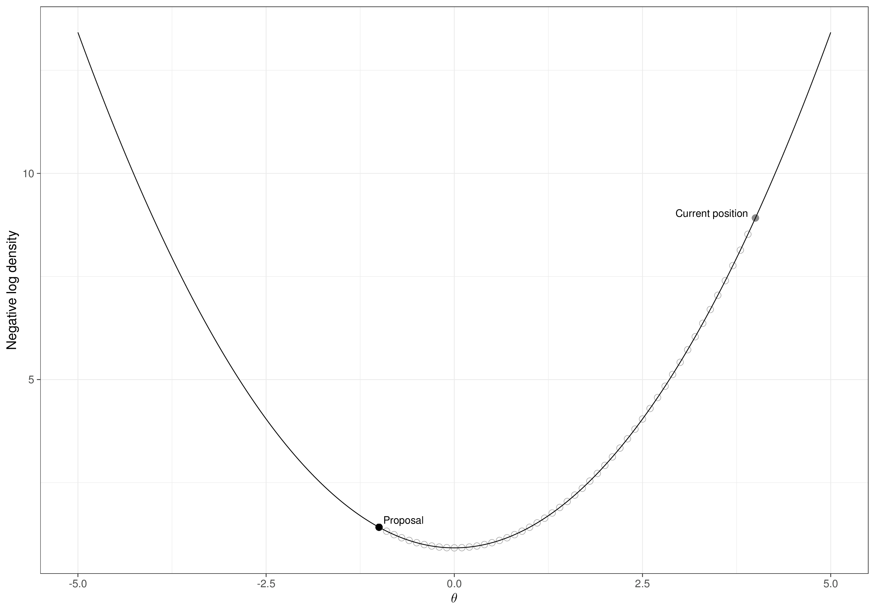
The main idea is that, using complex Hamiltonian dynamics (based on differential equations) to approximate the physical movements of the marble, a single iteration of HMC involves letting the marble slide up and down the potential energy function for a set number of discrete times, at the end of which the new position is proposed. This is then subjected to a Metropolis-like acceptance step.
By using information about the gradient of the target distribution to propose more informed moves, HMC is able to explore the space more effectively and sample from the target distribution more efficiently. This is particularly true in high-dimensional spaces and for sampling from distributions with complex geometries or strong correlations, where traditional MCMC methods may struggle.
NoteHMC vs Gibbs sampling
Generally speaking, HMC can be more computationally efficient than other MCMC schemes (including Gibbs sampling) because of the following features.
- Exploration of high-dimensional spaces. HMC incorporates information about the geometry of the target distribution through Hamiltonian dynamics, allowing it to move more effectively through the space and explore distant regions in fewer steps. In contrast, Gibbs sampling updates each parameter individually, which can be less effective in high-dimensional spaces due to slow mixing.
- Adaptive proposals. HMC can adaptively tune the proposal distribution during sampling by adjusting its defining features based on the local geometry of the target distribution. This adaptability can lead to more efficient exploration of complex distributions with varying scales and correlations. Gibbs sampling, on the other hand, generates samples based on the full conditionals for each parameter, which may not always be optimal for efficient exploration.
- Handling correlated variables. HMC is better suited for sampling from distributions with strong correlations among the parameters. By using Hamiltonian dynamics to propose joint updates of the parameters, HMC can more effectively traverse the parameter space and capture dependencies between variables. In Gibbs sampling, updates are made independently for each parameter, which may result in slower convergence when dealing with correlated variables.
- Computational efficiency. While HMC involves additional computational overhead due to the simulation of Hamiltonian dynamics and the need for gradient calculations, it can be more computationally efficient in high-dimensional settings compared to Gibbs sampling. This efficiency is especially pronounced when the target distribution exhibits complex geometric structures or strong correlations, as HMC can exploit this information to propose more effective moves in the parameter space.
In reality, in the majority of applications of Bayesian modelling to HTA problems (as presented in the rest of this book), there are only marginal gains in using the more complex HMC structure.
With the notable exceptions of highly structured hierarchical models (as those arising in the cases shown in Chapter 6 and more specifically in Chapter 11) and survival analysis (Chapter 8), Gibbs sampling is typically sufficient to fully and efficiently explore the target posterior distribution in which we are interested in the HTA context.
For this reason, we have presented here only a sketch of the main features of HMC – but refer the reader to, for example, Stan development team (2024), Kruschke (2015) or McElreath (2015) for more detailed and yet accessible descriptions.
2.4 Conclusions
This chapter has presented the process of Bayesian computation, with a view of combining background or contextual information (in the form of a prior distribution) with evidence from data, into a full posterior distribution. We have looked at ways in which we can define the prior distribution, aiming at not excerpting undue sensitivity on the final inference, but also allowing the inclusion of genuine information into the model.
We have also described in detail the basics of Markov Chain Monte Carlo algorithms (specifically the Gibbs sampling), which are used to make Bayesian inference. This process requires careful post-processing to ensure that the results are sensible and we have provided several diagnostic measures and a workflow to use in practice.
In the next chapter, we showcase specific software that can be used to make Bayesian inference. We consider JAGS as the software of choice throughout most of this book and we discuss in details the setup and machinery necessary to run Bayesian models.
Interestingly, Fienberg (2006) notes that the principle of insufficient reason was not the one guiding Bayes in his original formulation, which was rather based on physical properties of the marginal distribution for the observed data.↩︎
Assuming that the standard deviation is known without uncertainty is of course a gross, but not entirely uncommon simplification – see for instance Example 1.1.↩︎