8 Survival analysis in HTA
8.1 Introduction
Survival modelling is a cornerstone of biostatistical analysis, specifically designed to model time-to-event outcomes, such as the overall time between the beginning of an observation or exposure (e.g. diagnosis of cancer) until a relevant event (typically death, or progression to a different health state). This represents a powerful analytic framework that provides much more granular information than cruder binary (event vs no-event) analyses, thus enabling the estimation of richer output, including instantaneous and cumulative risks, over time.
In typical biostatistics applications, survival modelling is used to understand the magnitude of treatment effects and identify prognostic factors, accounting for the data-generating mechanism. In the context of HTA, it also plays a pivotal role, because decisions are made at the population level and often require extrapolation beyond the follow-up observed in clinical studies. Accurate survival estimates are therefore essential not only for quantifying treatment effectiveness but also for projecting downstream costs, quality-adjusted life years and overall cost-effectiveness.
Whenever possible, modelling at the individual-level allows the incorporation of patient heterogeneity, adjusting for covariates and the propagation of uncertainty that can then inform robust evidence-based policy decisions. This makes survival analysis both a statistical and an economic tool, bridging clinical evidence with the long-term evaluations required for health system decision-making.
While the overall methodology is well established, its application in HTA does have some specific quirks, which are deeply related to the nature of the available data, as well as the fundamental focus on decision-making, rather than simple inference. For these reasons, which we explore in details below, survival methods applied in HTA are often “non-standard”, in comparison to those used in “biostatistical” modelling. Despite the underlying complexity, survival analysis is extremely prevalent in HTA, because it is the natural modelling framework for cancer studies, which represent a large proportion of all the HTA appraisals (Latimer, 2011).
In this chapter, we provide a general framework for survival analysis, specifically for HTA and focus on a number of “typical” distributional assumptions, as well as on computational methods that are particularly efficient for this type of outcome. Jackson et al. (2025) provide a wider introduction (with larger focus on non-Bayesian modelling), while aspects of HTA modelling related to survival analysis are also presented in Dias et al. (2018, chap. 10) and in Sharples and Demiris (2020).
NoteNotation for survival modelling
As suggested in Note 4.1 in Section 4.2, throughout this chapter we slightly modify our general notation, in which we have used the symbol \(t\) to index the treatments under consideration.
In order to align with the general survival analysis literature (and because, hopefully, there is no major confusion with the rest of the book), in this chapter, we indicate with \(t_i\) the main outcome of the analysis, i.e. the time until a relevant event happens for individual \(i\).
We also use throughout this chapter the index \(k=1,\ldots,K\) to indicate relevant parts of the models, as in Equation 8.8, or in Equation 8.13.
8.2 General framework for survival analysis
The general modelling framework for time-to-event, can be described as follows. The main outcome is the observed time at which the event under study is recorded for the \(i-\)th individual, \(t_i\). We can describe the sampling variability in the observed times using a density \(f(t_i\mid \boldsymbol\theta)\), as a function of a set of relevant parameters.
In addition, we can consider a number of helpful quantities to describe the survival mechanism: the first and, perhaps, most important is the survival function \[ S(t\mid\boldsymbol\theta) = \Pr(T>t) = 1-F(t\mid\boldsymbol\theta) = 1 - \int_0^t f(u\mid\boldsymbol\theta)du, \] where \(F(t\mid\boldsymbol\theta)\) is the cumulative density of the variable \(T\). The survival function describes the probability of an individual surviving beyond time \(t\).
Other important quantities are the hazard function \[ h(t\mid\boldsymbol\theta) = \lim_{dt \rightarrow 0}\frac{\Pr(t\leq T < t+dt \mid T\geq t)}{dt}, \tag{8.1}\] which quantifies the instantaneous risk of experiencing the event, as well as the related cumulative hazard function \[ H(t\mid\boldsymbol\theta)=\int_0^t h(u\mid\boldsymbol\theta) du. \]
NoteBrothers and sisters
By their mathematical properties, we can retrieve a set of useful relationships that allow us to connect \(F(\cdot)\), \(S(\cdot)\). \(f(\cdot)\), \(h(\cdot)\) and \(H(\cdot)\). Thus, specifying one of them is sufficient to fully characterise the survival model.
By definition, the density function is the derivative of the cumulative function, with respect to the time variable \[\displaystyle f(t\mid\boldsymbol\theta)=\frac{d}{dt}F(t\mid\boldsymbol\theta)=F^\prime(t\mid\boldsymbol\theta). \tag{8.2}\]
As the numerator of Equation 8.1 is a conditional probability, it can be factorised into the ratio of the joint to the marginal probabilities (see Section 5.2.2) and thus \[ \begin{aligned} h(t\mid\boldsymbol\theta) & = \lim_{dt \rightarrow 0}\frac{\Pr(t\leq T < t+dt,T\geq t)}{\Pr(T\geq t)dt} = \lim_{dt \rightarrow 0}\frac{\Pr(t\leq T < t+dt)}{S(t\mid\boldsymbol\theta)dt} \\ & = \frac{f(t\mid\boldsymbol\theta)dt}{S(t\mid\boldsymbol\theta)dt} = \frac{f(t\mid\boldsymbol\theta)}{S(t\mid\boldsymbol\theta)}, \end{aligned} \tag{8.3}\] because, obviously, the probability that \(T\) is in the interval \([t; t+dt)\) and, at the same time, \(T\geq t\) is just \(\Pr(t\leq T < t+dt)\); and, by definition, \(f(\cdot)dt\) is the probability that the variable \(T\) is in a small interval of width \(dt\).
Combining the definition of the survival function and Equation 8.2, its derivative with respect to the time variable is the negative of the density function \[\displaystyle S^\prime(t\mid\boldsymbol\theta)=\frac{d}{dt}S(t\mid\boldsymbol\theta)=\frac{d}{dt}\left[1-F(t\mid\boldsymbol\theta)\right]=-f(t\mid\boldsymbol\theta). \tag{8.4}\]
Combining Equations 8.3 and 8.4, the hazard function can be represented as the ratio of the derivative to the actual survival function \[\displaystyle h(t\mid\boldsymbol\theta)=-\frac{S^\prime(t\mid\boldsymbol\theta)}{S(t\mid\boldsymbol\theta)}. \tag{8.5}\]
Given Equations 8.1 and 8.5, as well as the basic properties of differential calculus, the cumulative hazard function can also be expressed also as the negative log-survival \[\displaystyle H(t\mid\boldsymbol\theta)=\int_0^t -\frac{S^\prime(u\mid\boldsymbol\theta)}{S(u\mid\boldsymbol\theta)}du=-\log(S(t\mid\boldsymbol\theta)). \tag{8.6}\]
8.2.1 Censoring
Another important defining feature of time-to-event data is the fact that, almost invariably, the evidence in the observed data is limited. This is because, most often, the length of the follow-up is not enough for us to be able to observe the event under study on all the individuals involved – a phenomenon typically referred to as censoring1.
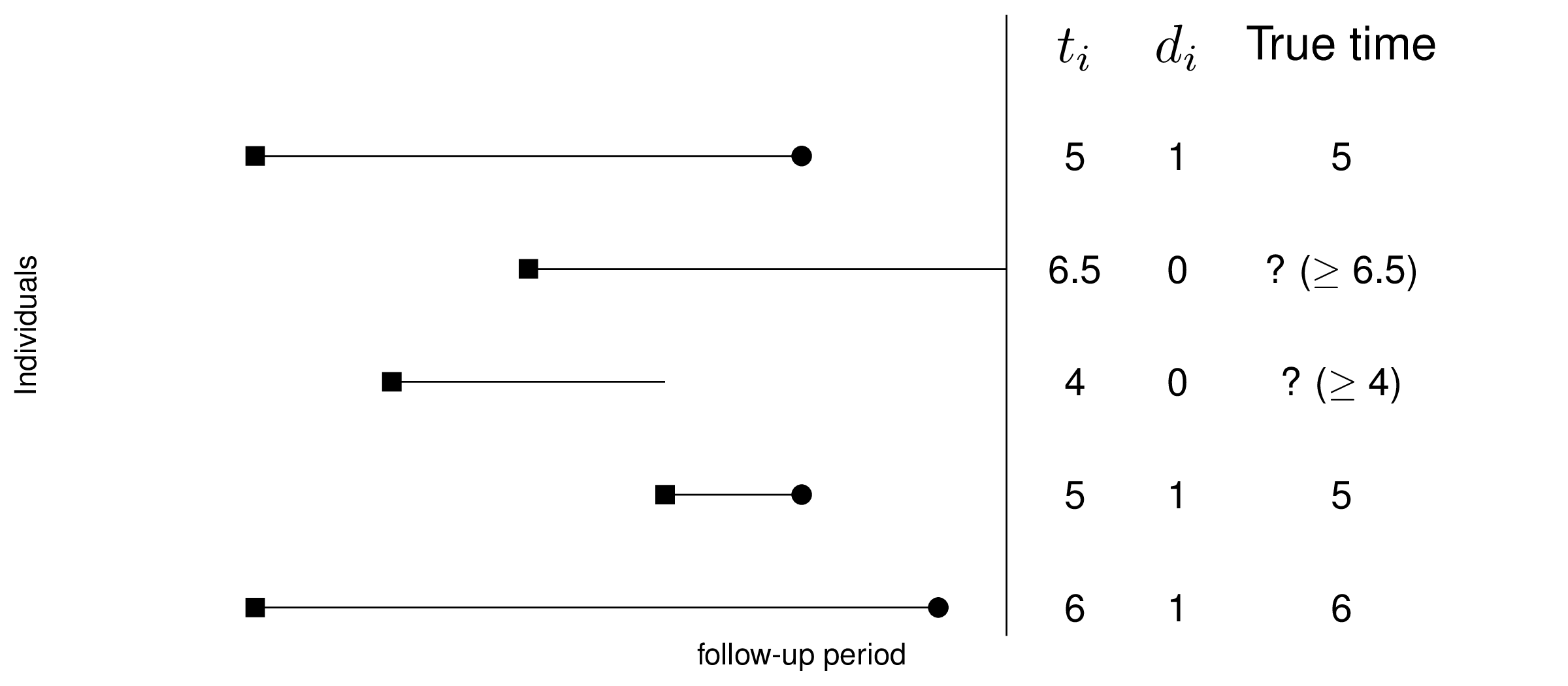
Thus, in addition to the observed times \(t_i\), we usually consider an event indicator \(d_i\) (for “dummy” variable), taking value 1 if the event actually happens within the time horizon during which the data are observed, or 0 when the \(i-\)th individual is “censored”.
If \(d_i=1\), then \(t_i\) is fully observed; conversely, if \(d_i=0\), we do not know whether the event actually occurs – it may in the future, but we just do not have this information. Consequently, when \(d_i=0\), then the observed \(t_i\) does not represent the true “survival time”. Figure 8.1 depicts this by showing that for some individuals the entire history is known, while for others, key information (e.g. whether the event is actually occurred) is not available.
Censoring is important, because just like missing data (see Chapter 10), it implies that the information present in the data is not complete. Consequently, in the presence of censoring, the individual contribution to the likelihood function is expressed as \[ \mathcal{L}(\boldsymbol\theta\mid t_i,d_i) = h(t_i\mid\boldsymbol\theta)^{d_i} S(t_i\mid\boldsymbol\theta). \tag{8.7}\] Basically, if the individual is not censored (i.e. they have survived up to \(t\) and hence \(d_i=1\)), their risk of experiencing the event is simply described by the full density function, expressed as \(h(t_i\mid\boldsymbol\theta) S(t_i\mid\boldsymbol\theta)\) – see Equation 8.3; if, on the other hand, they are censored (i.e. \(d_i=0\)), then their risk is measured by the survival function as the probability that they will experience it in the future (after time \(t\)).
Equation 8.7 can be used (typically taking the log, for computational stability) to perform calculations on the density \(f(\cdot)\) – we return to this point in Section 8.3.4.
8.3 Survival analysis in HTA
In typical applications of survival analysis, e.g. in the context of randomised clinical trial, the main objective of the statistical analysis is to estimate the impact of a number of covariates (including the treatment arm) on the survival time. This sort of structure is applied specifically for cancer drug trials. In these cases, typically, the analysis is focused on a head-to-head comparison between a new intervention (e.g. a new cancer drug) and some sort of standard of care (e.g. chemotherapy).
In the case of survival modelling in HTA, there are at least two added complications that must be carefully taken into account.
8.3.1 Extrapolation
Almost invariably, the nature of these studies implies a time horizon that does not allow to follow-up all the individuals enrolled until they experience the event of interest (usually, sadly, death), through the effect of censoring and other considerations (e.g. treatment switching for lack of efficacy – see for instance Latimer et al., 2016).
Figure 8.2 (a) shows the typical representation of trial data in the form of Kaplan-Meier (KM) curves (Kaplan and Meier, 1958) – see Note 8.1 below for more technical details. These are non-parametric estimators for the probability of survival at any given time point over the duration of the follow-up in a study and are shown as the step curves (surrounded by a non-parametric 95% interval estimate). KM estimates are ubiquitous in survival analysis, as they are a very efficient way of summarising the observed data.
Alongside the KM curves for the two treatment arms (generically labelled as “Control” and “Intervention”), we have included two smooth curves, fitted to the observed data to estimate survival over the observed study period. The two dots on the smooth curves indicate the estimated median survival time, i.e. the point along the \(x\)–axis in correspondence of the value of 50% along the \(y\)–axis.
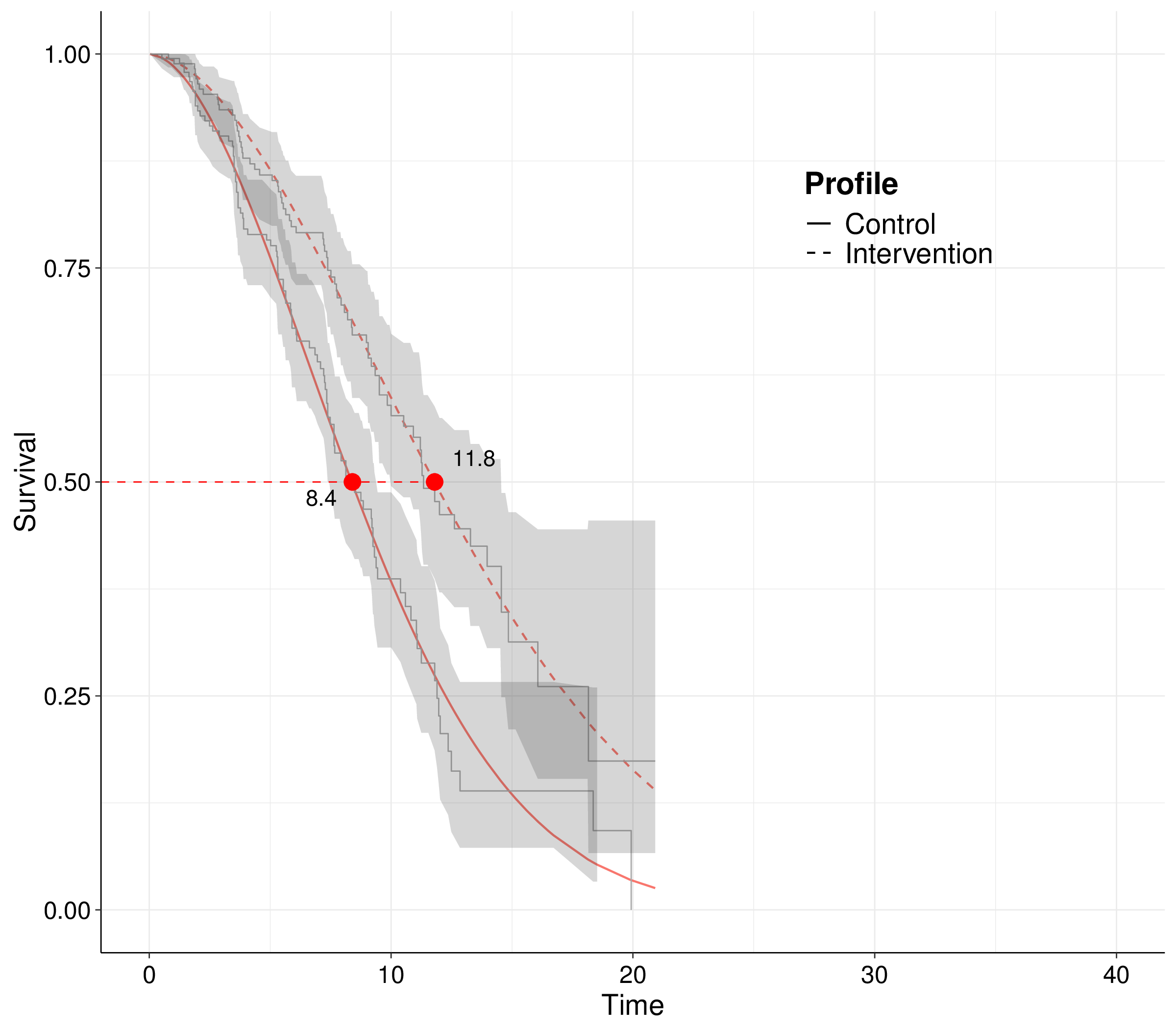
In typical survival studies, the median time is one of the quantities of interest because, as shown in Figure 8.2 (a), we do not have enough observations to be able to estimate the survival curves all the way down to 0, i.e. at the point when all the observed individuals actually experience the event. Notice that in the case depicted in Figure 8.2 (a), censoring is actually not too extreme, as indicated by the fact that both curves are reasonably close to 0 (especially for the controls). Nonetheless, for the intervention arm, there is about 15% of individuals for whom we do not know the time at which the event (death) occurs and hence both the KM and the smooth curve end abruptly at the end of the follow-up time.
This is in contrast with the needs of the HTA analysis: we cannot just rely on the difference we measure in the study period, e.g. in this case a treatment effect of 11.8 \(-\) 8.4 = 3.4 units of time, say months, in terms of median survival. That is because the economic analysis must take a “life-time horizon”: if a treatment is approved for reimbursement, it will be provided to individuals for as long as they need it and the effects must then be measured in terms of mean, rather than median survival time.
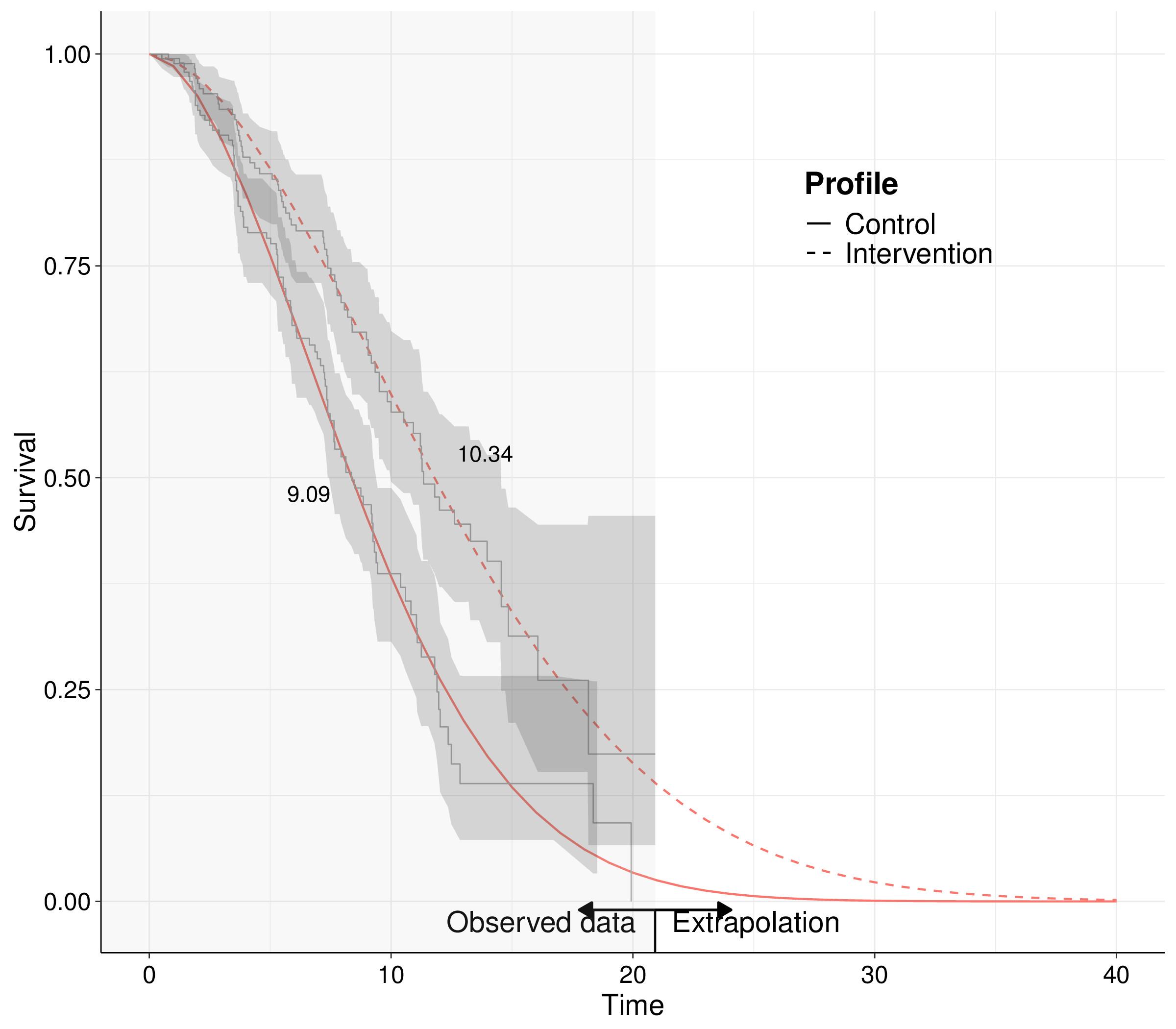
Figure 8.2 (b) shows this by expanding the smooth curve beyond the duration of the observed times – this is typically referred to as extrapolation. By expanding the time horizon to, in this particular case, over 40 units of time, we ensure that the survival curves go down to 0, to the point where all the individuals will have experienced the event under study. This is necessary because, integrating by part and using Equation 8.4, we can prove that the mean survival time is equivalent to the full area under the survival curve: \[ \text{E}[T] := \int_0^\infty t f(t\mid\boldsymbol\theta)dt = \int_0^\infty S(t\mid\boldsymbol\theta) dt. \]
Importantly, if we are able to extrapolate the survival curve over a longer time horizon, the treatment effect may vary even substantially: in the case of Figure 8.2 (b), it is 10.34 \(-\) 9.09 = 1.25 units of time, in terms of mean survival – that is basically half the median treatment effect that we get from the trial data with no extrapolation.
There are two main obvious implications of this issue. Firstly, in HTA it is harder to apply standard modelling for survival analysis, such as Cox Proportional Hazard models (Cox, 1972). This is because, while they have the great advantage of not committing to a fully parametric specification for the time-to-event variable, their semi-parametric nature makes it harder to produce time-quantile predictions, e.g. extrapolate the survival curves.
For this reason, in HTA we tend to rely more heavily on parametric models for survival analysis, which do require more explicit assumptions. Therefore, the way in which we produce this extrapolation beyond the observed trial data becomes crucial and may exert notable sensitivity to the overall economic results (Latimer, 2011).
Note 8.1: Kaplan-Meier estimates
Imagine we have a fictional dataset recording the time-to-event for \(n=10\) individuals, as \(\boldsymbol{t}=( 0.03,0.03,0.92,1.48,1.64,1.64,1.7,1.7,1.74,1.77 )\). The data can be aggregated by listing the unique times at which events happen and counting the progression of individuals from being “at risk” (i.e. exposed to the risk of the event) to having actually experiencing it. Table 8.1 shows this aggregation.
| Time | At risk | Events | Survivors |
|---|---|---|---|
| 0.00 | 10 | 0 | 10 |
| 0.03 | 10 | 2 | 8 |
| 0.92 | 8 | 1 | 7 |
| 1.48 | 7 | 1 | 6 |
| 1.64 | 6 | 2 | 4 |
| 1.70 | 4 | 2 | 2 |
| 1.74 | 2 | 1 | 1 |
| 1.77 | 1 | 1 | 0 |
The KM estimator for the survival curve is formally defined as \[ S^{\text{KM}}(t) = \prod_{i: t_i \leq t} \left(1 - \frac{m_i}{r_i}\right), \] where: \(\mathcal{R}_t = \{i: t_i \leq t\}\) indicates the risk set, i.e. the set of observed times below the index value \(t\); \(m_i\) is the total number of events observed in each of the times in the risk set; and \(r_i\) is the number of individuals at risk in each of the times included in the risk set.
In the example of Table 8.1, the survival curve for the third time (\(t=0.92\)) can be computed as \[ \begin{aligned} S^{\text{KM}}(0.92)& = \left(1-\frac{0}{10}\right)\left(1-\frac{2}{10}\right)\left(1-\frac{1}{8}\right) \\ & = 1 \times \frac{8}{10} \times \frac{7}{8} = \frac{7}{10}. \end{aligned} \] This estimate holds until the next observed unique time – thus, in this case, we would estimate \(S^{\text{KM}}(t)=0.7\) for \(t \in [0.92;1.48)\). This gives KM estimates the typical “step-function” shape displayed in Figure 8.2 (a). Note that censoring is automatically accounted for in this computation, because the denominator is represented by the risk set, which excludes censored individuals.
8.3.2 Digitised data
One further problem with survival modelling in HTA is that, while it may be possible to access individual-level data for a specific study comparing an active (and typically innovative) treatment against some standard of care (placebo, or existing technologies, such as chemotherapy), it is very unlikely that we have available all individual-level data for all the relevant treatments, for which we may only have access to aggregated level data (cfr. Chapter 6).
Interestingly, graphical representations of the data are typically produced in the literature, in the form of Kaplan-Meier estimates, as shown in Figure 8.2 (a). Suitable algorithms exist that are able to process the image depicting the KM curves from a given study and recreate a synthetic dataset that resembles the original one, in the sense that if a KM estimated is produced using the synthetic data, the images would be very close. Zhang et al. (2024) have recently produced an R package (and a corresponding R Shiny web-application) to perform this operation, while other proprietary software, e.g. DigitizeIT or Enguage, is also available for the same purpose.
The use of digitised survival data has become increasingly popular, especially in HTA, because it allows to recreate a set of individual-level datasets that can be used to expand the full survival modelling to all the relevant comparators in an economic evaluation, effectively expanding the analysis of aggregated data. One (but not the only – we return to this point in Section 9.3.2) key limitation of digitised data is that the KM estimates are typically presented conditionally only on the treatment arm, as in Figure 8.2 (a). Every other covariate that may be of interest (e.g. sex, age, comorbidities or cancer stage at diagnosis) is averaged out in the KM curves that can be digitised. Nonetheless, this form of synthetic information is very often the only one available to modeller and thus it can be helpful, if used wisely.
In addition (and perhaps even more importantly), landmark trials upon which the evaluation of the time-to-event is based report outcomes both in terms of overall survival (OS; i.e. the time from enrolment to death) and using a surrogate progression-free survival (PFS, indicating the time from enrolment until “progression” to a worse status of prognosis). While the focus of the economic evaluation is on OS, often data from clinical experimentation are not mature enough to observe many deaths during the course of the follow-up; conversely, progression data tend to have lower amount of censoring and thus are often used as a proxy for OS – see also Green et al. (2025), who develop a model based on a Bayesian hierarchical structure similar to those discussed in Chapter 6, to “borrow” strength from the more mature PSF curves and estimate OS with increased precision.
In the case of digitised data, because the curves are presented separately, in the absence of further information, it is impossible to embed the underlying correlation in the two outcomes. In other words, in the actual dataset, there may be individuals who first progress and then die and these will contribute to both the PFS and OS curves. However, simple digitisation process will not allow us to determine who they are and effectively only generate two separate, independent datasets: one with synthetic data on the time to progression and one with synthetic data on the time to death.
Using suitable algorithms (such as the one described in Guyot et al., 2012), it is possible to correctly estimate the number of individuals at risk at different points on a time-grid, thus properly accounting for censoring. Nonetheless, the overall limitation of using digitised over fully individual-level survival data remains.
Example 8.1. NICE Technical Appraisal 174 (adapted from Williams et al., 2017). We focus here as a running example on one of NICE’s technical appraisals (TAs), specifically TA174 (NICE, 2009). This considers a full economic evaluation of rituximab in combination with fludarabine and cyclophosphamide (RFC) against fludarabine and cyclophosphamide alone (FC) for the first-line treatment of chronic lymphocytic leukaemia (CLL-8).
Although the original data used in NICE (2009), mainly based on Hallek et al. (2010), are not publicly accessible, in their tutorial on using R to model survival analysis for economic evaluation, Williams et al. (2017) make available a digitised version of the dataset, which we use as our motivating example. This version of the original dataset is also included in the R package survHE (Baio, 2020) – see Section 8.4.
Note 8.2: Digitising well is hard work…
The data presented by Williams et al. (2017) benefit from a further layer of substantive post-processing, which allowed the research team to reconstruct (a very good approximation of) the full trajectory of each individual patients.
First, the KM curves for OS, PFS and Post-Progression Survival (PPS), available from Hallek et al. (2010) have been digitised, accounting for censoring, so that there were as many times points as there were patients.
Secondly, an iterative process was performed, to keep calculating KM estimates with the generated data, until all the event and censored times were reconstructed “in the right place”, i.e. so that they matched the survival probabilities from the curves at each time to within an arbitrary margin of error of 0.005, in most cases.
The event times from the PFS and OS curves that most closely matched were assumed to be deaths without progression. This left the other PFS events as progressions and the other OS events as deaths after progression. This process is fairly straightforward in this particular study, because there are not too many deaths. The progression and death time for each individual were finally recreated by matching a progression time from the PFS curve with a time from the PPS curve that gave a death after progression time from the OS curve.
Obviously, this procedure does not retrieve the original data for all the individual trajectories with absolute certainty and therefore the digitised and post-processed dataset is merely an approximation to the “truth”.
| ID | Progression? | Death? | Progression time | Death time | Treatment |
|---|---|---|---|---|---|
| 1 | 1 | 0 | 31.991 | 32 | RFC |
| 2 | 1 | 0 | 30.552 | 30.6 | RFC |
| 3 | 1 | 0 | 27.906 | 28 | RFC |
| 4 | 1 | 0 | 2.877 | 3 | FC |
| 5 | 1 | 0 | 0.978 | 1.11 | FC |
| 6 | 1 | 0 | 1.611 | 1.77 | FC |
The data contain much information – for each individual (labelled in the ID column, in Table 8.2), we observe a treatment indicator, along two further indicators for whether progression and/or death have been observed (1) or not (0). The time (in months) at which these occur is also recorded – if either progression or death do not occur, the time is the point at which the individual is censored, i.e. they exit the observation. Because of the approximation in the digitisation and post-processing, there are some (relatively minor) discrepancies with the original data: for instance, Hallek et al. (2010) report 106 progressions in the RFC arm, while the synthetic data only count 104.
In the rest of this chapter, we consider a version of the overall dataset (which we, creatively, name data), which focuses on progression. In other words, if an individual either dies or is not observed to progress within the follow-up of the study, they are considered as censored (and the variable status is set to 0 – see Example 9.5 for more details on how to retrieve this dataset).
Figure 8.3 shows the KM curves for the two treatment arms. In the beginning and at the end of the follow-up period, there does not seem to be much separation among the two curves, when we also consider the interval estimates. In the middle of the observation period, however, the RFC arm seem to have better survival, as the KM curve is higher.
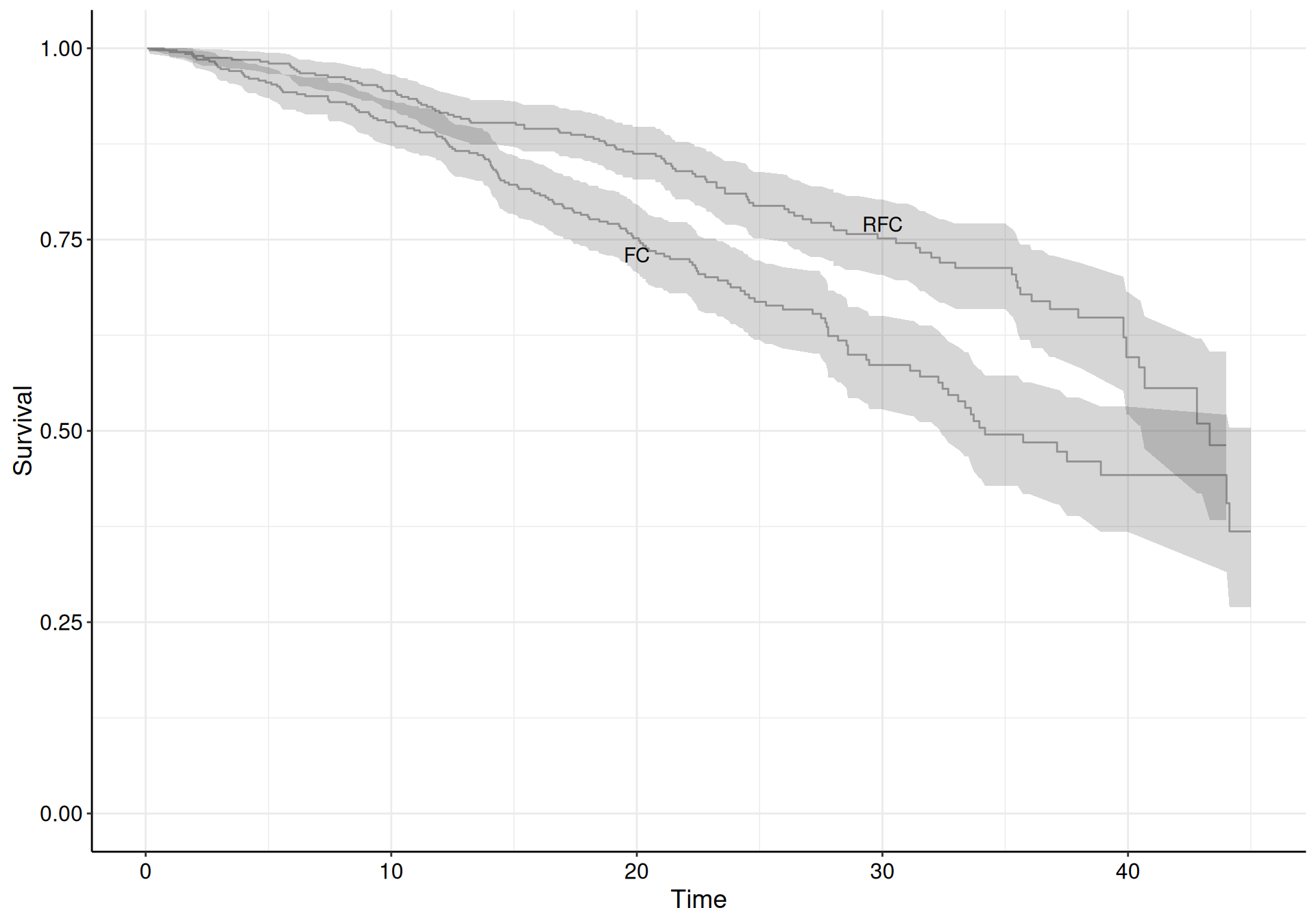
Table 8.3 shows the estimated numbers behind the KM curves. We report here, for simplicity, the first and last three times at which the estimates are produced, for both the treatment arms. In each row, we include the number of observed events (individuals who have a progression within the period defined by the two consecutive times), the overall number of individual at risk and the number of individuals censored, in that period.
| RFC | FC | ||||||
|---|---|---|---|---|---|---|---|
| Time | Events | At risk | Censored | Time | Events | At risk | Censored |
| 0.058 | 0 | 407 | 1 | 0.058 | 0 | 403 | 1 |
| 0.748 | 1 | 406 | 0 | 0.173 | 1 | 402 | 0 |
| 0.806 | 0 | 405 | 1 | 1.266 | 1 | 401 | 0 |
| \(\ldots\) | \(\ldots\) | \(\ldots\) | \(\ldots\) | \(\ldots\) | \(\ldots\) | \(\ldots\) | \(\ldots\) |
| 44.016 | 1 | 12 | 0 | 43 | 0 | 22 | 4 |
| 44.131 | 1 | 11 | 0 | 43.326 | 1 | 18 | 0 |
| 45 | 0 | 10 | 10 | 44 | 0 | 17 | 17 |
8.3.3 Modelling
Generally speaking, assuming the data include a vector of covariates \(\boldsymbol{x}\), (e.g. age, sex, comorbidities, clinical history, trial arm, etc.), we can describe the vector of relevant parameters as \(\boldsymbol\theta=\left(\mu(\boldsymbol{x}),\alpha(\boldsymbol{x})\right)\), where \(\mu(\boldsymbol{x})\) is a location parameter, which indicates the mean or the scale of the probability distribution used to model the sampling variability in the time-to-event data, described by the density \(f(t\mid \boldsymbol\theta)\). As for \(\alpha(\boldsymbol{x})\), this is a (set of) ancillary parameters, characterising the shape or variance of the underlying distribution.
Even though we may assume that the observed covariates modulate both the location and the ancillary parameters, most often, we simply limit the dependence for \(\mu(\boldsymbol{x})\) and model \(\alpha\) independently on \(\boldsymbol{x}\) – Latimer (2011) suggests ways in which we can still incorporate the dependence on the covariates in shape parameters too (see Section 8.4.5 for more discussion).
Notice also that in a parametric formulation such as this, the main quantities of interest, \(S(t\mid\boldsymbol\theta)\) and \(h(t\mid\boldsymbol\theta)\) can be written down as functions of \(\left(\mu(\boldsymbol{x}),\alpha(\boldsymbol{x})\right)\) and thus, once we can produce suitable estimates for them, we can simply plug in any value for \(t\) in that functional form to extrapolate the survival or hazard.
We typically use a generalised linear formulation \[ g(\mu_i) = \eta_i = \beta_0 + \sum_{k=1}^K \beta_k x_{ik} [+ \ldots] \tag{8.8}\] Here, the function \(g(\cdot)\) is usually the logarithm – and, in line with Baio (2020), we slightly abuse the notation and omit the dependence of \(\mu_i\) on \(\boldsymbol{x}\), for simplicity. As discussed in Section 5.2, the notation \([+ \ldots]\) indicates that Equation 8.8 can be extended to additional terms, e.g. random effects to account for repeated measurements or clustering. This may be relevant, for instance, in the case of multi-site trials, or for “tumour-agnostic” experimentation, in which the same treatment is used across different cancer types, if they share the same underlying molecular abnormality.
Table 8.4 presents some selected choices to model the sampling variability for the observed and censored times, as well as the mathematical expression for the resulting density, the relationship linking the location parameter \(\mu_i\) to the linear predictor \(\eta_i\), as defined in Equation 8.8 and the functional form of the survival function, depending on the model parameters \(\boldsymbol\theta=(\mu_i,\alpha)\). More detailed accounts for parametric survival models are presented, for example, in Latimer (2011), Cox (2008), or Jackson et al. (2025).
| Distribution | Density $f(t_i\mid\mu_i,\alpha)$ | Location $\mu_i$ | Survival $S(t_i\mid\mu_i,\alpha)$ |
|---|---|---|---|
| Exponential | \(\displaystyle \mu_i \exp\left(-\mu_i t_i\right)\) | \(\displaystyle \exp(\eta_i)\) | \(\displaystyle \exp\left( -\mu_i t_i \right)\) |
| Weibull | \(\displaystyle\frac{\alpha}{\mu_i} \left( \frac{t_i}{\mu_i} \right)^{\alpha-1}\exp\left(- \left(\frac{t_i}{\mu_i}\right)^\alpha\right)\) | \(\displaystyle \exp(\eta_i)\) | \(\displaystyle \exp\left( -\left(\frac{t_i}{\mu_i}\right)^\alpha \right)\) |
| Gamma | \(\displaystyle \frac{\mu_i^\alpha}{\Gamma(\alpha)}t_i ^{\alpha-1}\exp(-\mu_i t_i)\) | \(\displaystyle \exp(\eta_i)\) | \(\displaystyle 1-\frac{1}{\Gamma(\alpha)}\gamma(\alpha,\mu_i t_i)\) |
| Gompertz | \(\displaystyle \mu_i e^{\alpha t_i}\exp\left( -\frac{\mu_i}{\alpha\left(e^{\alpha t_i}-1\right)} \right)\) | \(\displaystyle \exp(\eta_i)\) | \(\displaystyle \exp\left( \frac{-\mu_i}{\alpha(e^{\alpha t_i}-1)} \right)\) |
| log-logistic | \(\displaystyle \frac{(\alpha/\mu_i)(t_i/\mu_i)^{\alpha-1}}{1+(t_i/\mu_i)^\alpha}\) | \(\displaystyle \exp(\eta_i)\) | \(\displaystyle \left(1+\left(\frac{t_i}{\mu_i}\right)^{\alpha}\right)^{-1}\) |
| log-Normal | \(\displaystyle \frac{1}{t_i\alpha\sqrt{2\pi}}\exp\left( -\frac{(\log t_i - \mu_i)^2}{2\alpha^2} \right)\) | \(\displaystyle \eta_i\) | \(\displaystyle 1-\Phi\left( \frac{\log t_i - \mu_i}{\alpha} \right)\) |
Note 8.3: Weibull parameterisations
Table 8.4 shows one specific parameterisation for the Weibull distribution, in terms of a scale \(\mu_i\) and a shape \(\alpha\). This particular parameterisation gives rise to an accelerated failure time (AFT) interpretation, which amounts to assuming that the effect of a covariate is to accelerate or decelerate the life course of a disease by some constant.
To give a general intuition, we may consider the old cliché that every year in a dog’s life is equivalent to about seven human years. Indicating the survival functions for humans and dogs as \(S_H(t\mid\boldsymbol\theta)\) and \(S_D(t\mid\boldsymbol\theta)\) respectively, we can summarise this by assuming that \[ S_D(t\mid\boldsymbol\theta) = S_H(7t\mid\boldsymbol\theta), \] which essentially implies that the chances of a dog surviving past \(t\) years are identical to those of a human surviving past \(7t\) years – in other words, dogs go through life seven times faster than humans.
Generally speaking, in an AFT model, we compare survival across two different “profiles” (e.g. covariates specifications) through an acceleration factor (e.g. the multiplier set at the value 7, in the dogs’ life example). If this acceleration factor is greater than 1, then “exposure” benefits survival, while if it is less than 1, then it is detrimental.
The Weibull distribution also has a different parameterisation, which allows the proportional hazard (PH) interpretation. If we model \[ t\sim\text{Weibull}(\mu^*_i,\alpha) \qquad \mbox{with}\qquad p(t\mid\mu^*_i,\alpha)=\mu^*_i \alpha t_i^{\alpha-1}\exp\left(-\mu^*_i t_i^\alpha\right), \] then we can prove that \(S(t\mid\mu^*_i,\alpha)=\exp\left(-\mu^*_i t_i^\alpha\right)\). Using Equation 8.3, the hazard function is computed as \[ \begin{aligned} h(t\mid\mu^*_i,\alpha) & = \mu^*_i \alpha t_i^{\alpha-1} \\ & = \exp(\eta^*_i) \alpha t_i^{\alpha-1} \\ & = \exp\left(\beta^*_0 + \sum_{k=1}^K \beta^*_k x_{ik}\right) \alpha t_i^{\alpha-1}. \end{aligned} \] This implies that if we compare two profiles differing only in the value of one covariate in the linear predictor by taking the ratio of their respective hazard functions, then all the other terms cancel out and the coefficient of that covariate, \(\beta^*_k\), is the (log-)hazard ratio.
Some simple algebra shows that, interestingly, we can retrieve the PH parameterisation from the AFT one, by setting \[ \mu_i = \exp\left(-\frac{\eta_i}{\alpha}\right) = \exp\left(-\frac{\beta_0 + \sum_{k=1}^K \beta_k x_{ik}}{\alpha}\right). \tag{8.9}\]
We return to this point in Section 8.3.5.
More generally, of the models described in Table 8.4, in the basic format: the Weibull and Exponential have both a PH and AFT interpretation, the Gompertz is PH only and the Gamma, log-Normal and log-logistic are AFT only.
NICE Decision Support Unit document (Latimer, 2011) presents an even larger set of potential distributional assumptions for the density \(f(\cdot)\) than these in Table 8.4; while this was never intended to be prescriptive, but rather to serve as guidance for practitioners, many applications of survival modelling in HTA have taken this literally, with the consequence that, often, practitioners feel like they must test all the models described in the NICE guidance document.
8.3.4 Bayesian modelling
In a Bayesian setting, in addition to identifying a parametric model to describe the sampling variability in the observed (and censored) data, we need to include a suitable prior distribution for the model parameters \(\boldsymbol\theta\). Baio (2020) summarises the main features of the various parametric models mentioned in Latimer (2011), alongside some default minimally vague specification for the prior distributions for the relevant specification of \(\boldsymbol\theta\).
In the context of Equation 8.8, this amounts at least to the set of regression coefficients \(\boldsymbol\beta=(\beta_0,\ldots,\beta_K)\), for which we can typically use a prior of the form \(\boldsymbol\beta \stackrel{iid}{\sim}\text{Normal}(0,s)\) for some suitable standard deviation \(s\), depending on the scale of the linear predictor.
The vast majority of the distributions suggested by Latimer (2011) is also indexed by a number of ancillary parameters \(\boldsymbol\alpha\). The actual number of elements in \(\boldsymbol\alpha\) varies with the mathematical function. For instance, as is clear in Table 8.4, one extreme case is the Exponential distribution, which is only indexed by a rate parameter, modelled as in Equation 8.8 with \(g(\cdot) = \log(\cdot)\) and thus does not include any ancillary parameters. Using again Equation 8.3, we can see that the resulting hazard function for an Exponential distribution is \[ h(t\mid\mu_i) = \frac{\mu_i\exp(-\mu_i t_i)}{\exp(-\mu_i t_i)} = \mu_i, \] which means that, for each individual profile \(i\), the hazard is constant over time (and identical with the rate \(\mu_i\)) – cfr. the discussion in Section 2.2.3.
Similarly, when considering the Weibull, Gamma, Gompertz or log-logistic distributions, the linear predictor is still defined on the log scale, but there is also an additional shape parameter, whose presence makes these distributions much more flexible than the often too simplistic Exponential. In these cases, because the shape parameter is \(\alpha>0\), a suitable prior may be a relatively vague \(\text{Gamma}(\epsilon,\epsilon)\) for some small constant \(\epsilon\), say \(\epsilon=0.1\). The log-Normal distribution is also characterised by two parameters, but it is already defined on the log scale and thus the function \(g(\cdot)\) transforming the linear predictor is just the identity.
Note 8.4: The importance of being Bayesian (in survival modelling in HTA)
Latimer (2011) also mentions the Generalised Gamma and Generalised F as even more flexible options (the actual details of the mathematical definitions are not important, here – we also refer the reader to Jackson et al., 2010; and Jackson, 2016 and for more information).
These two distributions have, respectively, 2 and 3 ancillary parameters, which indeed contribute to making the shape of the resulting survival curve more “wiggly”. On the other hand, because of the larger number of free parameters, they tend to be “data-hungry” and it is generally harder to estimate all the parameters precisely.
In the case of the Generalised F, the ancillary parameters are \(\boldsymbol\alpha=(\sigma,p,q)\), representing a scale and two shape parameters, with \(\sigma,p>0\) and \(q\in \mathbb{R}\) – see Cox (2008) for more details.
Consider for instance the fictional data presented in Figure 8.2 (a). If we try to fit a Generalised F to the underlying data using MLE, we obtain the results presented in Table 8.5.
| Parameter | Mean | 2.5\% | 97.5\% |
|---|---|---|---|
| \(\mu\) | 2.291 | 2.135 | 2.448 |
| \(\sigma\) | 0.5873 | 0.4611 | 0.7481 |
| \(q\) | 0.8487 | 0.3575 | 1.34 |
| \(p\) | 0.002683 | 6.305505e-32 | 1.141320e+26 |
| Treatment | 0.3465 | 0.1744 | 0.5185 |
While running the model using MLE is very quick (the running time is only 0.107 seconds), there is an interesting finding in Table 8.5. The estimate for the parameter \(p\) has a 95% interval estimates that effectively spans over the entire \(\mathbb{R}^+\) range – the lower limit is effectively 0, while the upper limit is, for all intents and purposes, \(\infty\).
The reason for this quirky result is that there is not enough information in the data to be able to estimate properly all the model parameters – this is essentially a problem of “identifiability”.
Conversely, in the absence of substantial information coming from the data (which is often the case with censoring), we could use a Bayesian approach and set the priors to “nudge” the posterior in the right direction. For instance, we could set up the following relatively vague (and yet not totally clueless) priors: \(\sigma \sim \text{Gamma}(0.1,0.1)\), \(\log p\sim \text{Normal}(0,0.5)\) and \(q\sim\text{Normal}(0,2.5)\). Using this model structure, the results are pretty comparable with the MLE estimate for all the model parameters – except for \(p\), which this time has a rather different and most sensible estimate, both for the point and the interval values.
| Parameter | Mean | 2.5\% | 97.5\% |
|---|---|---|---|
| \(\mu\) | 2.2528 | 2.0758 | 2.4298 |
| \(\sigma\) | 0.5103 | 0.36953 | 0.6648 |
| \(q\) | 0.6859 | 0.02146 | 1.3037 |
| \(p\) | 1.1292 | 0.3758 | 2.5688 |
| Treatment | 0.3465 | 0.1798 | 0.519 |
The priors have the important effect of regularising the inference, by complementing the limited information contained in the data and placing suitably finite ranges for the parameters that are harder to identify, thus leading to a 95% estimate for \(p\) that is much more sensible. Notice, however, that similarly to our discussion in Example 6.3, none of these priors are extreme: using simple Normal theory or Monte Carlo simulations, we can see that the prior for \(\log p\) implies that \(\Pr(p<2.65)\approx 0.975\).
We may relax this assumption and increase the standard deviation for \(\log p\) and perhaps we should run a few versions of the model to assess the sensitivity of the results to changes in the priors; for instance, if we set \(\log p \sim \text{Normal}(0,1)\), then the posterior point estimate would change to 1.53 and the 95% posterior interval for \(p\) would expand up to 6.36. This does show some sensitivity to the prior, which is consistent with the failure of convergence in the MLE – but essentially, we need to do something, because pretending that the only information we have is sufficient, will simply return ridiculous (and potentially dangerous!) estimates, as in Table 8.5.
The advantages in the Bayesian approach come at a computational cost: the model now runs in 17.754 seconds – still not unbearable, but substantially higher than for the MLE equivalent. On this occasion2, clearly time well spent…
8.3.5 Bayesian computation for survival modelling in HTA
In theory, coding up a survival model in standard Bayesian software (e.g. BUGS or JAGS) is not that complicated, although this is one of the few places in which the syntax used by BUGS differ from that used by JAGS in dealing with censoring and thus care is needed when using either of these two pieces of software for survival modelling – see Lunn et al. (2013, sec. 12.6.2) for details in the syntax differences, as well as Alvares et al. (2021) for a detailed description of how JAGS can handle various types of survival models.
In addition, Gibbs sampling can struggle with survival models: compilation and running time can be rather long, mainly because the main outcome \(t\) has missing values in the data (the censored times). To combat this problem, it is generally useful to set initial values for \(t\) in a clever way to avoid problems in running the MCMC. In addition, convergence may be difficult to reach even with relatively simple models (e.g. Weibull Proportional Hazard).
For these reasons, survival modelling is one of the arguably limited number of applications in HTA in which the use alternative modes of Bayesian inference can be helpful to overcome or at least limit these issues. One option is to consider Integrated Nested Laplace Approximation (INLA – see Section 3.1.2). This is typically very fast and accurate, although, at present, it can only run a limited number of survival models (e.g. Weibull, Exponential, Gompertz, log-Normal and log-logistic).
Another important alternative is Hamiltonian Monte Carlo (HMC – see Section 3.1.2 and Section 2.3.3). HMC is typically very efficient and flexible for survival modelling and we can implement virtually any distributional assumption – the software Stan and the relevant R package rstan allow the user to build different blocks in which custom sampling distributions can be defined (which is helpful for instance to account for censoring – typically expressing the individual likelihood as in Equation 8.7). More details on Stan and rstan are given in Carpenter et al. (2017) and the comprehensive online user’s guide (Stan development team, 2024).
The code below shows an example, in which we construct a PH parameterisation for the Weibull distribution, starting from the AFT model described in Table 8.4, making use of Equation 8.9.
// Stan code for Weibull survival model (with PH parameterisation)

functions {
  // Defines the log hazard (using the AFT parameterisation)
  vector log_h (vector t, real shape, vector scale) {
    vector[num_elements(t)] log_hvec;
    // NB: The './' operator is the element-wise division
    log_hvec = log(shape)+(shape-1)*log(t ./ scale)-log(scale);
    return log_hvec;
  }

  // Defines the log survival (using the AFT parameterisation)
  vector log_S (vector t, real shape, vector scale) {
    vector[num_elements(t)] log_Svec;
    for (i in 1:num_elements(t)) {
      log_Svec[i] = -pow((t[i]/scale[i]),shape);
    }
    return log_Svec;
  }

  // Defines the sampling distribution (using the AFT parameterisation)
  real surv_weibullPH_lpdf (vector t, vector d, real shape, vector scale) {
    vector[num_elements(t)] log_lik;
    real prob;
    // NB: And the '.*' operator is the element-wise multiplication
    log_lik = d .* log_h(t,shape,scale) + log_S(t,shape,scale);
    prob = sum(log_lik);
    return prob;
  }
}

data {
  int n;                          // number of observations
  vector[n] t;                    // observed times
  vector[n] d;                    // censoring (1=observed, 0=censored)
  int K;                          // number of covariates
  matrix[n,K] X;                  // matrix of covariates (n rows, K columns)
  vector[K] mu_beta;              // mean of the covariates coefficients
  vector<lower=0> [K] sigma_beta; // sd of the covariates coefficients
  real<lower=0> a_alpha;          // parameters for the shape
  real<lower=0> b_alpha;
}

parameters {
  vector[K] beta;         // Coefficients in linear predictor (with intercept)
  real<lower=0> alpha;    // shape parameter
}

transformed parameters {
  vector[n] eta;
  vector[n] mu;
  eta = -(X*beta)/alpha;   // rescales the linear predictor to get PH
  for (i in 1:n) {
    mu[i] = exp(eta[i]);
  }
}

model {
  alpha ~ gamma(a_alpha,b_alpha);
  beta ~ normal(mu_beta,sigma_beta);
  t ~ surv_weibullPH(d,alpha,mu);
}

generated quantities {
  real scale;                // scale parameter
  scale = exp(beta[1]);
}
A Stan programme is made by a number of “blocks”, each of which defines specific elements of the probabilistic model. Blocks are labelled by keywords (for instance functions, or data) and enclosed in curly brackets. Unlike in R, comments are indicated using the C++ syntax of double slash //.
In the example above, we start the code with a functions block, in which we define customised functions to be used in the sampling process. Here, we define the log hazard log_h() and the log survival log_S() functions. Unlike R, Stan requires the user to specify the type associated with each variable – for instance, the block
vector log_h (vector t, real shape, vector scale) {
...
tells the compiler that inputs t, shape and scale are, respectively a vector, a real number and another vector; in addition we specify that the output value for the function log_h is also a vector.
In the functions block, we combine the log hazard and log survival functions to determine the individual likelihood contributions log_lik (again, in line with Equation 8.7). The function surv_weibullPH_lpdf() returns the sum of all the individual likelihood contributions into the real number prob, containing the overall log-likelihood – this effectively creates a new, custom-made distribution surv_weibullPH() that can be used to model sampling variability.
The next block defines the data. Here, we mostly need to explicitly specify the type (and length) of each data variable. The notation vector<lower=0> [K] sigma_beta instructs the compiler that the variable sigma_beta is a positive vector of length K.
Next, in the block parameters, we specify the type and dimension for all the core parameters, i.e. those that are directly modelled using a probability distributions. The parameters that are defined as deterministic functions of other (possibly random) quantities are all defined in the transformed parameters block. Here, for instance, we define the linear predictor (indicated as \(\eta_i\) in Equation 8.8 and as eta in the model code) using the relationship described in Equation 8.9.
The model block is where we specify the distributional assumptions: in this case, we set the prior distributions for the shape \(\alpha\sim\text{Gamma}(a_\alpha,b_\alpha)\) for set constants \(a_\alpha\) and \(b_\alpha\), as well as the coefficients for the linear predictor \(\beta_1,\ldots,\beta_K \stackrel{iid}{\sim} \text{Normal}(\mu_\beta,\sigma_\beta)\). Because the parameter beta is defined as a vector of size H in the model code, Stan understands the vectorised definition of the prior, which gives the same Normal with set mean \(\mu_\beta\) and standard deviation \(\sigma_\beta\) – notice that, unlike BUGS or JAGS, Stan indexes the Normal distribution more naturally in terms of mean and standard deviation. The variable t, representing the observed times is modelled using the custom-made surv_weibullPH distribution, which takes as inputs the vector of censoring indicators d, the shape alpha and the location parameter mu.
Finally, we can specify other generated quantities, which are typically functions of basic parameters, which are simply forward sampled – in this case we create a variable scale, which is the rescaled intercept in the linear predictor.
The code described above can be run from R using the package rstan. However, the vast majority of the relevant computational facilities for the specific objective of performing Bayesian modelling in HTA have been coded up into the package survHE, which we use in the rest of the chapter and introduce in Section 8.4.
8.4 Using the R package survHE
survHE (Baio, 2020) is an R package designed with the specific objective to perform survival analysis for HTA. In a nutshell, survHE is designed as a modular package, with a basic component (the actual survHE package), which is essentially a “wrapper” to one of the most popular survival packages, flexsurv (Jackson, 2016), which is a general-purpose tool for performing several types of survival analysis using maximum likelihood estimates. The core survHE package also defines several facilities that are helpful when performing the analysis in an HTA context, including standardised post-processing of the estimates, both in tabular and graphical format, as well as for the purposes of PSA (Section 4.3).
There are also two “add-on” packages, called survHEinla and survHEhmc, which code specific functions to run Bayesian survival modelling, using either INLA or HMC through Stan and rstan.
Depending on the user’s specification, survHE maps internally to different code, which calls either flexsurv, rstan or INLA in the background to produce the relevant estimates. The resulting output is also standardised and presented in a form that is common, irrespective on the underlying inferential engine. Further post-processing can happen directly in R.
We use NICE TA174 as a running example to demonstrate the use of survHE to perform Bayesian modelling in the context of survival analysis in HTA. Of course, the use of survHE is absolutely not a necessity and the user could write bespoke code to run the MCMC analysis (either in BUGS/JAGS or in Stan).
Nonetheless, we do take advantage of the fact that survHE is somehow tailor-made for this specific context and thus use it throughout. We also refer the user to Baio (2020), as well as the package website (https://gianluca.statistica.it/software/survhe/) and GitHub repository (https://github.com/giabaio/survHEhmc) for further information.
Example 8.2. NICE TA174 (continued): running the models using survHE. We use survHE to fit a Bayesian model using different distributional assumptions to the NICE TA174 data described in Example 8.1. To fix ideas, we consider three options. The first one is a Weibull (AFT) model, specified as in Equation 8.10.
\[ \begin{aligned} t_i &\sim\text{Weibull}(\mu_i,\alpha) \\ \log(\mu_i) & = \beta_0 + \beta_1 \text{Treatment}_i \\ \beta_0,\beta_1 & \stackrel{iid}{\sim}\text{Normal}(0,5) \\ \alpha & \sim \text{Gamma}(0.1,0.1). \end{aligned} \tag{8.10}\]
For the second model, we use a similar specification, but choose a Gompertz sampling distribution, as in Equation 8.11.
\[ \begin{aligned} t_i &\sim\text{Gompertz}(\mu_i,\alpha) \\ \log(\mu_i) & = \beta_0 + \beta_1 \text{Treatment}_i \\ \beta_0,\beta_1 & \stackrel{iid}{\sim}\text{Normal}(0,5) \\ \alpha & \sim \text{Gamma}(0.1,0.1). \end{aligned} \tag{8.11}\]
Finally, we specify a log-Normal model, as in Equation 8.12.
\[ \begin{aligned} t_i &\sim\text{log-Normal}(\mu_i,\alpha) \\ \mu_i & = \beta_0 + \beta_1 \text{Treatment}_i \\ \beta_0,\beta_1 & \stackrel{iid}{\sim}\text{Normal}(0,100) \\ \log(\alpha) & \sim \text{Uniform}(0,5). \end{aligned} \tag{8.12}\]
Notice that the prior distributions set out for the model parameters in the three specifications are the ones used by default by survHE – see Baio (2020) and Section 8.4.1 for more details.
We can use the function fit.models() in the package survHE to run the three models using Stan and rstan in the background, for instance using code such as the following.
# Runs the Bayesian analysis using 'survHE'
m=fit.models(
  Surv(time,status)~treatment,
  data=data,
  distr=c("wei","gom","lno"),
  method="hmc"
)
fit.models() takes as input:
- a model “formula”, in which we specify the outcome
Surv(time,status), indicating the observed times and the censoring indicator, as a function of the linear predictor. In this case, we only include the treatment arm as a covariate (technically, this is a “factor”, i.e. a categorical variable, taking valuesRFCandFC) and, in line with standardRnotation, we can omit the intercept, which we could explicitly add or remove by writingSurv(time,status)~1+treatmentorSurv(time,status)~treatment-1, respectively, as it is included by default. - A named dataset (in this case, we assume that the subset for the TA174 data shown in Figure 8.3 is stored in an object named
data). - A vector of named distributions.
survHEhas a set of built-in abbreviations3 – the string vectorc("wei","gom","lno")instructsRto run the models for the three sampling distributions specified in Equations 8.10–8.12. It is not essential to store multiple models in the same object (m, in this case). We could have run three separate instances offit.models()giving as input a different distribution, in each. - The inferential method, in this case
hmc. The default considers the MLE.
A potentially helpful optional argument is save.stan; if set to TRUE, when method="hmc", then survHE will save the pre-compiled Stan model code on the user’s working directory. This can then be used to customise the model further, starting from the working template that is built-in the survHE package.
The object m contains the output generated for the three models considered; in particular, it contains four components, as can be seen by typing the R command names(m). The first one (models) is the object in which survHE stores the output produced by the underlying inferential engine (in this case, rstan). survHE has a number of methods that can be applied to this object, in order to print and plot the outcome in suitable formats.
The second element of m is the object model.fitting, which contains a set of model fitting statistics, i.e. the AIC and BIC, as well as the DIC, if the model has been fitted using a Bayesian method – see Section 5.3.1 for more details on information criteria.
The other two objects, which can be accessed using the notation m$method and m$misc are really just for survHE internal consumption and contain a string with the inferential method used (hmc, in this case) and a set of “miscellanea”, including the actual data object, the running time (in seconds) and the formula specified to fit the model. As mentioned above, the user does not really need to use this information, but other functions in survHE do, in order to create plots and relevant summaries.
We can summarise the models using the print() method, for instance using the following code.
# Prints the summary stats for the first model (Weibul AFT)
print(m,mod=1)
Model fit for the Weibull AF model, obtained using Stan (Bayesian inference via
Hamiltonian Monte Carlo). Running time: 2.812 seconds

                  mean        se      L95%      U95%
shape         1.503300 0.0831493  1.347573  1.677060
scale        45.818701 2.9156988 40.743698 52.171665
treatmentRFC  0.359966 0.0844154  0.197548  0.527928

Model fitting summaries
Akaike Information Criterion (AIC)....: 2594.706
Bayesian Information Criterion (BIC)..: 2613.494
Deviance Information Criterion (DIC)..: 2592.466
# Prints the summary stats for the second model (Gompertz)
print(m,mod=2)
Model fit for the Gompertz model, obtained using Stan (Bayesian inference via
Hamiltonian Monte Carlo). Running time: 3.388 seconds

                    mean         se        L95%       U95%
shape         0.04151213 0.00618017  0.02866643  0.0533706
rate          0.00876049 0.00119050  0.00666817  0.0113323
treatmentRFC -0.55877128 0.12869304 -0.81108868 -0.3021874

Model fitting summaries
Akaike Information Criterion (AIC)....: 2591.919
Bayesian Information Criterion (BIC)..: 2610.707
Deviance Information Criterion (DIC)..: 2590.191
# Prints the summary stats for the third model (log-Normal)
print(m,mod=3)
Model fit for the log-Normal model, obtained using Stan (Bayesian inference via
Hamiltonian Monte Carlo). Running time: 4.378 seconds

                 mean        se     L95%     U95%
meanlog      3.731241 0.0856571 3.575029 3.913652
sdlog        1.216616 0.0597203 1.108305 1.342406
treatmentRFC 0.430394 0.1074018 0.215014 0.632575

Model fitting summaries
Akaike Information Criterion (AIC)....: 2626.812
Bayesian Information Criterion (BIC)..: 2645.600
Deviance Information Criterion (DIC)..: 2624.612
As is possible to see, the print() method in survHE returns a standardised table (this is independent on the inferential method chosen) and reports some key information. First, it specifies what model has been fitted and with which inferential method, as well as the running time (extracted from the object m$misc$time2run). Then, the table shows the point estimate for the model parameters, as well as a measure of standard error and a 95% interval. As we are using a Bayesian model, here, these are obtained by summarising the HMC simulations from the posterior distributions. Finally, the print() method provides some model fitting statistics – as this is a Bayesian model, AIC, BIC and DIC are all computed and reported.
One interesting aspect from the summary tables above is that the coefficients of the models are estimated to substantially different values. This is not surprising for the core parameters: for instance, the parameter scale in the Weibull AFT model is the intercept \(\beta_0\) of the linear predictor \(\eta_i=\beta_0+ \beta_1 \text{Treatment}_i\). In the Gompertz model, \(\beta_0\) is still the intercept of \(\eta_i\), but in this model it represents a rate, instead of a scale – effectively, it is defined on an inverse scale as \(\text{rate}=1/\text{scale}\). In the log-Normal model, \(\beta_0\) is simply the mean survival time, on the log scale, for individuals over which there is no treatment effect (i.e. the controls) and thus the interpretation is also different, which explains the difference in the estimated value.
Similarly, the nuisance parameters \(\alpha\) represents a shape for the Weibull and Gompertz (albeit in regard to a scale and a rate, respectively), while it is a log standard deviation for the log-Normal model, which again justifies the different values shown in the summary tables above.
As for the treatment effect, the Weibull and the log-Normal models described above are both characterised by an AFT interpretation. This explains why the resulting coefficient for the treatment effect (indicated as treatmentRFC in the summary tables and equivalent to \(\beta_1\) in the models of Equations 8.10 – 8.12) are reasonably similar, at least in the point estimate. The Gompertz model, conversely, has a PH interpretation, whereby \(\exp(\beta_1)\) is the hazard ratio, i.e. a measure of how much more likely a random individual from the target population is to experience the event under study if they are in the treatment arm, as opposed to the control. In this case, we can see that \(\exp(\beta_1) = \exp(-0.5587713) = 0.572\) indicates that the intervention arm (RFC) is beneficial as it decreases the hazard of experiencing the event (progression) – this is because the hazard ratio is less than 1.
Consistently with this finding and the discussion in Note 8.3 in Section 8.3.3, the acceleration factor for both the Weibull and the log-Normal models is positive, to indicate a beneficial treatment effect.
8.4.1 Setting prior distributions
One of the main advantages of survHE is that, similarly to other packages that use rstan in the background (e.g. the very popular brms – see Bürkner, 2017), the user does not have to code up a full Bayesian model using Stan code. Rather, for a set of defined models, the package “pre-compiles” the code (which makes the running time shorter, overall) and the user needs to specify commands similar to the R built-in function lm() to define the distributional assumptions and data, in order to run the analysis.
On the one hand, this is a very attractive feature, because it removes a potential barrier for the user, thus possibly improving uptake of the Bayesian machinery in complex cases. On the other hand, however, this somehow constrains the modelling to a more or less pre-defined setup, which may limit the generalisability and use of the tool.
Fortunately, neither these potential issues are insurmountable: for survHE, the average user can probably use the default setup (with the usual caveat that extensive post-processing and sensitivity analysis are essential to any statistical modelling, perhaps even more so in a Bayesian context). In addition, the package has some built-in facilities that allow to modify the default code as well as the default prior distributions.
Example 8.3. NICE TA174 (continued): setting non-default priors. If we are happy with the distributional assumptions specified in the default models encoded in survHE (e.g. considering a Normal distribution for the linear predictor coefficients \(\boldsymbol\beta\), or a Gamma prior for the shape \(\alpha\) of the Weibull distribution), we can use the optional argument priors to instruct fit.models() to use customised values for the parameters of these distributions (see Baio, 2020 for more details on how to define this argument).
For instance, suppose we want to model the shape parameter for the Weibull model using an Exponential(3) distribution. By the properties of the Gamma distribution, this is equivalent to modelling \(\alpha \sim \text{Gamma}(1,3)\). In addition, we want to change the prior for the regression coefficients to \(\beta_0,\beta_1\stackrel{iid}{\sim}\text{Normal}(0,10)\), to double the standard deviation from the default choice. We can specify this version of the model using the following command – see again Baio (2020, sect. 5.2) specifically on how to structure the list priors in the presence of multiple distributions specified in the input distr, in the call to fit.models().
m1=fit.models(
  Surv(time,status)~treatment, data=data, distr="wei", method="hmc",
  priors=list(
    wei=list(
      a_alpha=1,b_alpha=3,
      sigma_beta=rep(10,2)
    )
  )
)
Here, we need to specify sigma_beta=rep(10,2) because the vector of regression coefficients \(\boldsymbol\beta\) has two values (\(\beta_0,\beta_1\)). We do not have to assume the same standard deviation for all the elements of \(\boldsymbol\beta\) and we could have set a vector of different values, e.g. sigma_beta=c(1,4).
In this particular instance, the output of the model does not vary dramatically, as we can check by comparing the summary tables (cfr. the results in Example 8.2).
# Prints the results with the revised priors
print(m1)
Model fit for the Weibull AF model, obtained using Stan (Bayesian inference via
Hamiltonian Monte Carlo). Running time: 5.878 seconds

                  mean        se      L95%      U95%
shape         1.482768 0.0842161  1.325749  1.653637
scale        46.331412 3.1413481 40.868067 53.206608
treatmentRFC  0.360265 0.0862086  0.191665  0.537569

Model fitting summaries
Akaike Information Criterion (AIC)....: 2594.828
Bayesian Information Criterion (BIC)..: 2613.616
Deviance Information Criterion (DIC)..: 2592.902
If we wanted to completely change the distributional assumptions for the priors, then we would need to set the save.stan option to TRUE in a dummy call to the fit.models() function and save the model template to a .stan file. The resulting object, say x, would also include an element x$misc$data.stan, which is a list with the relevant data formatted in a way that rstan would accept. At that point, we can modify the Stan code directly – for instance we could replace the code
model {
  alpha ~ gamma(a_alpha,b_alpha);
  ...
}
with the code
model {
  alpha ~ normal(0,3);
  ...
}
to encode the assumption that the shape parameter for the Weibull AFT model has a Half-Normal distribution, i.e. a Normal truncated to be positive – because we have specified in the parameters block
real<lower=0> alpha;then Stan knows that alpha must be positive and thus can automatically rescale the set distribution to fit the range for the parameter. Notice however that, in this case, we cannot run the model using survHE, but we would need to use pure rstan to specify data and model code see the rstan manual (Stan development team, 2024), for details on how to do so.
8.4.2 Assessing model convergence
Much as for any Bayesian model, before we can use the output of a call to fit.models() that specifies method="hmc", we need to perform extensive model diagnostics to check convergence and autocorrelation, as discussed in Section 2.3.2. This is fundamental, because of course we need to make sure that the estimates are representative of the target posterior distribution, before we can use them to derive the important quantities for the HTA analysis, e.g. the survival curves.
We can use a combination of survHE and rstan (and, possibly, bmhe) facilities to streamline this process, as demonstrated in the next example.
Example 8.4. NICE TA174 (continued): assessing model convergence. Outputs obtained running survHE are saved onto the R workspace as objects in the survHE class. As mentioned above, these are effectively lists with several elements, one of which, model, in fact contains all the output generated by the underlying inferential engine. Because in the object m described in Example 8.2 is created running rstan in the background, we can use all the rstan features to assess convergence, much as we have discussed in Section 2.3.2.
Firstly, the print() method in survHE has an option that allows to show the original, “unstandardised” results obtained by the package that has been called in the background to perform the analyses (this would be flexsurv for MLE, or Stan/INLA for a Bayesian model). We can do this by using the option original=TRUE, as in the following code.
print(m,mod=2,original=TRUE,digits=2,print_priors=TRUE)Inference for Stan model: Gompertz.
2 chains, each with iter=2000; warmup=1000; thin=1;
post-warmup draws per chain=1000, total post-warmup draws=2000.
mean se_mean sd 2.5% 25% 50% 75% 97.5% n_eff Rhat
beta[1] -4.75 0.00 0.13 -5.01 -4.84 -4.75 -4.66 -4.48 803 1.00
beta[2] -0.56 0.00 0.13 -0.81 -0.65 -0.56 -0.47 -0.30 1005 1.00
alpha 0.04 0.00 0.01 0.03 0.04 0.04 0.05 0.05 838 1.00
rate 0.01 0.00 0.00 0.01 0.01 0.01 0.01 0.01 809 1.00
lp__ -1294.31 0.05 1.26 -1297.51 -1294.89 -1294.00 -1293.37 -1292.85 629 1.01
Samples were drawn using NUTS(diag_e) at Tue May 26 17:05:59 2026.
For each parameter, n_eff is a crude measure of effective sample size,
and Rhat is the potential scale reduction factor on split chains (at
convergence, Rhat=1).
Prior modelling assumptions
alpha ~ gamma(0.1, 0.1)
(Intercept): beta[1] ~ normal(0, 5)
treatmentRFC: beta[2] ~ normal(0, 5)
t ~ surv_gompertz(d,alpha,mu)The output is a summary table where the parameters are named using the convention defined in the Stan code that is automatically used by survHE when calling rstan in the background. In this case, the coefficients are presented on the log scale, which is how the linear predictor is defined in the Stan code. The parameter beta[1] maps onto the log of the parameter rate, while beta[2] maps onto the parameter treatmentRFC presented in the summary table shown in Example 8.2. The parameter alpha is the shape in Example 8.2. In the Stan code, the rate is also directly computed (in fact, in the generated quantities block – cfr. the code discussed in Section 8.3.5).
The original table also shows familiar quantities such as n_eff and Rhat that can be used to check convergence and autocorrelation (see Section 2.3.2). In this case, we have also used the option print_priors=TRUE, which, in combination with original=TRUE, instructs survHE to append a summary of the distributional assumptions used in the prior distributions to the table. This option can be omitted and obviously has no effect when the model is run using flexsurv.
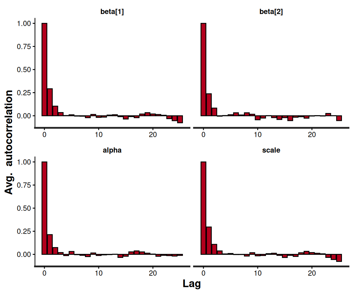
In addition, as mentioned above, we can use rstan built-in functions to visualise and assess convergence, for example as in the following code and the resulting output in Figure 8.4.
# Generates traceplots for the Weibull model's parameters
rstan::traceplot(m$models[[1]])

# Generates autocorrelation plots for the Weibull model's parameters
rstan::stan_ac(m$models[[1]])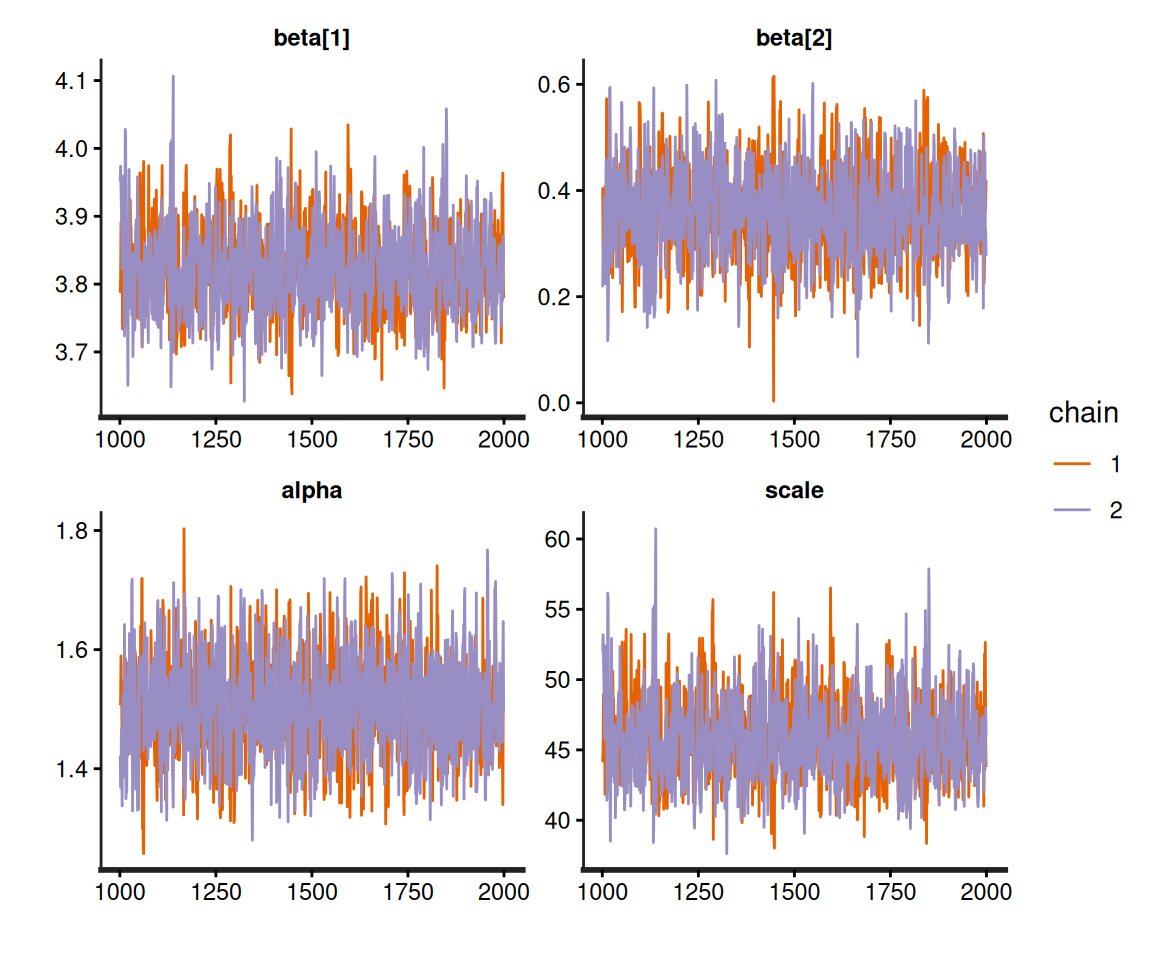
Stan object.
Stan object.
This sort of diagnostic checks should always be performed when running Bayesian modelling, but, again, there is no overheads in carrying them out following a survHE run, because the resulting object is, fundamentally, a rstan output and thus all “standard” Bayesian procedures for post-processing directly apply.
8.4.3 Visualisation and assessment of the survival curves
Once a model has been fitted to observed data and the estimates for the model parameters obtained (e.g. in terms of simulations from the joint posterior distribution, in a Bayesian context), we need to move our analysis to a slightly different level, in which we try and get a sense of the treatment effect, in terms of improvement in survival.
As mentioned in Section 8.3, the main reason why we focus on parametric modelling is because we can use the posterior for the model parameters \(\boldsymbol\theta\) to induce a posterior on the survival curve \(S(t\mid\boldsymbol\theta)=g(\boldsymbol\theta)\), where the function \(g(\cdot)\) depends on the specific model chosen, as shown in Table 8.4.
Especially as the general guideline is to try a number of parametric models to then produce the “base-case” evaluation using the one that “fits the data best” (we clarify the actual meaning of this phrase in the next few sections), it is vital to visualise the results and be able to argue for a specific choice of model, on a combination of numerical and clinical evidence.
Example 8.5. NICE TA174 (continued): estimating the survival curves. survHE has a built-in plot() method, which is based on ggplot2 and can be used to visualise the resulting survival curve for the models fitted using the function fit.models(). For instance, in the NICE TA174 example, we can simply use the following code – notice that we take advantage of the ggplot2 processing facilities and overwrite survHE colouring scheme to ensure that the three models are most distinguishable both when visualised in colour and in grey-scale. We do this by adding the ggplot2 function scale_color_manual() and specifying colours with significant differences in luminance, which are then markedly separated in grey-scale.
# Plots the survival curves for all models and adds some customisation
plot(
  m,
  # Adds the KM estimates (optional)
  add.km=TRUE,
  # Customises the treatment labels (optional)
  lab.profile=c("RFC","FC")
) +
# Customises the position of the legend (optional)
theme(
  legend.position.inside=c(.2,.2)
) + scale_color_manual(values=c("#000000","#1F77B4","#FF7F0E"))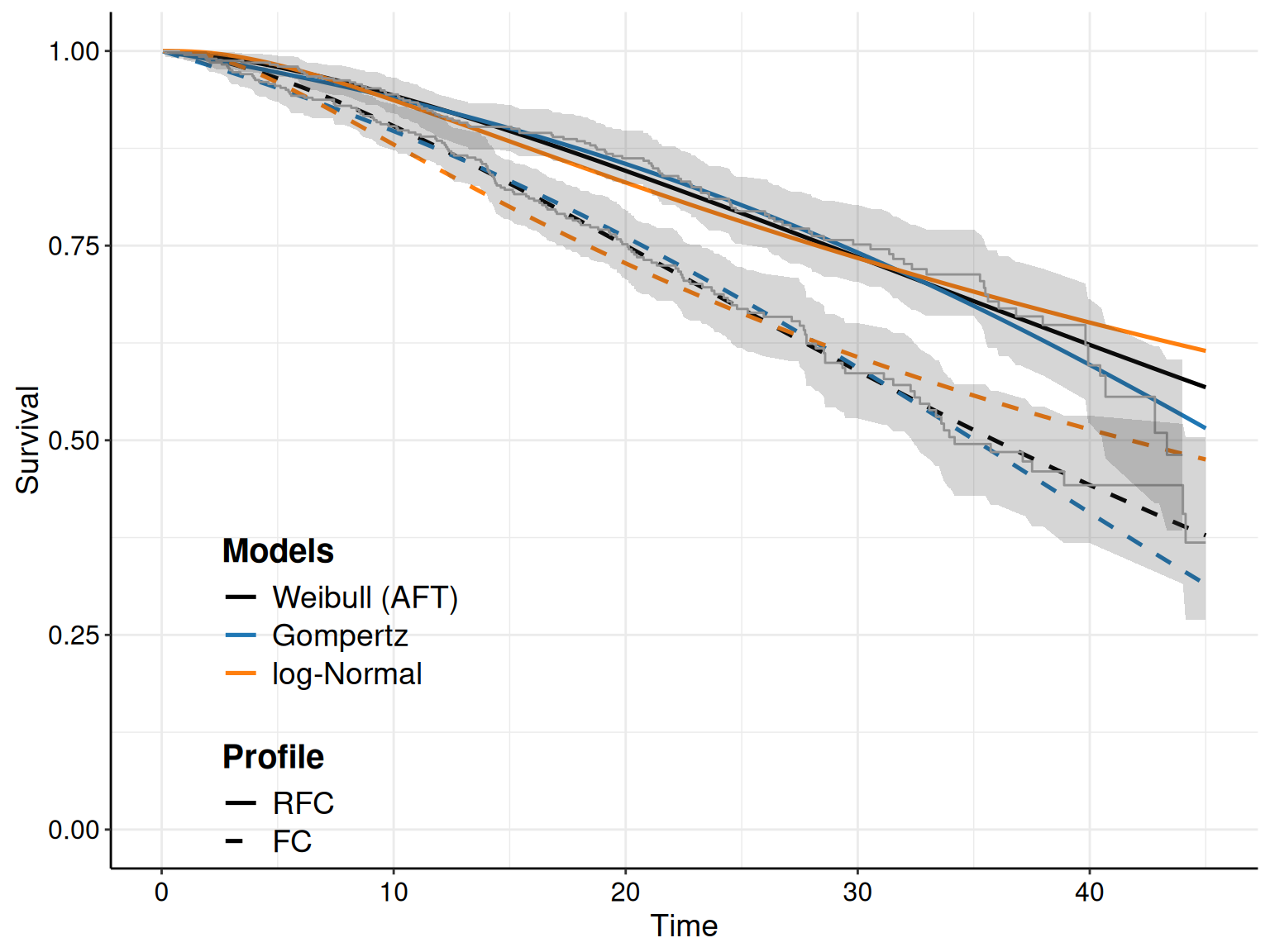
Figure 8.5 shows the KM curves for the two treatment arms with the survival curves estimated from the models in Equations 8.10 – 8.12. Typically, we seek the model that tends to approximate the trajectory in the KM best: for instance, in Figure 8.5 the log-Normal model seems relatively badly calibrated, particularly in the FC arm, where it under-estimates the survival pattern, especially at the beginning of the observation (when the curve is outside the interval around the KM estimates). It also seem to slightly over-estimate survival towards the end of the trial, although in this case the curve is within the KM interval.
As for the other models, the Gompertz does reasonably well for the RFC arm, seemingly capturing the dip in survival at the end of the follow-up. In the FC arm, it perhaps tends to under-estimate survival at the end of the follow-up, perhaps due to some sort of “plateau”, probably due to censoring.
The Weibull model seems perhaps to adapt best to the FC arm, especially at the end of the follow-up, but it is maybe a bit over-optimistic in the last part of the observed data, for the RFC arm.
While perhaps the main objective of the survival analysis in HTA is to produce an estimate of the survival curves, it is generally very helpful to also look at the resulting hazards, to get a sense of the clinical plausibility of the results.
The hazard functions tell us about the instantaneous (and cumulative) risk of experience the event – for instance, it is possible that the risk of dying is very high immediately after a given surgery, but then stabilises or even decreases, over time. Or: it may be completely unrealistic that, with time passing, the risk of a given clinical event becomes lower. These considerations should be used to assess the meaningfulness of alternative model specifications.
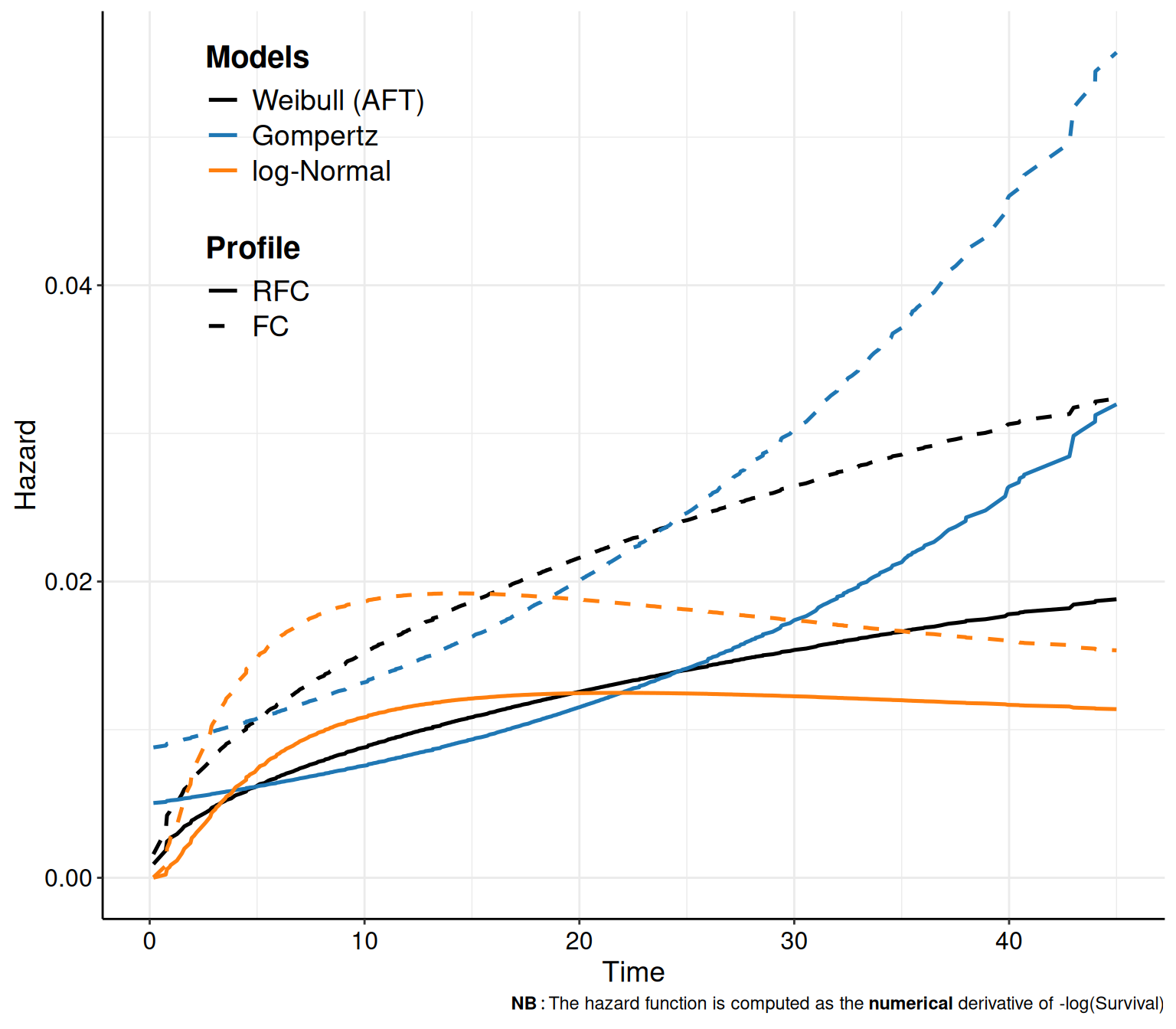
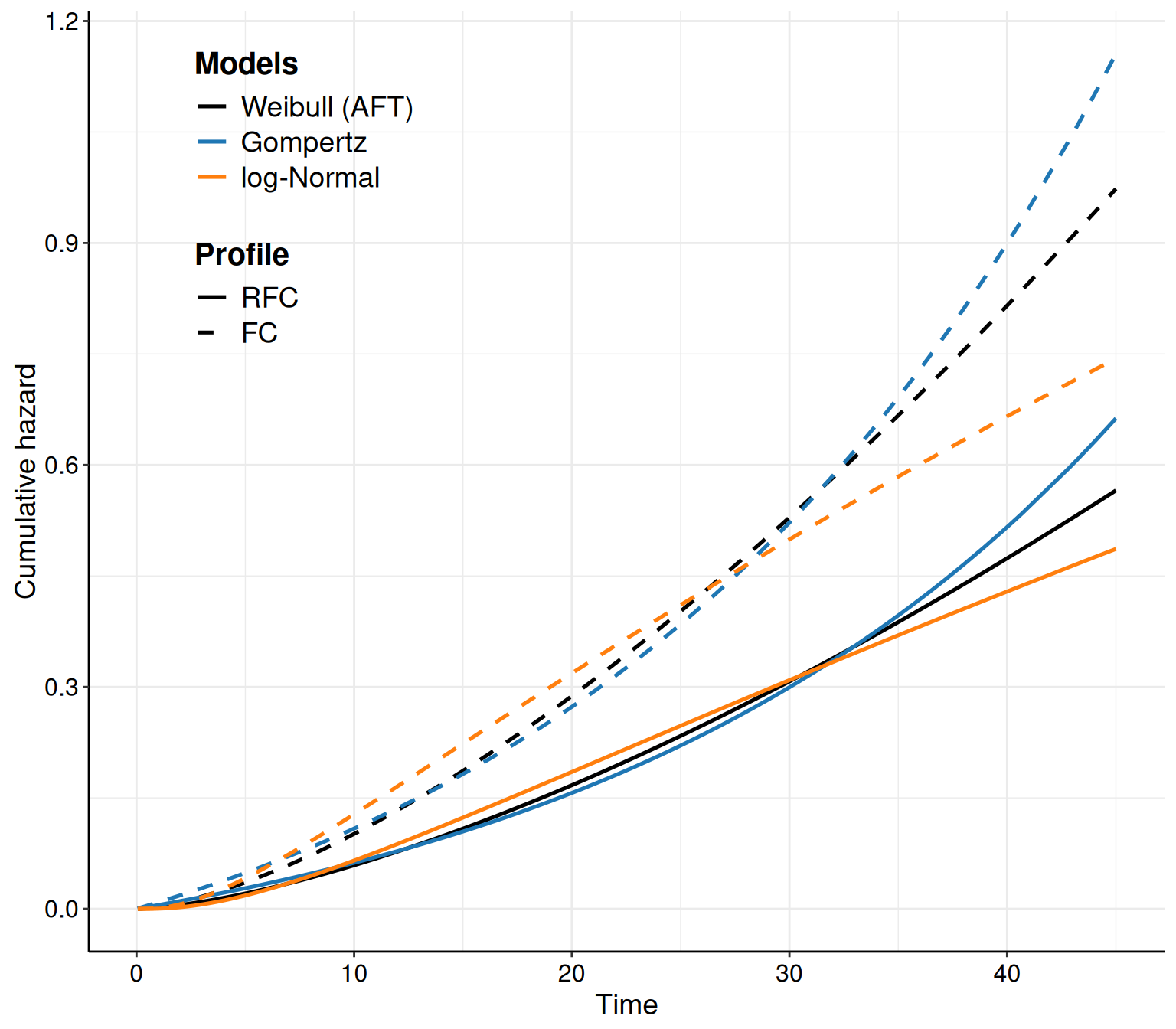
In survHE, we can also plot the hazard and cumulative hazard functions adding the option what="hazard" or what="cumhazard" to the call to the plot() method. The latter (Figure 8.6 (b)) is simply computed using Equation 8.6. The former (Figure 8.6 (a)) is computed as the numerical derivative of \(-\log S(t\mid\boldsymbol\theta)\).
Example 8.6. NICE TA174 (continued): estimating the hazard curves. Figure 8.6 shows the hazard functions derived from the models in Equations 8.10 – 8.12. In Figure 8.6 (a) it is possible to see how the hazard function has a big increase towards the end of the observation period, while it actually decreases for the log-Normal model. While these are related to the mathematical functions describing these two distributions, it is also helpful to compare the trajectories with clinical knowledge about the underlying disease.
Very often, studies based on survival analysis in HTA tend to report graphs such as that in Figure 8.5; these are arguably very important and useful and should be used as the basis for comparison and assessment of model fit and plausibility. However, as they are the output of a statistical modelling, we know that they are subject to inherent uncertainty, because the underlying model parameters are. Thus, it is also important to report a measure of implied uncertainty on the average survival curves.
This is naturally embedded in survHE, which simply needs to add the option nsim to the call for the plot() method. This instructs R to not just take into account the point estimates and plug the relevant values to compute the survival curves; rather, in a full Bayesian approach (particularly when using HMC), we can use the simulations from the joint posterior distribution of all the model parameters \(\boldsymbol\theta\) and propagate the uncertainty to the implied distribution of the survival curve \(S(t\mid\boldsymbol\theta)\).
If the input nsim is set to a value greater than 1, then survHE will automatically construct simulations for the entire distribution of the underlying survival curves. Technically, this automatically calls in the background another survHE function, make.surv(), which produces the required number of simulations.
NoteThe importance of being Bayesian (in survival modelling in HTA) – again
While, strictly speaking, assessing fully the uncertainty in model outputs is not a Bayesian feature only, arguably, the Bayesian philosophy and machinery make this perhaps their key aspect – as discussed in Chapters 1, 2 and 4, the main object of the inference, within a Bayesian approach, is directly the joint posterior distribution, which we can summarise using point estimates, but that, fundamentally, we want to assess and evaluate in its entirety.
As mentioned in Section 5.2.1, this is particularly relevant when there is potential correlation among the model parameters, which we need to reflect appropriately in reporting inference for any function thereof, as is the case in the survival analysis, when we are not just interest in \(\boldsymbol\theta\), as much as we are in \(g(\boldsymbol\theta)=S(t\mid\boldsymbol\theta)\).
Frequentist procedures (such as those used by flexsurv in the background) achieve this through bootstrapping, which, numerically, can be thought of as a (sometimes, but not universally) precise approximation to the full posterior distribution – but again, as the model complexity increases to mimic more closely the complex reality we are trying to understand and estimate, the computational complexity in moving to the Bayesian approach becomes marginally lower and thus potentially much more efficient.
Example 8.7. NICE TA174 (continued): probabilistic sensitivity analysis. The code plot(m,nsim=1000) is sufficient to extend the plot shown in Figure 8.5 and add a 95% interval band around the point estimate for \(S(t\mid\boldsymbol\theta)\).
Looking at multiple survival curves, with the uncertainty around them, within the same plot becomes however quite confusing; for this reason, we can also use the optional argument mods, which allows us to select only one of a few of the distributions fitted in the object m.
For instance, as we have specified in the call to the function fit.models() the option distr=c("wei","gom","lno") to fit the three distributions in the same object, we can simply use the plot() method with the option mods=2 to instruct R to only show the survival curve for the second model (i.e. the Gompertz), as shown in Figure 8.7.
The R code below takes advantage of the fact that the plot() function in survHE generates a ggplot object and, as such, we can manipulate it for further customisation. First, we save the plot onto an object p – this makes it easier to modify its components. Here we choose to add both the KM estimates (with the interval around the step curve), as well as the point and interval estimates for the survival curve for the Gompertz model.
# Saves the plot to a 'ggplot' object, named p, for further customisation
p=plot(
  m,
  # Selects only the Gompertz model (the 2nd in the argument 'distr' when
  # calling the function fit.models() to obtain the object 'm')
  mods=2,
  # Adds the KM curves
  add.km=TRUE,
  # Customises the treatment labels
  lab.profile=c("RFC","FC"),
  # Uses 'nsim=1000' simulations from the posterior to do the PSA
  nsim=1000
)
If we just show the resulting plot (by just calling p in the R terminal), we see that the picture is very busy, with multiple uncertainty bands overlaid on top of each other, which makes it very confusing and hard to process. We can still post-process this object to remove the bands around the KM estimate, while including the step function so that we can assess how closely the point and interval around the survival curve matches the KM.
In fact, the newly created object p contains several elements, including one named layers, which describes the features of the various parts that make up the plot. We can visualise what these are using the command p$layers – in this case, there are four parts. A little trial and error (or deeper knowledge of the ggplot machinery…), allows us to identify that the fourth one:
p$layers[[4]]mapping: x = ~time, y = ~S, ymin = ~lower, ymax = ~upper, group =
~as.factor(strata:object_name)
geom_ribbon: na.rm = FALSE, orientation = NA, lineend = butt, linejoin = round,
linemitre = 10, outline.type = both
stat_identity: na.rm = FALSE position_identityis actually the one we want to remove, i.e. the interval bands around the KM estimates. We can do this by setting that layer to NULL and then show the revised object p.
# Removes the 'ggplot' layer showing the interval estimate around the KM curves
p$layers[[4]]=NULL

# Shows the revised plot and customise the position of the legend
p + theme(legend.position.inside=c(.2,.6))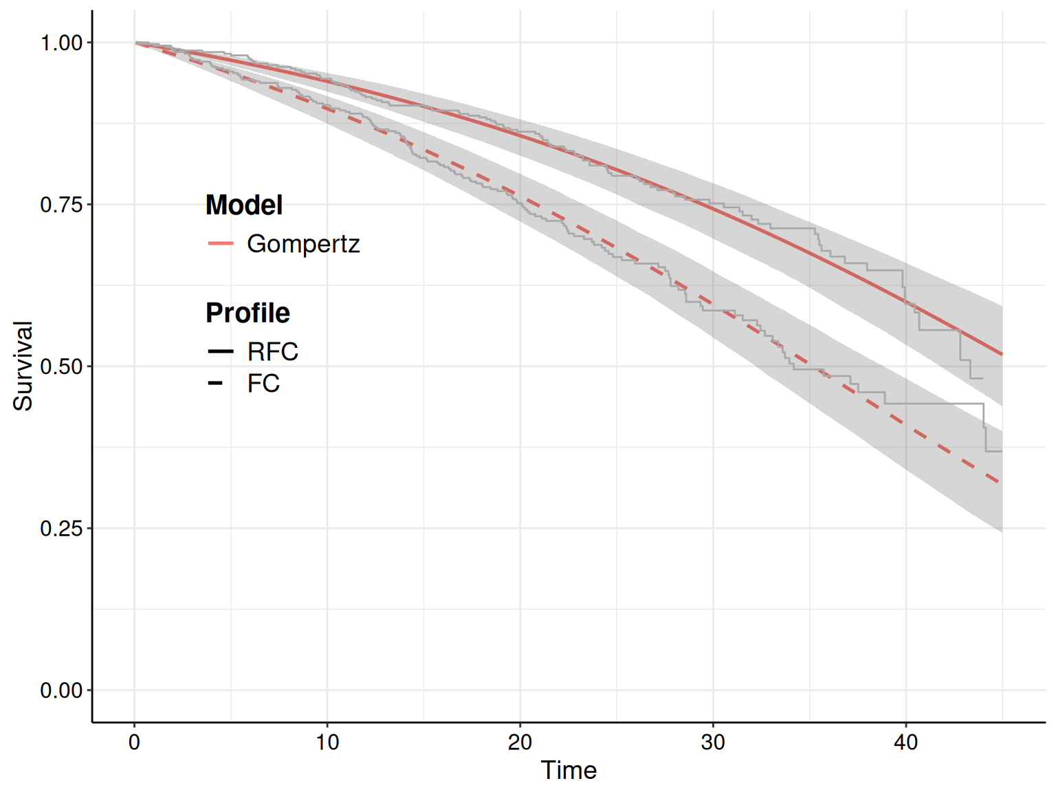
The resulting graph in Figure 8.7 becomes much more readable and helpful – with a clear measure of how well the Gompertz survival curve matches the observed data. For the most part, the KM estimates are all enclosed within the interval band around the point estimate for \(S(t\mid\boldsymbol\theta)\) – with the only exception of the FC arm, at the very end of the observation period. Throughout most of the follow-up, the solid curves do a reasonable job at approximating the trajectory shown in the observed data – this is one of the key feature we seek when visualising the estimated survival curves.
8.4.4 Model selection
As we have hinted at earlier, given that the advice is to try several distributional assumptions on a given dataset, it obviously becomes important to be able to select one of the options as “the best” – of course, what this qualifier actually means, remains a bit vague. We know that whatever our choice, we will most likely not be in a position of characterising perfectly to true underlying data-generating process.
In line with the discussion of Section 5.3 and Section 6.2.6, it is helpful to consider some model-fitting criteria (e.g. DIC, in a Bayesian context), to say something on “how well does a single model fit the observed data” – we return to this idea in Section 8.4.6.
Example 8.8. NICE TA174 (continued): model selection. Figure 8.8 illustrates how we can use survHE to visualise and compare the model fitting performance for the competing models. Figure 8.8 (a) uses the function model.fit.plot() with the only argument type="DIC" to display a bar-chart with the absolute value of the DIC for the three models.
# Model fitting plot (specifies the DIC)
model.fit.plot(m,type="DIC")

# Model fitting plot (on a relative scale, wrt the best fitting model)
model.fit.plot(m,type="DIC",scale="relative")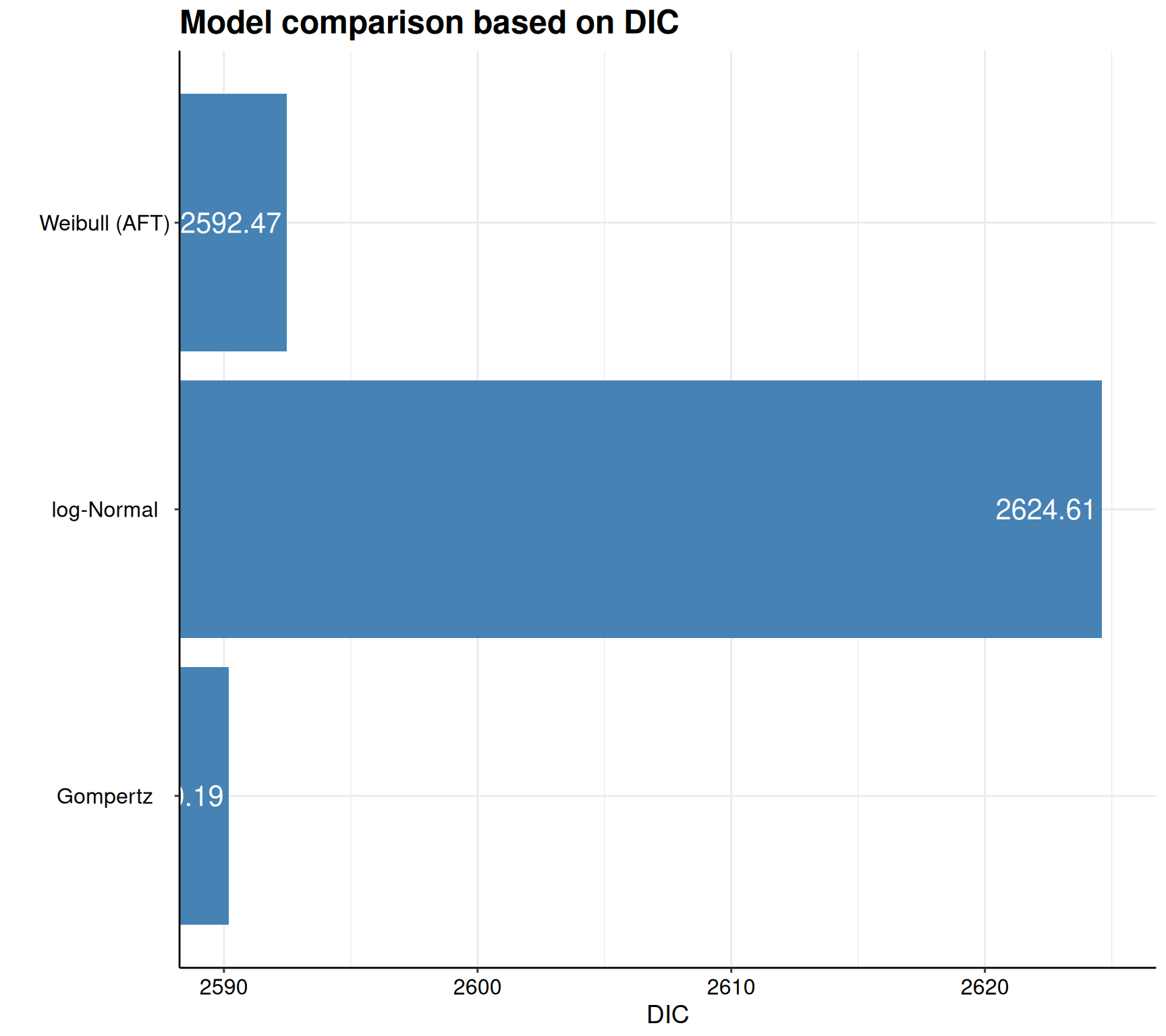
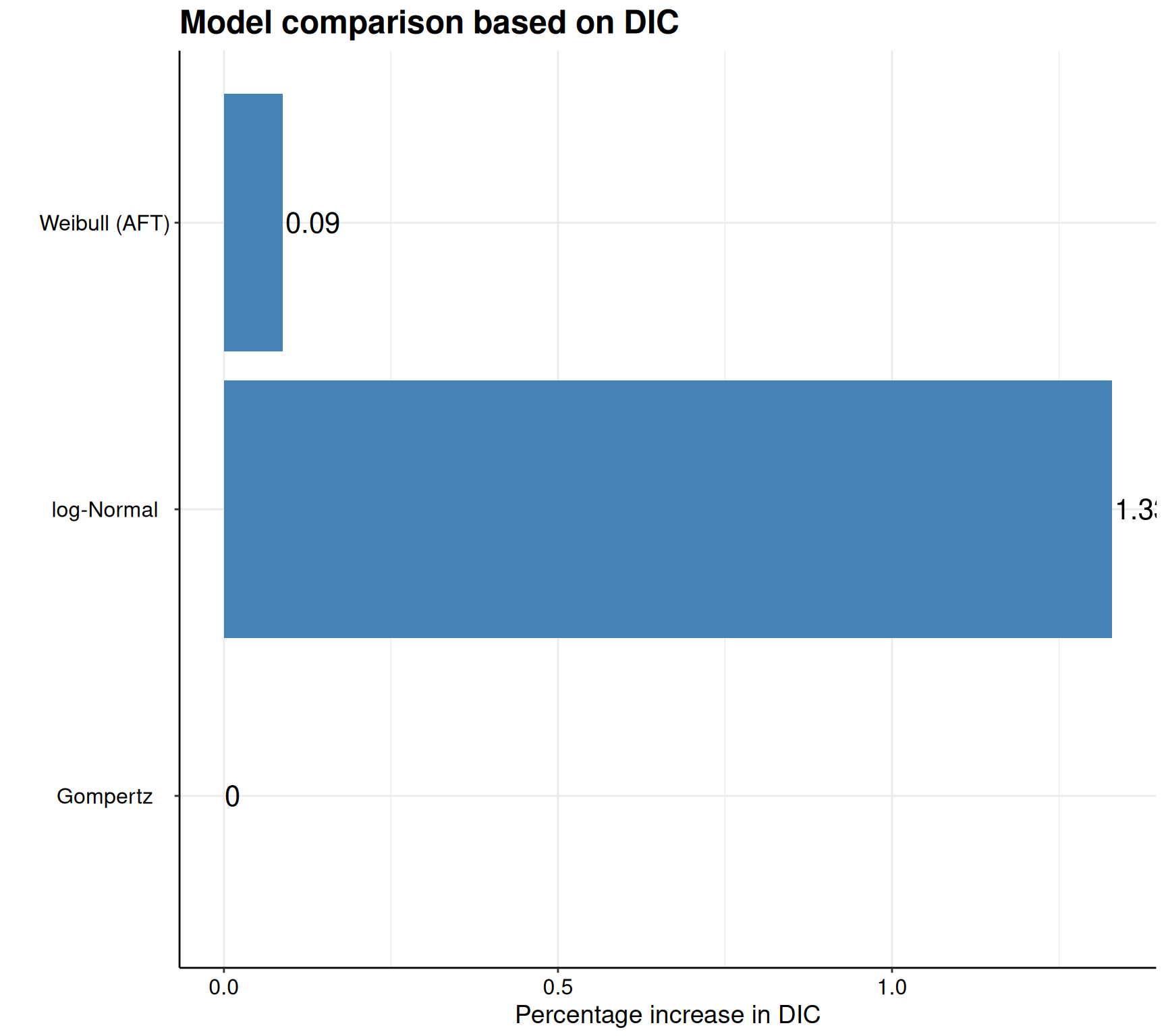
The graph seems to indicate that there is little difference, in the model fit, between the Weibull and the Gompertz model, but that the log-Normal is substantially worse, based on the DIC.
Figure 8.8 (b) also adds the optional argument scale="relative" to display the bar-chart using the best-fitting model as reference and showing the percentage incremental in the DIC from the other two. Again, this highlights that the log-Normal does have a relatively higher value for the DIC, while the Weibull only contributes an increase in DIC (i.e. worse performance) of 0.1%. Displaying the results on a relative scale is sometimes useful to appreciate the magnitude of how much better one of the model seems to be doing, in comparison to the others.
8.4.5 Separate modelling by treatment arm
While Example 8.8 indicates that the Gompertz model may be the best fitting, albeit marginally over the Weibull, the analysis of Example 8.5 seems to indicate that, actually, there may not be a single model fitting the observed data best, in both the treatment arms. This is not uncommon, particularly when we are not able to account for more potential covariates of interest and can only control for the treatment arm.
In these situations, we may stipulate that instead of modelling the linear predictors as functions of the treatment indicator, as we have specified in Equations 8.10 – 8.12, we could run separate models by subsetting the data to only include the controls and then the intervention arm, with only an intercept in the expressions for \(\eta_i\). This approach effectively assumes that both the location and the ancillary parameters depend on the treatment arm (as they are estimated using separate models).
Generally speaking, HTA submissions tend to focus on a main model (as the base-case analysis) and Latimer (2011) comments that:
Fitting separate parametric models to each treatment arm involves fewer assumptions, although it does also require the estimation of more parameters. While fitting separate parametric models to individual treatment arms may be justified, it is important to note that fitting different types of parametric model (for example a Weibull for one treatment arm and a log normal for the other) to different treatment arms would require substantial justification, as different models allow very different shaped distribution.
Example 8.9. NICE TA174 (continued): separate modelling by treatment arm. We can use the following code to run the models on the two subsets of the TA174 data, filtering for the treatment arm and thus selecting only the controls or only the intervention arm. In the formula to describe the linear predictor, we only specify the intercept term using the R notation ~1.
# Model for the control arm only
m.ctl=fit.models(
  Surv(time,status)~1,
  data=data |> dplyr::filter(treatment=="FC"),
  distr=c("wei","gom","lno"),method="hmc"
)

# Model for the treatment arm only
m.trt=fit.models(
  Surv(time,status)~1,
  data=data |> dplyr::filter(treatment=="RFC"),
  distr=c("wei","gom","lno"),method="hmc"
)
The resulting model fit can be summarised again using the model.fit.plot() function: the option stacked=TRUE instructs R to create grouped bar-charts so that it is easier to compare across different objects (m.ctl vs m.trt, here).
# Then assess model fit across the models
model.fit.plot(FC=m.ctl,RFC=m.trt,type="DIC",stacked=TRUE)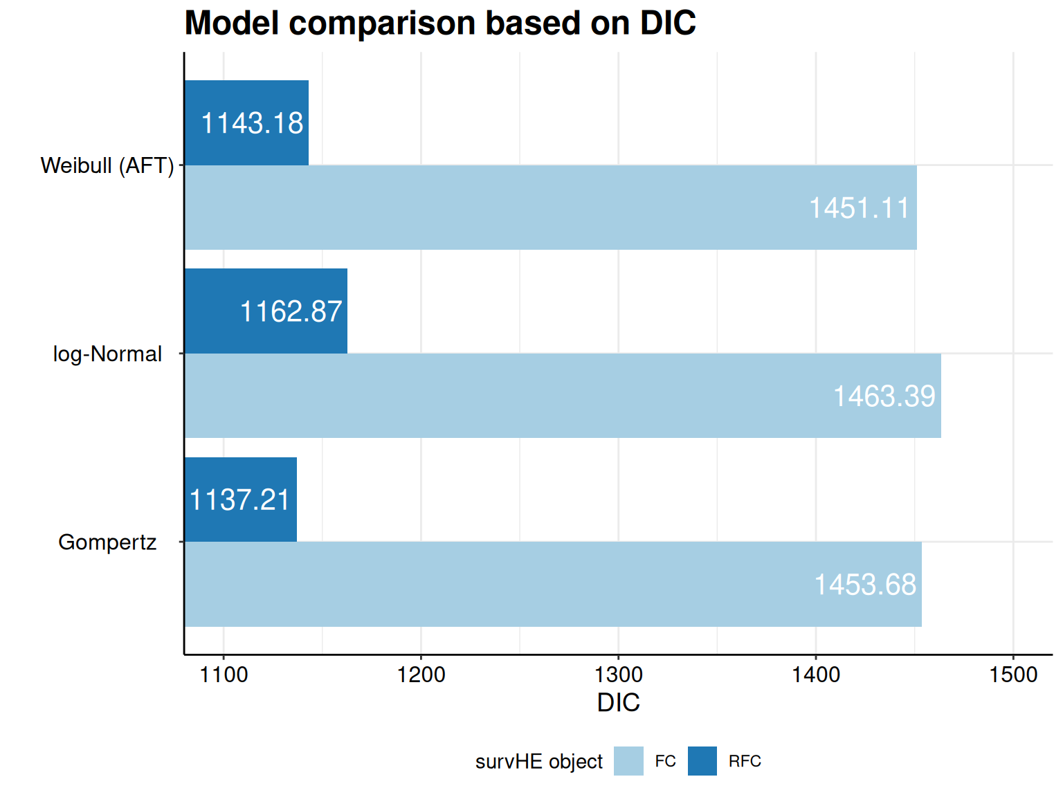
As is possible to see, this confirms the fact that the Gompertz does (marginally) better than the Weibull for the controls (FC), but the reverse is true for the treatment arm (RFC).
8.4.6 Extrapolation
As mentioned in Section 8.3, in “standard” biostatistical analysis of time-to-event data, the main objective is to estimate the effect of a set of covariates (including, most importantly the treatment arm) on the survival time, as well as an estimate of the median survival – this is because most often, trial data at least cover the situation in which at least half of the sample experience the event of interest.
In HTA, the main focus is not so much on either of these objectives, but rather in determining the long-term benefits of a given treatment (see Figure 8.2). We then face a complicated assessment process, which by necessity needs to mix statistical and clinical considerations, together with unavoidable uncertainty about the extrapolation into the future.
On the one hand, we want to ensure that the model we select is able to represent the observed data (within the trial follow-up) as well as possible – as in the discussion on model fitting in Example 8.8. This is perhaps the more “statistical” side of the assessment.
On the other hand, we also want to select a model that has clinical plausibility in the long-term extrapolation, i.e. for which the resulting survival at a time reasonably far in the future is generally justifiable and defensible, given the clinical expertise. Interestingly, because extrapolation, by nature, has to do with data that have not yet occurred, there is very little that we can do to assess how reasonable it is, simply based on model fitting statistics.
Consequently, model fitting cannot be an overarching guiding principle to selecting one of the models, because it can only tell us about how well a given distributional assumptions setup does with respect to the observed data – but can say nothing at all about the extrapolation period. Mathematically, this is evident if we consider model fitting criteria based on the deviance, which in turn is a function of the (log)likelihood, i.e. given observed data (and a situation not too dissimilar to the one discussed in Chapter 10).
One important implication of this discussion is that it is crucial to visualise the extrapolated curves and, even more importantly, to accept the inherent and unavoidable uncertainty that is associated with this process.
Example 8.10. NICE TA174 (continued): extrapolation. Figure 8.10 shows the extrapolated curves for the models in Equations 8.10 – 8.12, over a time horizon spanning up to \(t=180\) months (i.e. 15 years).
It is possible to directly add this to the plot() function in survHE by simply adding the optional argument t. In this case, we can use code such as t=seq(0,180), to extrapolate the underlying survival curves up to \(t=180\), as required.
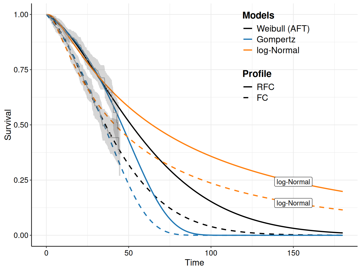
As is possible to see, although it does have a decent fit to the observed time period (e.g. around 45 months), the log-Normal model does extrapolate in a rather peculiar way, with curves that, even at \(t=180\) would suggest a rather high probability of not having experienced the event (progression) – the two curves labelled as “log-Normal” are well above 10%, for both treatment arms. This may be considered as unrealistic, drawing on clinical experience and thus the log-Normal model would be considered as unrealistic and discarded on that basis.
Irrespective of the model fitting statistics, we can continue to consider the clinical plausibility of all the models, from the visualisation of the extrapolated survival curves: if we consider the Gompertz and the Weibull, we may stipulate that the latter tends to give a survival probability that is just too high, at later points in the time horizon. For instance, in the RFC arm, \(S(t\mid\boldsymbol\theta)>0.12\), at around 100 months, which clinicians may deem too optimistic. Similar considerations may apply, perhaps to a lower extent, for the FC arm too where \(S(t\mid\boldsymbol\theta)\approx 0.04\), at \(t=100\).
On the other hand, the Gompertz model may penalise particularly the FC arm, by dropping the survival curve a bit too abruptly, although the point in the time horizon at which the survival curves for the two arms hit 0 may be deemed reasonable by clinical experts.
In line with the discussion in Section 8.4.5, we may also decide to consider different distributional assumptions for the two treatment arms – we can isolate the Weibull survival for FC and the Gompertz survival for RFC using the following code (this is effectively identical to removing all the other curves from Figure 8.10).
plot(
  # Selects and names the 'survHE' objects to plot; automatically creates a
  # list combining 'm.ctl' and 'm.trt' (so 3+3=6 models overall)
  FC=m.ctl,RFC=m.trt,
  # Selects which of the models in two objects to plot:
  #  mods=1 => 1st model in m.ctl => Weibull model for FC
  #  mods=5 => 2nd model in m.int, 5th overall => Gompertz for RFG
  mods=c(1,5),
  # Adds KM and extrapolates to 180 months
  add.km=T, t=seq(0,180)
) + scale_color_manual(values=c("#000000","#1F77B4"))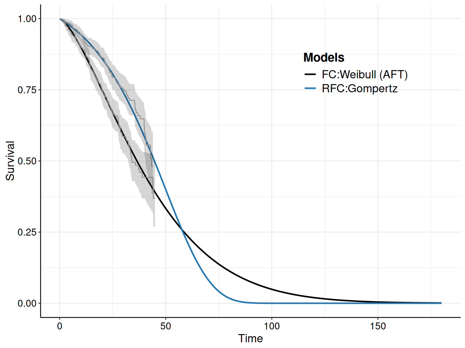
Figure 8.11 highlights that, for this particular analysis, we would be willing to violate the assumption of proportional hazard, as the curves cross just after \(t=50\).
The analysis in Example 8.10 highlights the inherent uncertainty in the extrapolation process – the data seem to suggest that in the control arm the Weibull distribution is a very good fit and, perhaps, the extrapolated curve is meaningful clinically. The trajectory of the Gompertz in the intervention arm, as well as the violation of PH, may be real, as dictated by a fast waining treatment effect, or maybe is artificially influenced by small numbers at the end of the trial follow-up when we see a marked number of events, which in turn, perhaps unduly, pulls the extrapolated survival curve towards 0, very quickly.
Note 8.5: Hazardous ratios
The subtle nature of the PH assumption and the use of HRs as a main measure of inference are a well known issue in the biostatistical (and causal inference) literature. Notably, Hernán (2010) highlights that hazard ratios compare the hazard rates between treatment groups at specific time points, conditional on survival up to that time. This implies that the HR reflects the instantaneous risk among individuals who have survived to a particular time, rather than providing an overall measure of treatment effect across the entire study population.
In addition, HRs are non-collapsible (see also Example 11.1 in Section 11.2), meaning that HRs calculated for the entire study population may differ from those estimated within subgroups, even in the absence of confounding. This property can lead to discrepancies between marginal and conditional estimates, complicating the interpretation of HRs as measures of average treatment effect. This is also related to the fact that, as time progresses in a study, the way in which individuals remain at risk can change non-uniformly in different treatment arms. This dynamic can introduce selection bias, as the groups being compared may no longer be comparable due to differential survival, potentially distorting the HR.
This latter feature has the potential of fundamentally generating a violation of the PH assumption; crossing of the underlying survival curves may be generated by a “real” non-PH in the underlying DGP, but may also result as a consequence of selection bias, especially in the presence of large censoring.
Ultimately, it is very possible that with relatively immature data (which are often a feature of HTA modelling based on survival), a single dataset is just not good enough to provide, at the same time, the best characterisation of the observed trial data, as well as a clinically meaningful extrapolation to the long-term effects.
8.5 Advanced survival modelling in HTA
Recent research developments in statistical modelling for survival data in HTA have concentrated on flexible alternative to the “standard” parametric models described above. For example, drawing on methodology originally introduced by Royston and Altman (1994), Jansen (2011) and Jansen et al. (2015) have presented methods based on “fractional polynomials”. These are flexible functions used to model time-dependent effects by allowing non-linear transformations of time using non-integer powers. One drawback of this method is that they can be quite computationally intensive and hard to interpret, because of the nature of the fundamental parameters.
Another interesting approach to provide more flexibility in the modelling of censored time-to-event data is to use “poly-hazard” models. The main idea is to describe survival as arising from multiple independent failure processes, each with its own hazard function – essentially, this amounts to assuming a mixture of a number of terms, each characterised by an independent hazard function. One convenient model is to assume a poly-Weibull structure (Demiris et al., 2015; Benaglia et al., 2015), where a set number of individual Weibull hazard functions combine additively to capture complex, multi-risk survival patterns.
Hardcastle et al. (2025) have recently produced computational advancements to expand on the basic poly-hazard model and allow model- and variable-selections within the MCMC algorithm. In particular, the model allows data-driven selection of the number of components, can switch covariates on and off (by allowing their coefficient to spike at 0) and jump across different distributional assumptions for the hazards.
More recently, much of the research has focused on using splines, which are flexible, piecewise polynomial functions that model complex, non-linear relationships over time by smoothly connecting intervals at predefined knots. While, especially in a Bayesian context, fitting splines can still pose computational challenges, their interpretation and use for extrapolation is much simpler and thus they are currently one of the “good” methods to use in the context of survival analysis in HTA.
8.5.1 M-splines models
M-splines (Ramsay, 1988) are a set of non-negative, piecewise polynomial functions that provide a flexible yet smooth representation of hazard over time, defined over a series of “knots”, which are specific time points that partition the time axis. By default, the knot locations are automatically selected based on quantiles of the observed event times, but it is possible to select specific values, depending on the data at hand.
A relevant application in HTA is the model specified by Jackson (2023) and defined as \[ h(t\mid\boldsymbol\theta) = \phi\sum_{k=1}^K \omega_k b_k(t), \tag{8.13}\] where \(\phi>0\) is the baseline hazard scale parameter, \(\boldsymbol\omega=(\omega_1,\ldots,\omega_K)\) is a vector of coefficients for the M-spline basis terms and \(b_k(t)\) are deterministic functions of time \(t\), known as “basis functions”.
The hazard function is expressed as a linear combination of the basis functions, with coefficients estimated within a Bayesian framework. Beyond the boundary knots, i.e. outside the range of the data, the model assumes that the hazard remains constant, adopting the value at the last knot. This assumption provides a pragmatic approach to extrapolation, acknowledging uncertainty in areas lacking data while avoiding unwarranted complexity.
In general, the baseline hazard scale parameter is modelled by defining a prior on the log scale: \(\log\phi \sim \text{Normal}(0,\text{sd}=20)\), although it is possible to include dependence of the hazard function on a set of \(C\) covariates \(\boldsymbol{x}=(\boldsymbol{x}_1,\ldots,\boldsymbol{x}_C)\) by assuming a PH model in which \(\phi^*(\boldsymbol{x})=\phi\exp(\boldsymbol\beta^\top \boldsymbol{x})\), with a default prior \(\beta_1,\ldots,\beta_C \stackrel{iid}{\sim}\text{Normal}(0,\text{sd}=2.5)\).
The M-spline coefficients are subject to the constraint that \(\sum_{k=1}^K \omega_k =1\) and are modelled using partial pooling to ensure smoothing, with the following specification \[ \gamma_k=\log\left(\frac{\omega_k}{\omega_1}\right)\sim\text{Logistic}(\mu_k,\sigma), \] where \(\gamma_1=\mu_1=0\) and, in general \[ y\mid \mu,\sigma \sim \text{Logistic}(\mu,\sigma) \quad\Rightarrow\quad p(y\mid\mu,\sigma)=\frac{1}{\sigma}\exp\left(-\frac{y-\mu}{\sigma}\right)\left(1+\exp\left(-\frac{y-\mu}{\sigma}\right)\right)^{-2}. \] This formulation is useful to prevent overfitting, effectively penalising excessive flexibility and allowing the model to adapt its complexity based on the amount and quality of the available data.
The location parameters \(\boldsymbol{\mu}=(0,\mu_2,\ldots,\mu_K)\) are selected using a data-driven procedure based on the location of consecutive knots for the basis functions, so as to ensure that, in the prior, for each \(\mu_k\), the corresponding weight \(\omega_k\) implies a constant hazard.
The scale parameter \(\sigma\) controls the level of smoothness of the fitted hazard curve and it is given a default prior \(\sigma\sim \text{Gamma}(2,1)\) – this amounts to considering \(\Pr(\sigma>4)\approx 0.1\). If \(\sigma\rightarrow 0\), then the hazard is closer to constant.
Another way to include dependence on the covariates \(\boldsymbol{x}\) while also relaxing the PH assumption is to add a term to the location of the Logistic distribution, so that it becomes \(\mu+\boldsymbol{\delta}_k^\top \boldsymbol{x}\), where \(\boldsymbol\delta_k=(\delta_{k1},\ldots,\delta_{kC})\) and \(\boldsymbol\delta_1=\boldsymbol{0}_C\). For each covariate \(\boldsymbol{x}_c\), the resulting coefficient \(\delta_{kc}\) quantifies the level of departure from the basic PH assumption. In the prior, \(\delta_{kc}\sim\text{Normal}(0,\tau_k)\), where \(\tau_k\sim \text{Gamma}(2,1)\), by default.
Jackson (2023) provides more discussion on the modelling framework for Bayesian M-splines, while Phillippo et al. (2024) discuss an application of this family of models in the context of multilevel NMA (see Chapter 11) and, in particular, the use of Random Walk priors to induce smoothness.
Example 8.11. NICE TA174 (continued): modelling M-splines using survextrap. Similarly to survHE, the M-splines model is fully implemented in the R package survextrap (Jackson, 2023). Detailed tutorials are also included in the software website https://chjackson.github.io/survextrap/ and in the GitHub repository https://github.com/chjackson/survextrap/. We demonstrate the basic use of survextrap in the following.
The first task is to set up the basic structure of the M-spline model. The fundamental information, which is coded up in the survextrap function mspline_spec(), involves: i) the model formula (which specifies the linear predictor – in this case, we only consider the intercept and model the impact of the covariates later); ii) the dataset to be analysed (which is used to construct the knots, based on the quantiles of the observed data); iii) the number of basis functions (in this case, 6), which determine the “degrees of freedom” of the M-spline procedure; and iv) the additional knots (in this case up to \(t=180\)), which are used to extrapolate beyond the observed time-frame.
# Loads the package
library(survextrap)

# Spline specification
mspline=mspline_spec(
  formula=Surv(time,status)~1,
  data=data,
  # Defines the number of basis function (=degrees of freedom of the spline)
  df=6,
  # Define additional knots (for the extrapolation part)
  add_knots=180
)
The resulting object mspline stores a set of variables that are instrumental to actually fitting the model in Equation 8.13.
The Bayesian estimation is actually performed by the call to the survextrap function survextrap(), specified as in the following code.
# Runs the model
msp=survextrap(
  formula=Surv(time,status)~treatment,
  data=data,
  mspline=mspline,
  chains=2,iter=4000
)
Here, we first specify the model formula, which includes the treatment arm as a covariate. In addition, we pass the set up information stored in the object mspline and then select 2 chains, each with 4000 iterations for the HMC run – more options are available and described both in the package vignettes (https://chjackson.github.io/survextrap/articles/) and the R help. The results can be visualised by simply calling the object msp in the R terminal.
Individual data: 810 individuals, 248 events
External data: 1 period
M-spline survival model
6 knots, degree 3, 7 basis terms.
Fitted using MCMC
Smoothness SD: full Bayes
Priors:
  Baseline log hazard scale: normal(location=0,scale=20)
  Log hazard ratios:
  treatmentRFC: normal(location=0,scale=2.5)
  Smoothness SD: gamma(shape=2,rate=1)
Sample of 4000 from the posterior
Posterior summary:
# A tibble: 11 × 9
   variable basis_num term           median    lower   upper      sd  rhat ess_bulk
   <chr>        <dbl> <chr>           <dbl>    <dbl>   <dbl>   <dbl> <dbl>    <dbl>
 1 alpha           NA <NA>          0.499    0.145    0.800  0.165   1.000    1654.
 2 coefs            1 <NA>          0.00904  0.00390  0.0164 0.00324 1.00     2181.
 3 coefs            2 <NA>          0.0188   0.00994  0.0316 0.00562 1.00     2920.
 4 coefs            3 <NA>          0.0371   0.0204   0.0645 0.0111  1.000    2948.
 5 coefs            4 <NA>          0.0711   0.0459   0.110  0.0164  1.00     2708.
 6 coefs            5 <NA>          0.109    0.0620   0.188  0.0329  1.00     2131.
 7 coefs            6 <NA>          0.688    0.438    0.814  0.100   1.000    1704.
 8 coefs            7 <NA>          0.0658   0.00303  0.220  0.0581  1.00     1699.
 9 loghr           NA treatmentRFC -0.544   -0.800   -0.288  0.129   1.00     2762.
10 hr              NA treatmentRFC  0.580    0.449    0.749  0.0759  1.00     2762.
11 hsd             NA <NA>          1.19     0.533    2.60   0.537   1.00      824.
This returns first detailed information on the prior setup, including the default distributions selected for the model parameters. In the priors block, Baseline log hazard scale is \(\log(\phi)\) in Equation 8.13; treatmentRFC indicates the coefficient \(\beta\) for the only covariate included in the model, in this case; and Smoothness SD indicates \(\sigma\) above.
In the main body of the table, for each model parameter, the summary reports the posterior median, 95% interval estimates and standard deviation, as well as some (rstan-based) convergence metrics. The parameter reported as alpha is the baseline log-hazard scale, i.e. \(\log(\phi)\) in the notation of Equation 8.13. The parameters labelled as coefs indicate the elements of the vector \(\boldsymbol\omega\), i.e. the coefficients for the basis functions. The parameter loghr indicates the coefficient \(\beta\) for the covariate included in the linear predictor (the treatment arm), while hr is its exponentiated value, i.e. the HR. Because the underlying M-spline model assumes PH, this estimate is comparable with that provided by the Gompertz model in Example 8.2. Finally, the parameter indicated as hsd is the smoothing scale \(\sigma\).
The object msp can be further processed using built-in functions from survextrap or other R packages (including rstan or ggplot2). For instance, we can reconstruct the estimates survival curves using the following code. Here, for consistency with survHE, we use the mean (rather than the median) and the 95% interval estimates and save these in the object S.
# Extracts the survival curves
S=survextrap::survival(
  # For consistency with survHE, selects the mean (rather than the median)
  msp,summ_fns=list(mean=mean,~quantile(.x, probs=c(0.025, 0.975)))
)
This, in turn, can be used to plot the survival curves. Figure 8.12 (a) (generated by the code below) shows the fitted curves using survHE and the Weibull and Gompertz models, as well as the M-spline based estimates computed by survextrap. Here we can take full advantage of ggplot2 to combine different objects into the same plot, effectively by customising the survextrap object S to align with the survHE output.
# Puts together the data to show plots from survHE and survextrap
plot(
  # Plots the fit for Weibull and Gompertz models
  m,mods=c(1,2),add.km=T,t=seq(0,180),
  lab.profile=c("RFC","FC")
) +
  # Adds the data from the M-spline survival curves
  # (recodes the treatment to strata, to be consistent with survHE)
  geom_line(
    data=S |> mutate(
      model="M-spline",
      strata=case_when(
        treatment=="FC"~"treatmentRFC=0",TRUE~"treatmentRFC=1"
      ) |> factor(level=c("treatmentRFC=1","treatmentRFC=0"))
    ),
    aes(t,mean,col=model,linetype=strata),size=0.9
    ) +
scale_color_manual(values = c("#000000", "#1F77B4", "#FF7F0E")) 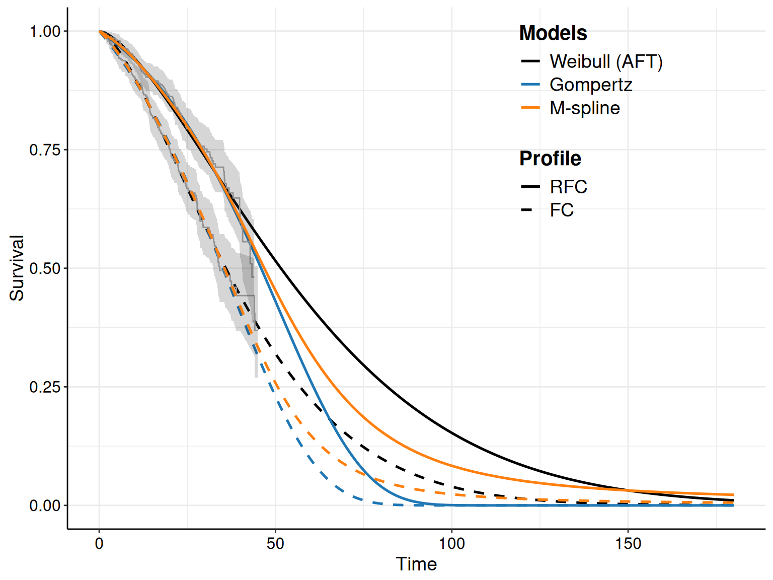
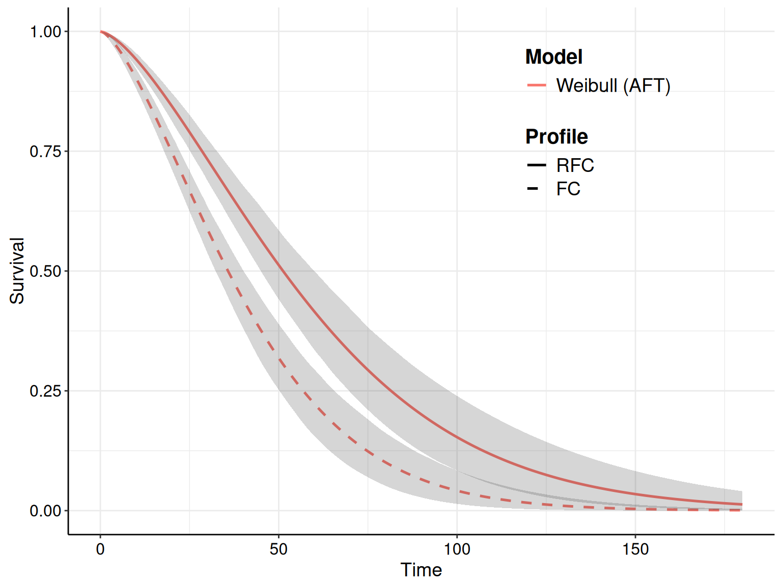
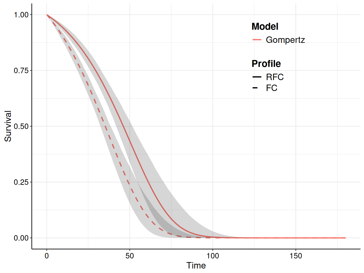
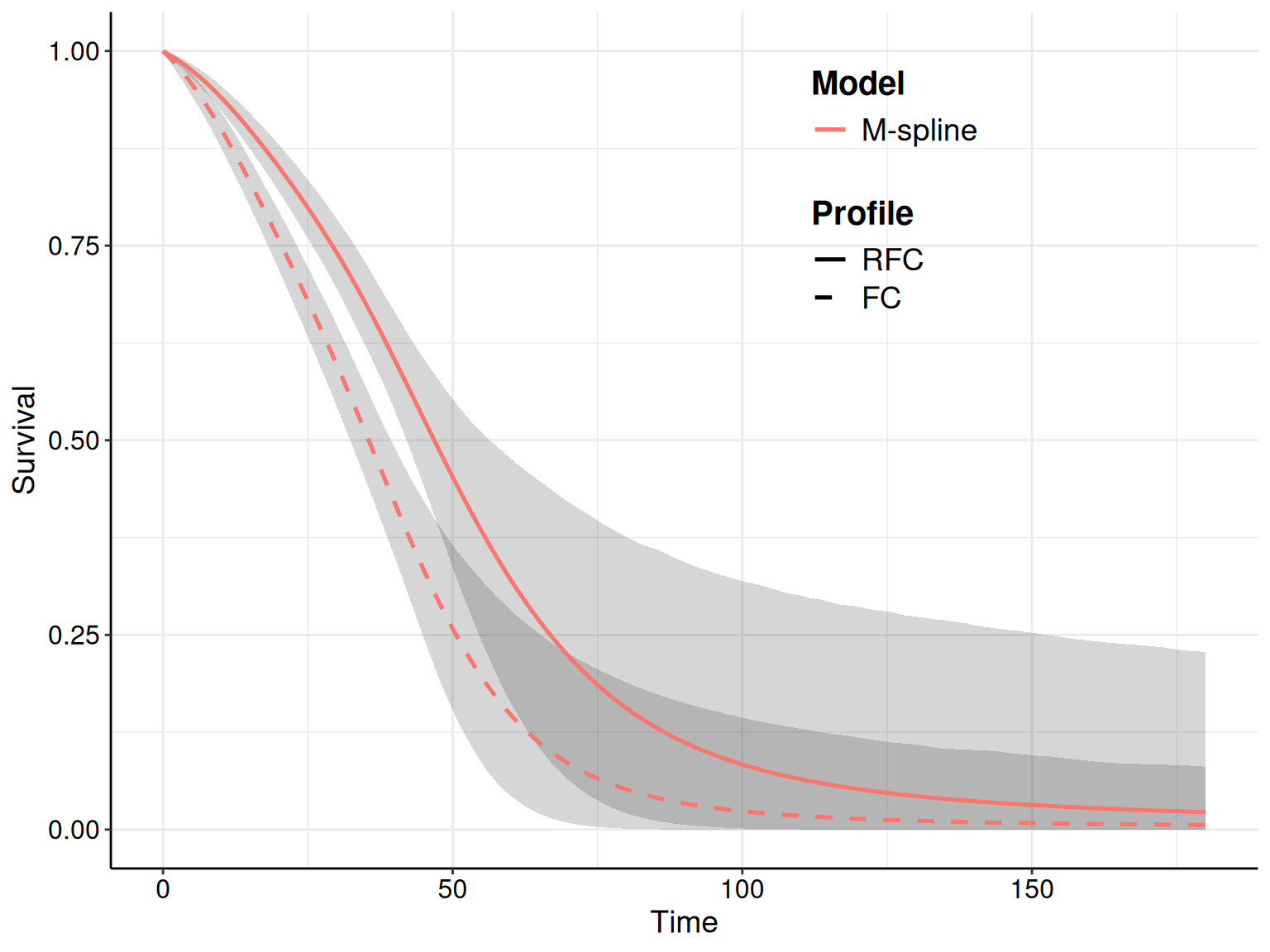
While both the parametric models and the M-spline cover well the observed data, the extrapolations are quite different. The M-spline model seems to produce slightly higher curves towards the end of the extrapolation, in comparison to the Weibull and even more so to the Gompertz models. This latter seems to suggest a steeper decrease towards 0, especially for the treatment arm.
The differences are better appreciated in Figures 8.12 (b)–8.12 (d), which show the survival curves together with a 95% interval estimates for the Weibull, Gompertz and M-spline models, respectively. Interestingly, the M-spline model shows substantial uncertainty in the extrapolation period, in comparison with the parametric models. This is not surprising: there are no observed data beyond the end of the follow-up and thus the M-spline responds by giving very wide interval estimates for the survival curves. Conversely, the two parametric models are “mathematically forced” to give increasingly narrow uncertainty as time progresses along the \(x\)–axis.
In a sense, neither model is necessarily “correct”: on the one hand, the parametric models naturally encode in their mathematical formulation the fact that, eventually, survival will go down to 0 – if we wait for long enough. On the other hand, M-splines respond to the lack of observed data by showing large uncertainty around the survival (basically being more naturally agnostic about “how long is long enough”).
More pragmatically and importantly, this consideration highlights the fact that, in reality, the observed data on a limited follow-up are most often just not informative enough to have a model that fits them as well as possible, while also extrapolating in the most sensible way possible…
8.5.2 Including external information
The Bayesian framework allows naturally the incorporation of different sources of information, which is particularly relevant in the case of survival modelling based on limited/immature data for the follow-up period, but for which we need to extrapolate over a much longer time horizon.
One typical situation is when, alongside the individual-level data for the follow-up, we also have information, perhaps in the form of aggregated or summary data, over the longer term. One common way to deal with this scenario is when aggregated data are available in the form of counts \(r_j\sim\text{Binomial}(\pi_j,n_j)\), where, for each of the \(j=1,\ldots,J\) available time intervals \(\mathcal{I}_j=(t_j^{\text{start}},t_j^{\text{stop}})\), we observe \(n_j\), the total number of individuals alive at \(t_j^{\text{start}}\) and \(r_j\) is the total number of people who survive the end of \(\mathcal{I}_j\) and thus are still alive at \(t_j^{\text{stop}}\).
We can combine these aggregated data with ILD by assuming a single data-generating process characterised by a common hazard function by modelling \[ \pi_j = \frac{S(t_j^{\text{stop}}\mid\boldsymbol\theta)}{S(t_j^{\text{start}}\mid\boldsymbol\theta)} \] i.e. the ratio of the probability to survive beyond \(t_j^{\text{stop}}\), given survival at least at \(t_j^{\text{start}}\).
This situation applies naturally to M-spline models, where using Equations 8.6 and 8.13, we can estimate the survival probabilities for a generic time \(t\) using the following relationships: \[
\begin{aligned}[b]
\log S(t\mid\boldsymbol\theta) & = -H(t\mid\boldsymbol\theta) = - \int_0^t h(u\mid\boldsymbol\theta)du \\
&= -\int_0^t \phi\sum_{k=1}^K \omega_k b_k(u) du = -\phi \sum_{k=1}^K \left(\omega_k \int_0^t b_k(u) du\right) \\
& = -\phi\sum_{k=1}^K \omega_k I_k(t),
\end{aligned}
\tag{8.14}\] where \(I_k(t)=\int_0^t b_k(u) du\) is the \(k-\)th integrated basis function, which can be computed using a recursion formula (Ramsay, 1988), e.g. as implemented in the R package splines2 (Wang and Yan, 2021). Thus, the aggregated data can be used to contribute to the overall likelihood through Equation 8.14 – this can act as an “anchoring” factor and thus help stabilise the extrapolation of the survival curves.
We return to this type of data in a different context and using simpler parametric models in Example 9.2, when discussing the issue of treatment effect waning.
Example 8.12. NICE TA174 (continued): modelling M-splines with external data in survextrap. We start by considering aggregated data made by the expected number of individuals still alive at the end of a given observation period (beyond the end of the ILD follow-up), out of the total number of individuals who had not experienced the event at the beginning of a given interval of that observation period (typically a closed interval). Note that these may come from published summary statistics (e.g. obtained by “real world evidence” or observational dataset), but may also be derived using elicitation of expert opinion, e.g. by asking clinicians what is reasonable to expect, in their opinion. We can collect these in a format suitable for processing in survextrap as in the following code.
#' Construct a dataset with expected number of people still alive at the end
#' of an observation period, out of a total number of people alive at the
#' beginning (to use for anchoring the survival extrapolation)
extdat=tibble(
  start=c(100,120,150),
  stop=c(120,150,180),
  n=c(100,100,100),
  r=c(8,6,2),
  treatment=as.factor(c("FC","FC","FC"))
)
Next, we can re-run the M-spline model by adding the optional argument external=exdat, to instruct survextrap to use the extended model in Equation 8.14, which we do using the following code.
msp_ext=survextrap(
  Surv(time,status)~treatment,data=data,mspline=mspline,chains=2,iter=4000,
  external=extdat
)
Finally, we can derive the resulting survival curves, which we plot in Figure 8.13 (a), alongside the corresponding output of the M-spline models based only on the observed follow-up data, derived in Example 8.11.
S_ext=survextrap::survival(
  # For consistency with survHE, selects the mean (rather than the median)
  msp_ext,summ_fns=list(mean=mean,~quantile(.x, probs=c(0.025, 0.975)))
)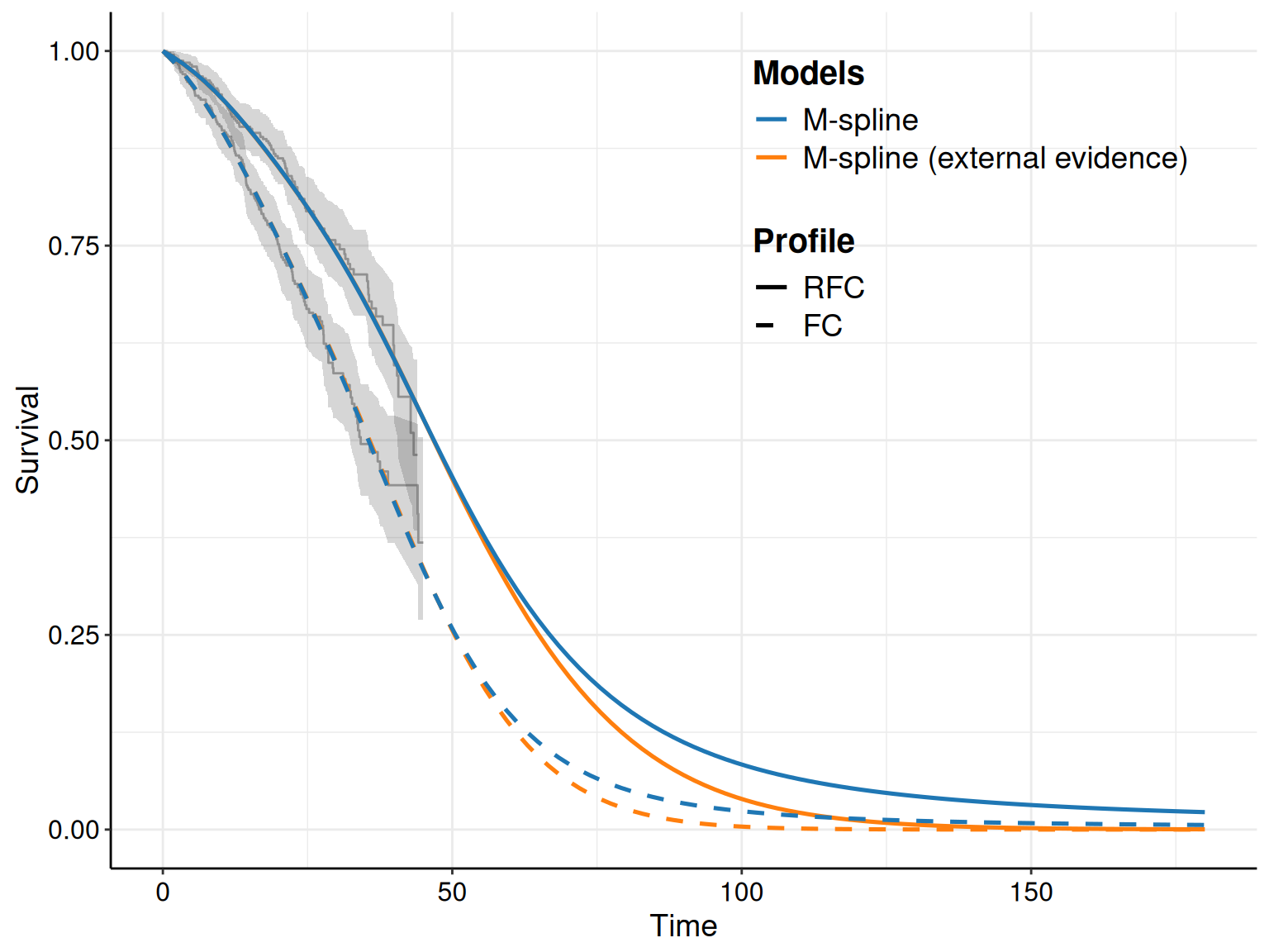
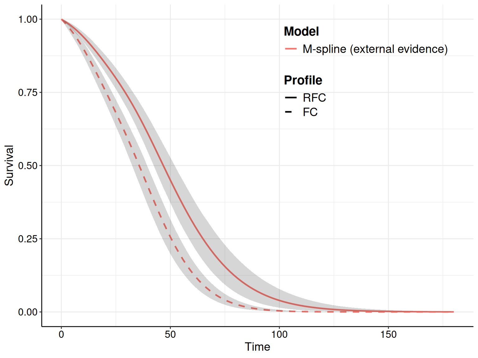
As is possible to see, the model using external data gets pulled towards 0 at later times (i.e. during the extrapolation part). Interestingly, the extra information also contributes to lower uncertainty (compare for instance Figure 8.13 (a) with Figure 8.12 (d)).
Another recent way of incorporating formally external information into the survival modelling is the “blended survival model” of Che et al. (2023), implemented in the R package blendR (available from CRAN, with a development version at the GitHub repository https://github.com/StatisticsHealthEconomics/blendR).
The main idea is to consider two separate processes. The first one is a model driven exclusively by the observed data; this is the same as the “standard” HTA analysis described above and is used to estimate \(S_{obs}(t\mid\boldsymbol\theta_{obs})\), with the aim of producing the best fit possible to the observed information.
Note that, unlike in standard modelling, we are not (too) concerned with overfitting, because we also consider a second process, which is used to derive a separate survival curve, \(S_{ext}(t\mid \boldsymbol\theta_{ext})\) to describe the long-term estimate for the survival probabilities. This may be based on “hard” evidence (e.g. real world evidence, registries, or cohort studies), or purely subjective knowledge elicited from experts (as described in Example 8.12) – or even both.
The two processes are “blended” together as \[ S_{ble}(t\mid\boldsymbol\theta) = S_{obs}(t\mid\boldsymbol\theta_{obs})^{1-\pi(t; \alpha, \beta, a, b)}\times S_{ext}(t\mid\boldsymbol\theta_{ext})^{\pi(t;\alpha, \beta, a, b)}, \] where \(\boldsymbol\theta = \{\boldsymbol\theta_{obs}, \boldsymbol\theta_{ext}, \alpha, \beta, a, b\}\) is the vector of model parameters; the weight function \[ \pi(t;\alpha,\beta,a,b) = \Pr\left(T\leq \frac{t-a}{b-a}\mid \alpha, \beta\right) = F_{\text{Beta}}\left (\frac{t-a}{b-a}\mid \alpha, \beta \right) \] controls the extent to which \(S_{obs}(\cdot)\) and \(S_{ext}(\cdot)\) are blended together in the blending period \([a,b]\); and \(t \in [0,T^*]\), is the interval of times over which we want to perform our evaluation.
This is not dissimilar to “mixture cure model” (De Angelis et al., 1999; Latimer and Rutherford, 2024), in which we assume that the underlying population is in fact made up by individuals who respond to treatment (and become “cured”) and others who do not as much (“uncured”), with a resulting mixed survival curve to model heterogeneity in the population. Conversely, in blended survival short- vs long-term processed are modelled explicitly with smooth transition and the main objective of extrapolation.
8.5.3 Network meta-analysis for survival data
In line with the discussion in Chapters 6 and 7, in HTA we often cannot access individual-level data for all the relevant interventions we need to compare. In the case of survival analysis, aggregated summaries typically consist of reported estimates for the (log)HRs, together with a measure of variability (e.g. a standard deviation).
We can expand the ideas of Chapter 7 to the case of survival outcomes, to make a suitable model that can pool together the “data” on the HRs (see Dias et al., 2018, chap. 10; Jackson et al., 2025). For example, the summary statistics for study \(s=1,\ldots,S\) typically consist an estimated log HR, \(y_{sa}\), defined for treatment arm \(a=1,\ldots,A\) against the reference arm considered in that study, with variance estimated as \(v_{sa}\).
Perhaps the simplest model in this situation is to consider \(y_{sa} \sim \text{Normal}(\mu_{sa},\, v_{sa})\), where \(\mu_{sa}\) is the true underlying log HR. Under a random effects specification, we have \[ \mu_{sa} \sim \text{Normal}(\delta_{sa},\, \sigma_\mu^2) \qquad \text{and} \qquad \delta_{sa} =d_a - d_{b_s}. \] Here, \(d_a\) is the pooled log HR for treatment \(a\) relative to the reference (\(d_1=0\), by convention) and \(b_s\) is the reference arm of study \(s\). The parameter \(\sigma_\mu^2\) is the between-study heterogeneity variance. In a Bayesian context, the model is completed by placing suitable priors on the parameters \(d_a\) and \(\sigma_\mu\).
This model produces posterior estimates of all pairwise log HRs across the network, which can be used to estimate the underlying survival curves. Assuming we have at least one ILD (possibly based on digitised data – see Section 8.3.2 for more details) to estimate the baseline hazard, one way to do so is to expand the M-spline model of Equation 8.13. Under the PH assumption, we model \[ h_a(t \mid \boldsymbol\theta) = h_0(t \mid \boldsymbol\theta)\exp(d_a). \] and then use Equation 8.6 to derive an estimate of the resulting survival curves.
When PH is implausible (e.g. for immunotherapies with delayed separation of survival curves), treatment effects can instead be introduced at the level of the spline coefficients \(\boldsymbol\omega\), allowing the log HR to vary smoothly over time, as described in Phillippo et al. (2024). The package multinma (Phillippo, 2024) can be used to run this sort of NMA.
8.6 Conclusions
This chapter has presented a long account of the intrinsic complexities associated with modelling time-to-event in HTA and the potential advantages produced by using the Bayesian approach. This is specifically related with the nature of the data, which is almost invariably characterised by limited follow-up and large censoring, which implies a lack of real information. This in turn makes the objective of extrapolation over a (much) longer time horizon, which is key to the HTA application, extremely complex and is particularly helped by the Bayesian feature of allowing a principled combination of different sources of information (be it prior knowledge, or additional data).
We have presented more “basic” parametric models and their use in survHE, as well as more “advanced” and flexible ones, through the use of survextrap. Both packages are based on a different MCMC algorithm (Hamiltonian Monte Carlo, see Section 2.3.3) – another consequence of the underlying complexity of modelling this sort of data, which renders computation more convoluted (and thus best effected using the, in this case, more efficient HMC).
The next chapter concentrates on so-called Markov models, another important tool that is very popular in HTA, which is used to describe the natural history of a specific condition by using a simulation approach for a “virtual” cohort of individuals. This sort of modelling tool is particularly helpful for economic modelling and has close links with survival analysis.
Technically, this is only one of the possible forms of “censoring”, indicated in the literature as “right censoring”. As this is the most common for applications in HTA, we limit our attention to it, here.↩︎
Actually, in the author’s considered opinion, being Bayesian is always time well spent…↩︎
It is possible to run the “hidden” function
survHE:::load_availables()to see all the available distribution names and the relevant abbreviation for each inferential engine.↩︎