This chapter expands mainly on concepts discussed in Chapter 5, when showcasing the use of Bayesian modelling for individual-level data in HTA.
In particular, we consider two important extensions that are often critical in health technology assessment alongside clinical trials: missing data and the presence of “structural” values. With this we encompass situations in which the observed data are characterised by “strange” values, which make the statistical analysis less straightforward. Examples include excess of zero costs, or perfect health utility (associated with a value of exactly 1).
Gabrio et al. (2025) present an extensive review of both frequentist and Bayesian modelling to handle missing data in HTA. More generally, Daniels and Hogan (2008) and Daniels and Xu (2020) are excellent references describing various Bayesian modelling strategies to deal with missing data (in the more general context of statistical modelling, rather than specifically in HTA).
In a nutshell, the problem with missing data is that we set out to observe \(n\) data points, but end up with a (much) lower number of fully observed individuals, \(n_{\text{obs}}\). Of course, the fundamental issue is how much lower is the amount of data available – if the proportion of missingness is negligible, there is no point in agonising over it and we can just carry on with our modelling.
Conversely, if it is not (and often it is not!), then the next question to ask is whether it has a non-differential impact: are individuals in one treatment arm (or with a given exposure or individual characteristics) more likely to be missing? Is there a specific reason or explanation as to why data are not observed?
Of course, the very fact that information is not present when we originally planned to have it means that we cannot base all of our judgement and analysis on the empirical data – this is similar to the issues encountered in extrapolation (see Section 8.3); more importantly, this will have implications in terms of assessing how well a model does in terms of fitting, because, of course, information criteria based on the likelihood (see the discussion throughout Section 5.3) do not fully apply here – recall that the likelihood is conditional on the observed data and thus cannot tell us anything about data that are not observed.
The material and ideas presented and discussed in this chapter are far from exhausting and, in fact, they are purposely focused on providing a “bigger picture” idea of the main complexities and the possible advantages in using a full Bayesian approach to deal with them. Excellent and more comprehensive literature on the overall problem of handling missing data include van Buuren (2018), Little and Rubin (2019) and Carpenter et al. (2023).
10.2 Missing data mechanisms
Similarly to the discussion in Section 5.2.2, the main idea is to model jointly two relevant processes: the “Model of Analysis” (MoA) is the usual data-generating process in which we assume a set of relationships between observable data and unobservable parameters, while the “Model of Missingness” (MoM) describes the mechanism by which some of the observable data are, in fact, missing.
More technically, we can consider a set of data \(\mathcal{D}_i = (y_i, \boldsymbol{x}_i, \boldsymbol{m}_i)\), where: \(y_i\) is the main outcome variable; \(\boldsymbol{x}_i\) represents a (vector of) covariate(s); and \(\boldsymbol{m}_i\) is a (vector of) missingness indicator variable(s). In general, we could face a situation in which missingness impacts both or either \(y\) and \(\boldsymbol{x}\) and thus \(\boldsymbol{m}_i\) would include as many elements as there are variables subject to missingness. Of course, the more structured missingness our dataset presents, the more complicated our overall analysis. For the sake of simplicity and to fix ideas, we consider here the simpler case in which missingness only affects the outcome variable – this means that there is only one missingness indicator \(m_i=1\) if \(y_i\) is not fully observed and \(m_i=0\) if it is.
Under the simplified scenario in which missingness only affects the outcome, another way to describe the data is to subset \(\boldsymbol{y}=(\boldsymbol{y}^{\text{obs}},\boldsymbol{y}^{\text{mis}})\), where \(\boldsymbol{y}^{\text{obs}}=(y^{\text{obs}}_1,\ldots,y^{\text{obs}}_{n_\text{obs}})\) are the fully observed data (i.e. those indexes \(i\) for whom \(m_i=0\)), while \(\boldsymbol{y}^{\text{mis}}=(y^{\text{mis}}_1,\ldots,y^{\text{mis}}_{n_\text{mis}})\) are those subject to missingness and thus for whom \(m_i=1\). Naturally, \(n=n_{\text{obs}}+n_{\text{mis}}\) is the overall sample size. The notation can be extended in the case of more structured missingness, e.g. also involving the covariates.
where the whole set of model parameters can be partitioned as \(\boldsymbol\theta=\left(\boldsymbol\theta^{\text{MoM}},\boldsymbol\theta^{\text{MoA}}\right)\); we often assume that, for simplicity, the subsets \(\boldsymbol\theta^{\text{MoM}}\) and \(\boldsymbol\theta^{\text{MoA}}\) are distinct, but this may not be plausible (in which case, we may need to consider some form of correlation across them). In addition, the notation \([,\boldsymbol{x}]\) indicates that covariates may or may not be included in a particular distribution.
The factorisation in Equation 10.1 is often termed a “pattern-mixture model” (PMM, Little, 1993), while that in Equation 10.2 is referred to as a “selection model” (SM, Diggle and Kenward, 1994). PMMs define a marginal model for all possible missingness “patterns” and thus require the specification of the MoA conditionally on each – this may be more intuitive from a “causal” point of view, but may require a great amount of information. Conversely, SMs consider a marginal MoA (essentially, the one that we would use even in the absence of missingness) and then specifies a conditional model for the missingness mechanism. While both factorisations are viable, SMs are sometimes preferred because of the simpler way in which we can handle the MoA.
Broadly speaking, there are three potential mechanisms that we can use to explain how missingness is generated (Rubin, 1976). This is akin to the concept of “data-generating process” introduced in Section 1.1 and used throughout this book: it is about constructing a model that expresses our view in terms of relationships among suitable variables and how they influence the data we actually get to see (if only partially).
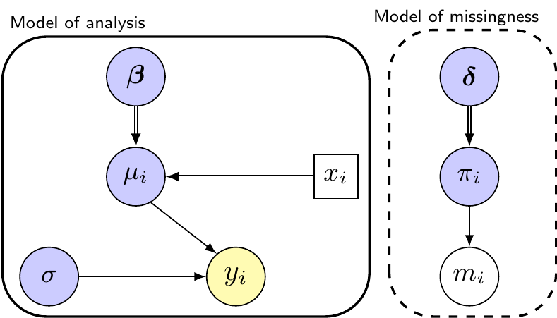
(a) MCAR.
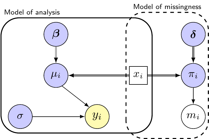
(b) MAR.
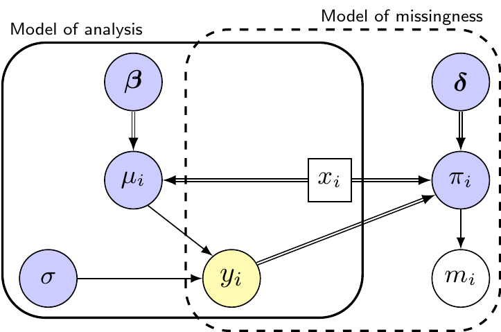
(c) MNAR.
Figure 10.1: Graphical representation of the common missingness mechanisms. Each panel shows the Model of Analysis, used to describe the overall data-generating process for the observable outcome, \(y\) and the Model of Missingness, which shows our assumptions on how missingness arises.
Figure 10.1 describes the three mechanisms using a SM representation. In each panel, the model parameters are shaded in dark colours and represented as circles; bold typesetting indicates that specific parameters may represent vectors. In addition, in line with Figure 3.1, double-edged arrows indicate logical relationships.
Unmodelled data (e.g. some covariate \(x_i\)), which we assume have been fully observed, are shown in a squared node with white background, while modelled data (e.g. the partially observed outcome \(y_i\) and the missingness indicator \(m_i\)) are also shown as circles – note that \(m_i\) is by necessity fully observed (because we know whether \(y_i\) is missing or not) and thus we represent it using a white background. Conversely, because we assume that \(y_i\) is subject to missingness, we depict it using a light coloured background.
In all panels, the solid boxes show the MoA, in this case defined, just to fix ideas, as a simple linear regression indexed by \(\boldsymbol\theta^{\text{MoA}}=(\boldsymbol\beta,\sigma)\)\[
\begin{aligned}
y_i & \sim \text{Normal}(\mu_i,\sigma) \\
\mu_i & = \beta_0 + \beta_1 x_i
\end{aligned}
\] – note that \(\mu_i\) is just a deterministic function of \(\boldsymbol\beta=(\beta_0,\beta_1)\) and \(x_i\) and thus we do not formally include it in \(\boldsymbol\theta^{\text{MoA}}\) above.
Similarly, the dashed boxes present the MoM, which describes the alleged sampling process for a missingness indicator \(m_i\). Without lack of generality, we can model \(m_i\sim \text{Bernoulli}(\pi_i)\), where \(\pi_i\) is the “probability of missingness”, typically centred at some value determined by \(\boldsymbol\delta\), e.g. on the logit scale.
Figure 10.1 (a) shows the “Missing Completely At Random” (MCAR) mechanism. This amounts to making the rather strong assumption that the two modules are completely separated, which implies that the way in which missingness is generated bears no impact on the model of analysis. Just to fix the ideas, we may use a simple model such as \[
\text{logit}(\pi_i) = \delta,
\] where the scalar \(\delta\) represents the average probability of missingness on the logit scale, common to all individuals.
Irrespective of the actual MoM, the key point here is the assumptions that \(\pi_i\) does not depend on the data \((y_i,x_i)\), or more prosaically that the MoA is independent on the MoM. Consequently, if this assumption is sensible (which it most often is not!), we can basically disregard the MoM and just carry on with our MoA as if missingness were not an issue: the estimates for the main parameters, i.e. \((\boldsymbol\beta,\sigma)\) in this case, will generally be unbiased – although they most likely will have lost precision, due to the lack of full information – see Example 10.1.
On a deeper level, the MCAR assumption also implies that we believe that the missing values occur just by total random chance and thus the value that we might have observed would have been generated by the exact same DGP that has produced the observed data.
Note 10.1: Complete case analysis and MCAR
Interestingly, when we analyse a dataset subject to missingness using standard statistical software, including R, the underlying (and often “silent”) assumption is exactly MCAR, as the following simple example shows.
# 1. Generates 100 data points for a covariate x ~ Normal(mean=2,sd=5)x=rnorm(100,2,5)# 2. Generates 100 data points for the outcome y, with :# a. intercept (beta0) = 0.5# b. "effect" of x (beta1) = 1.5# c. error variance = 1, ie add 'rnorm(100)', which simulates 100 # values from a Normal(0,1)y=.5+1.5*x+rnorm(100)# 3. Removes 20 values at random and replaces them with 'NA' (missing)y[sample(1:100,20)]=NA# 4. Runs a linear regression model (y on x) and print results summary(lm(y~x))
Call:
lm(formula = y ~ x)

Residuals:
     Min       1Q   Median       3Q      Max
-1.99584 -0.72194  0.02039  0.75906  2.29681

Coefficients:
            Estimate Std. Error t value Pr(>|t|)
(Intercept)  0.35741    0.10963    3.26  0.00165 **
x            1.46922    0.02241   65.58  < 2e-16 ***
---
Signif. codes:  0 '***' 0.001 '**' 0.01 '*' 0.05 '.' 0.1 ' ' 1

Residual standard error: 0.9493 on 78 degrees of freedom
  (20 observations deleted due to missingness)
Multiple R-squared:  0.9822,    Adjusted R-squared:  0.982
F-statistic:  4300 on 1 and 78 DF,  p-value: < 2.2e-16
Here, we simulate 100 data points \((y_i,x_i)\) and artificially remove 20% of the observations on the outcome \(y\), while retaining the original values for \(x\). The analysis performed by R using linear regression automatically considers only the “valid” cases (i.e. those completely observed on all the variables under consideration) – but note that other software such as Stata or SAS would proceed in exactly the same way. This method of analysis is often referred to as Complete Case Analysis (CCA), which is only valid if the underlying missingness generating mechanism is ignorable.
In fact, R explicitly tells us that it has deleted 20 observations (wasting the data on \(x\), which were available even for these individuals) due to missingness – a message that sometimes goes unnoticed by the analysts. In this case, the sample size is still large enough and the model estimates for the intercept \(\beta_0\) and the slope \(\beta_1\) are not “significantly” different from their “true” value (0.5 and 1.5, respectively).
In Figure 10.1 (b) we relax the rather unrealistic assumption of MCAR to consider the “Missing At Random” (MAR) mechanism: in this case, we assume that the probability of missingness does depend on the MoA, but only through the fully observed covariate \(x_i\), for instance through a logistic regression model \[
\text{logit}(\pi_i) = \delta_0 + \delta_1 x_i.
\] In other words, we believe that the pair \((m_i,x_i)\) includes all the information we need to determine the way in which missingness is generated. Pragmatically, this also means that, once we know the value of \(x_i\), the MoM becomes essentially irrelevant because, if we “control” for the important covariates, we do not need any further information to avoid bias in the estimates of the relevant parameters, e.g. \((\boldsymbol\beta,\sigma)\), in this case. This can be also shown in Figure 10.1 (b) as \(x_i\) “blocks” the pathway that connects \(y_i\) to \(\pi_i\).
As an example, consider some blood pressure readings in a patient. Empirical evidence suggests that this variable may be missing more often for older patients or women (e.g. because of scheduling issues or different clinic attendance patterns). In this scenario, indicating: the partially observed data as \(y_i\); the “true” value that would be observed if missingness had not occurred as \(y^*_i\); and the observed characteristics as \(\boldsymbol{x}_i=(\text{Sex}_i,\text{Age}_i)\), we then imply \[
\Pr(y_i \mid y^*_i,\boldsymbol{x}_i) = \Pr(y_i \mid \boldsymbol{x}_i),
\] or, in other words, that we believe that missingness in \(y_i\) is systematically related to observed patient characteristics \(\boldsymbol{x}_i\), but not the unobserved measurement itself (the true blood pressure, \(y^*_i\)).
Finally, in Figure 10.1 (c) we show what is most often the most likely description of the overall data-generating process, one in which the reason why an outcome is missing actually does depend on its unobserved value and termed “Missing Not At Random” (MNAR). In this case, the partially observed \(y_i\) also impacts on \(\pi_i\), for instance through a more structured logistic regression \[
\text{logit}(\pi_i) = \delta_0 + \delta_1 x_i + \delta_2 y_i.
\tag{10.3}\] In the blood pressure example, we may consider that patients with higher levels may be more prone to missing measurements because they are sick and, for that reason, cannot attend a scheduled clinic. In the case of MNAR, ignoring the MoM is not possible and if we do so the resulting estimates obtained for the model parameters will be biased – see again Example 10.1.
NoteThe data are…?
Sometimes, there is a tendency to abuse the language and use phrasing such as “we assume that the data are MAR”. This is not quite correct, because the data are just the data.
Much as they are not “Normal”, or “Gamma” (which are just models we are willing to adapt to describe our understanding of the underlying sampling variability inherent in the data-generating process), they cannot be MAR or MCAR or MNAR. These are just labels that we may be comfortable using to describe how we feel that the missingness has been generated.
For this reason, perhaps a better phrasing would be “we assume that the underlying missingness mechanism is MAR”. This is perhaps a mouthful and we may get away with the shortcut “the data are MAR” – but we should be fully aware of what that actually means…
Example 10.1. Missing data simulation study. We run a (ridiculously!) simple simulation study to demonstrate how different assumptions in the missingness mechanism can impact on the results of a model of analysis.
We start by considering a MNAR situation where the true MoM is \[
m_i \sim \text{Bernoulli}(\pi_i) \quad \text{with} \quad \text{logit}(\pi_i) = \delta_0 + \delta_1 x_i + \delta_2 y_i,
\] for set values \(\boldsymbol\delta=(\delta_0,\delta_1,\delta_2)=(-0.5, 0.35, 0.83)\). The actual numbers are not that important, but note that we imply a relatively large value for the impact of the outcome \(y\) on the probability of missingness \(\pi\) – recall the interpretation of the coefficients of a logistic regression after Equation 6.2 and Note 6.2 in Example 6.3.
As for the “true” relationship between \(y\) and \(x\), we imply a model \[
y_i = \beta_0 + \beta_1 x_i + \varepsilon_i \quad
\] in which we set the coefficients \(\boldsymbol\beta=(\beta_0,\beta_1)=(0.5,1.5)\) and \(\varepsilon_i \sim \text{Normal}(0,1)\). This is the same MoA of Note 10.1 above, but we consider a larger sample size of \(n=2000\) individuals to reduce the impact of sampling variability in the estimates.
We use the simple R code below to encode these assumptions and run the simulations.
# Initialisationmnar=list(); pmis=numeric(); S=1000; set.seed(140873)for (s in1:S) {# Simulates full data with a large sample size (n=2000) x=rnorm(2000,2,5) y=0.5+1.5*x+rnorm(2000)# MoM: MNAR (depends also on unobserved y) pi=bmhe::ilogit(-0.5+0.35*x+0.83*y) m=rbinom(2000,1,pi)# Creates missing data y[m==1]=NA# CCA analysis (ignores the MoM): saves estimates for the coefficients mnar[[s]]=(lm(y~x) |>summary())$coefficients[,"Estimate"]# Proportion of missing data in each simulation pmis[s]=sum(m==1)/2000}
Here, we first construct a large, fully observed dataset \((y,x)\) – note that we set the random seed, to ensure replicability. Then, we code the true MoM, in which we set the probability of missingness to depend on both the covariate \(x\) and the outcome \(y\), which we then set to NA according to this probability (or, equivalently, whenever \(m\) is equal to 1).
Finally, we analyse the data using a CCA, i.e. by simply letting the R function lm() remove the missing values, thus effectively ignoring the underlying MoM; note that although the CCA will discard the individual data affected by missingness, we use here the “correct” model – in reality, we may use a model that does not account for all the relevant factors (i.e. it is subject to residual confounding).
The estimated coefficients in each simulation are stored in the list mnar and this process is replicated for \(S=1000\) times. We also keep track of the proportion of missing data in the variable pmis: in this setup, the average proportion of missing data is around 65%. We can format the output into a tibble using the dplyr function bind_rows() so that we can apply the function bmhe::stats(), with which we compute some summary statistics, using the following command.
# Summarises the simulationsmnar |>bind_rows() |> bmhe::stats()
                mean         sd      2.5%    median     97.5%
(Intercept) 0.263245 0.05673721 0.1516397 0.2621029 0.3770304
x           1.457869 0.01344687 1.4301324 1.4579484 1.4833449
As is possible to see, in the long run, the estimates for both the intercept \(\beta_0\) and the slope \(\beta_1\) are not aligned with the “true” values (0.5 and 1.5, respectively): ignoring the informative missingness mechanism induces bias in our analysis.
Of course, if \(y\) had little influence on \(\pi\), the bias implied in the CCA may not be meaningful and essentially we would revert to a MAR situation, assuming \(x\)did have a substantive impact on \(\pi\) and we had controlled for it in our MoA. In fact, re-running the simulation study above setting pi=bmhe::ilogit(0.17+0.35*x+0*y) gives the following results.
MAR analysis
                 mean         sd      2.5%    median     97.5%
(Intercept) 0.5011553 0.04039917 0.4257231 0.5008061 0.5806213
x           1.4998349 0.00938082 1.4817550 1.4997070 1.5182100
This time, the simulation suggests unbiased estimates of both \(\beta_0\) and \(\beta_1\). Notice that we change the value of \(\delta_0\) in the linear predictor for the MoM from \(-0.5\) (used in the MNAR scenario) to \(0.17\), in order to keep consistency in the implied overall proportion of missing data, i.e. resulting in \(m_i=1\). We can use trial-and-error to tweak this parameter in order to achieve similar average values of pmis.
Similar results, with slightly increased precision, would hold if we re-defined pi=bmhe::ilogit(0.5+0*x+0*y). This would set the impact of \(x\) to 0 and the intercept \(\delta_0\) to 0.5 (again, we can use trial-and-error to identify a suitable value to keep a similar proportion of missingness), thus implying a MCAR mechanism.
MCAR analysis
                 mean          sd      2.5%    median    97.5%
(Intercept) 0.4991814 0.040756329 0.4176532 0.5011247 0.577936
x           1.5002119 0.007355783 1.4855884 1.5001326 1.514239
Interestingly, if we modified the simulation to fix pi=rep(0,2000) to produce no missing values and replicated the analysis, the results would obviously present more precision in the estimates – note the progressive reduction in the standard deviation of the estimates, particularly in comparison to the MNAR and MAR cases shown above (about 3 times as large and more than double, respectively, for the slope).
No-missing analysis
                 mean          sd      2.5%    median     97.5%
(Intercept) 0.4995238 0.024870810 0.4481647 0.4993299 0.5458013
x           1.5000762 0.004445692 1.4917870 1.4999367 1.5085892
While the results presented in Example 10.1 intuitively confirms that we cannot simply analyse the MoA in the case in which we must assume MNAR, an important complication is that, because \(y_i\) is not fully observed, this model is not empirically identifiable. In particular, the parameter \(\delta_2\) cannot be estimated using the available data only. We return to this point in Section 10.3.2.
In addition, natural extensions to the models presented above adapt for when there are multiple fully observed covariates collected in a vector \(\boldsymbol{x}_i\). Conversely, when missingness affect the covariates too, the model becomes a bit more convoluted, because we need to expand the presentation above to consider separate (but possibly correlated) MoMs, one for each variable that is affected by missingness. While, in theory, this is a reasonably straightforward extension, in practice, we need to have a large amount of fully observed data from which we can learn about the missing values, as well as be willing to make potentially untestable assumptions on the MoMs.
10.3 Missing data analysis methods
The discussion in Example 10.1 indicates that we should try and avoid using a CCA as our MoA, for two reasons: firstly (and most importantly), because this would only return estimates that are not biased in the case where the underlying missingness mechanisms are MCAR or MAR. In practice, this assumption may just not hold, as we may have strong knowledge of factors affecting missingness, which may well be beyond our control. More generally, we should not discard uncritically the possibility that, in fact, a MNAR mechanism may be more appropriate.
Secondly, even in the event that we may be willing to assume a MAR mechanism, we would obviously lose precision in our estimation, due to the lower observed sample size generated by the missingness. Coupled with the inevitable sampling variation affecting the data collection, this will likely contribute to producing unsatisfactory inference.
Although there are various methods suggested in the literature to handle the presence of missing data (including those based on “weighting” – see Section 11.3), we focus here on the most popular alternative, Multiple Imputation” (MI), in Section 10.3.1 and its fully Bayesian counterpart, in Section 10.3.2.
10.3.1 Multiple imputation
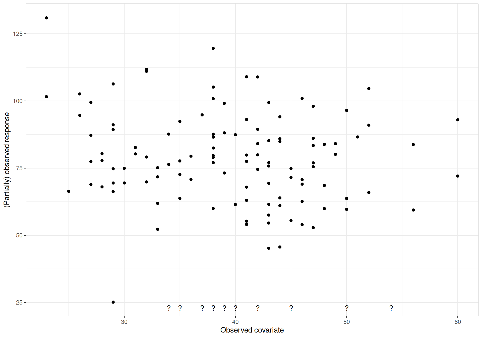
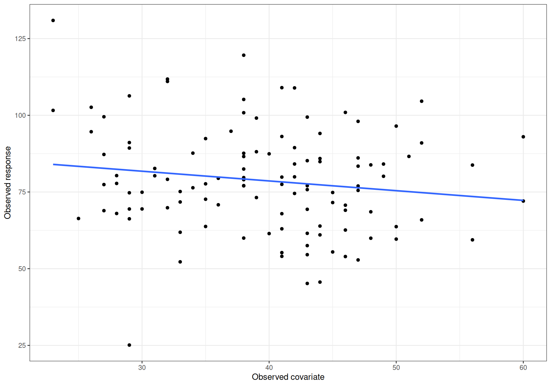
Suppose we observe a continuous variable \(y\) on \(n_{\rm{obs}} < n\) individuals; also, we completely observe an additional variable \(x\) on the \(n\) individuals in the sample. Figure 10.2 (a) shows the dataset, where fully observed individuals are represented as dots, while those for whom the outcome \(y\) is not known (but the covariate \(x\) is) are presented as ? along the \(x\)–axis.
If we can assume MAR, full knowledge of \(x\) is sufficient to “explain away” the MoM and thus we do not need to formally model it in our analysis. In Rubin (1977) and then in Rubin (1987), the main idea is that we can use the fully observed data to describe the underlying relationship between them. Of course, the simplest way in which we can do this is through a linear regression \[y_i = \beta_0 + \beta_1 x_i + \varepsilon_i \qquad \varepsilon_i \sim \text{Normal}(0,\sigma^2),\] to derive model-based estimates for the parameters \(\hat{\boldsymbol\theta}=(\hat{\beta}_0,\hat{\beta}_1,\hat\sigma)\). The resulting linear fit is shown in Figure 10.2 (b).
(a) (Partially) observed data for \(x\) and \(y\).
(b) Linear regression for the fully observed data.
(c) Multiple imputation.
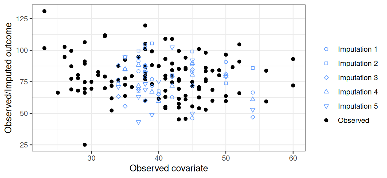
Figure 10.2: Graphical representation of the general principles underpinning multiple imputation. In panel (a) fully observed data are depicted as dots, while those for whom only the covariate on the \(x\)–axis is known are reported with a ? symbol. Under the assumption of MAR, in panel (b) the observed data are used to obtain predictions for the individuals for whom the covariate has been observed, but not the outcome. This is repeated a number \(R\) (\(=5\), in this case) of times to propagate uncertainty in the imputation, as shown in panel (c).
With these, we can also obtain a prediction for all the individuals for whom the outcome is missing as \[\hat{y}_i\sim \text{Normal}(\hat{\beta}_0 + \hat{\beta}_1 x_i,\hat\sigma^2).\] The estimates for \(\hat{\boldsymbol{\theta}}\) are obtained using the available data and thus are affected by the limited sample size (made even smaller by the presence of missingness), as well as the natural sampling variability. Consequently, a single prediction, or “imputation” in Rubin’s original terminology, is just not good enough to account for both the sampling variability in the partially observed data and the underlying uncertainty in the model parameters.
However, if we replicate this process for a (relatively small) number \(R\) of times, then we effectively can obtain \(R\) “complete” datasets, as shown in Figure 10.2 (c), where different symbols indicate the predicted value for \(y\) for each of the \(R=5\) imputations. We can then use each of these datasets to estimate the target quantities, e.g. the mean and standard deviation of the outcome, which we indicate as \((\bar{y}_r,s_r)\), for each imputation \(r=1,\ldots,R\), fitting a suitable model.
Once the estimates \(\bar{y}_r\) and \(s_r\) are obtained, then we can combine the \(R\) separate analysis results into a single final result, using “Rubin’s rule” \[\hat{\mu}_{\text{MI}} = \frac{1}{R}\sum_{r=1}^R \bar{y}_r\] with variance \[\hat{\sigma}^2_{\text{MI}} = \underbrace{\left(1 + \frac{1}{R}\right)}_{\substack{\text{finite sampling}\\ \text{correction}}}\underbrace{\left[\frac{1}{R-1}\sum_{r=1}^R \left(\bar{y}_r - \hat{\mu}_{\text{MI}}\right)^2\right]}_{\text{between imputation}} + \underbrace{\left[ \frac{1}{R}\sum_{r=1}^R s^2_r \right]}_{\text{within imputation}}. \tag{10.4}\]
This formulation accounts for the correlation across the imputations, thus producing unbiased estimates of the target quantities. More specifically, the within-imputation variance describes the average uncertainty that would arise even if there were no missing data, i.e. the sampling variability inherent in the process of analysing a complete dataset. On the other hand, the between-imputation variance reflects the extra uncertainty introduced by the limited information in our data, due to the missing values.
If the imputations are very different, then this factor is also large; more importantly, if we could construct infinity replications, then the within-imputation variance would vanish – thus the finite sampling correction is included to inflate the within-imputation variance, to reflect the extra uncertainty from only using \(R\) imputations to estimate the between-imputation variance. If \(R\rightarrow \infty\), then this factor disappears.
NoteThink like a Bayesian, do like a frequentist
Rubin’s ideas were very much grounded in a Bayesian perspective: the nature of multiple imputation is extremely similar to the simulation-based approach that characterises Bayesian modelling, of which Rubin himself has been a leading proponent, throughout his entire career.
Of course, back in the late 1970s and in the 1980s, researchers lacked both the computational power and the algorithms that have later allowed the “Bayesian revolution” of MCMC (see Section 2.3). Thus, his clever compromise was to “think like a Bayesian and do as a frequentist”: instead of looking for a large number of simulations (which was hard to obtain, even for simple linear regression models), he settled for a limited number of complete datasets (typically 5 to 10 replicates) and then use meta-analytic techniques to pool the estimates together – again, a more Bayesian way to do this would perhaps be to apply a full hierarchical version of the model as in Section 6.2.3: each complete dataset statistics \((\bar{y}_r,s_r)\) could be used as “data” and a model constructed to pool them and obtain a single estimate.
In reality, since the computational advancements of MCMC, there is no need to keep the Bayesian/frequentist compromise, but the practice has stuck and “multiple imputation” has remained the gold standard in missing data analysis methods.
In principle, we do not need to restrict the MoA to a linear regression and could use different link functions \(g(\cdot)\) for the linear predictor. It is also possible to relax MAR and produce versions of multiple imputation that, with some additional and typically untestable assumptions, can cater for MNAR. In any case, when relaxing the vanilla implementation of MI, the computational complexity of the “standard” hybrid imputation models increases substantially, thus suggesting that the marginal costs of implementing a full Bayesian version of the analysis is in fact decreasing. This is particularly relevant for the case of HTA, as we discuss more in detail in Section 10.4.
The basic caveat underpinning the extension of MI to more complex missingness mechanism scenarios is that we must preserve the property of congeniality(Meng, 1994) between the MoM and the MoA – in other words, if the model we use to impute the missing data is not fully consistent with the underlying data-generating process, then we would still imply bias in the final estimates. This has been addressed in different ways in the literature and, from a frequentist perspective, often using “robust” estimators1.
10.3.2 Bayesian modelling for missing data
From a Bayesian perspective, congeniality is less crucial, because there are no two separate steps (imputation and analysis); instead, using a single, unified structure to model the MoM and the MoA allows us to naturally handle the uncertainty from both the components. Thus, if the MoM is ignorable (e.g. under MAR), we can simply define the MoA and consider the missing data points as unobserved values to be estimated using the predictive distribution.
In other words, if MAR holds (meaning that we are prepared to assume its validity), then running a simple JAGS model such as the one sketched below would automatically take care of the missingness problem, by estimating a large number of samples from the predictive distribution of the outcome \(y\). Passing data as NA instructs JAGS to do that calculation.
# Defines the data - the actual numbers do not matter here! # NB: `NA` indicates the missing values in the vector yx=c(1,2,3,4,5,6,7,8,9,10,...)y=c(1,NA,2,NA,3,4,NA,NA,5,6,7,...)model_mar=function() {for (i in1:n) {# MoA y[i] ~dnorm(mu[i], tau) mu[i] <- beta0 + beta1*x[i] }# Priors for beta0, beta1 and tau/sigma, e.g. beta0 ~dnorm(0,0.1); beta1 ~dnorm(0,0.1) sigma ~dexp(2) tau <-pow(sigma,-2)}# Runs the model in JAGS m=jags(data=list(y=y,x=x,n=length(y)),# Note that we monitor y - the missing values will be "imputed" automaticallyparameters.to.save=c("beta0","beta1","sigma","y"),model.file=model_mar,n.chains=2,... # Other settings)
When the MoM is non-ignorable, then it would need to be included formally in the full analysis – and more importantly, the impact of the partially observed data would need to be modelled. But in this case, being Bayesian does come alive as a very efficient way of doing things, as adding a (most likely subjective/informative) prior distribution, e.g. on the coefficient \(\delta_2\) in Equation 10.3 would help “make up” for the lack of full information in the covariate \(y\).
# Defines the missingness indicatorm=ifelse(is.na(y),1,0)model_mnar=function() {for (i in1:n) {# MoA y[i] ~dnorm(mu[i], tau) mu[i] <- beta0 + beta1*x[i]# MoM - *must* be explicitly modelled! m[i] ~dbern(pi[i])logit(pi[i]) <- delta0 + delta1*x[i] + delta2*y[i] }# Priors for beta0, beta1, delta0, delta1 and sigma/tau: can be vague beta0 ~dnorm(0,0.1); beta1 ~dnorm(0,0.1) delta0 ~dnorm(0,0.1); delta1 ~dnorm(0,0.1) sigma ~dexp(2) tau <-pow(sigma,-2)# Prior for delta2: *must* use substantive information, e.g. delta2 ~dnorm(0.28,44)}# Runs the model in JAGS m=jags(data=list(y=y,x=x,m=m,n=length(y)),# Note that we monitor y - the missing values will be "imputed" automaticallyparameters.to.save=c("beta0","beta1","delta0","delta1","delta2","sigma","y"),model.file=model_mnar,n.chains=2,... # Other settings)
In the code above, we expand the model to account for a MNAR mechanism. In the absence of full data on \(y\), the prior for \(\delta_2\)must include substantive information on the likely impact of the outcome on the missingness – here we use a \(\text{Normal}(\text{mean}=0.28,\text{sd}=44^{-0.5}\approx 0.15)\) to encode some relatively strong belief. As \(\delta_2\) is modelled on the logit scale, we can use simple MC analysis to derive that this implies an average OR for missingness of about 1.34 with a 95% interval of \([0.2; 1.78]\). This would imply that we are very confident about the fact that larger values of \(y\) would be associated with larger odds of missingness and that there would be very little chance of this relationship not being substantial (as the probability that \(\exp(\delta_2)=\text{OR}<1\) is tiny).
In addition, it is a good idea to include in the MoM as much information as possible: thus, if we had additional covariates we should add them to the linear predictor in Equation 10.3, as this would contribute to stabilise our inference and anchor it as much as possible to the available evidence. At the same time, we should always acknowledge that any inference would rely on the (generally) untestable assumptions we make about the effect of the missing data on the generation mechanism.
10.4 Missing data in HTA
The case of missing data in the HTA context is interesting because, in addition to all the “normal” complexity discussed above, there are other issues that must be taken into account, which contributes to both the computational as well as the conceptual aspects of the analysis.
Similarly to the discussion in Chapter 5, the first and perhaps biggest complication is the fact that we need to consider a bivariate outcome \((e,c)\), made by two components that can show substantial correlation and non-linearity – and, notably, missingness can occur in either or both the two outcomes.
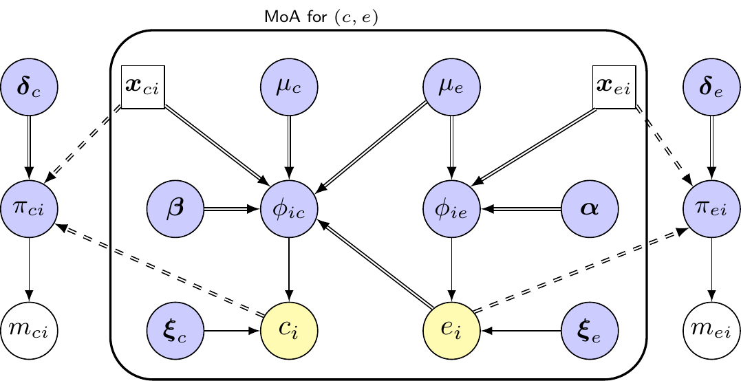
Figure 10.3 expands on the graphical representations presented above and provides a sketched version of the problem in the HTA context. Here, the MoA enclosed in the rounded rectangle embeds the marginal/conditional factorisation of the joint distribution \(p(e,c\mid\boldsymbol{\theta})=p(e\mid \boldsymbol\theta_e,x_{e})p(c\mid \boldsymbol\theta_c,e,x_{c})\) – see Section 5.2.2.
Figure 10.3: A (simplified) graphical description of the missingness mechanisms for a HTA problem. Here, dashed double-edged arrows indicate a logical relationship that may or may not be activated. For instance, the link between \(\boldsymbol{x}_{ci}\) and \(\pi_{ci}\) can be present only if we are willing to assume a MAR process for the costs; similarly the link between \(e_i\) and \(\pi_{ei}\) would be present if we were willing to assume MNAR for the benefits, but not otherwise. The colour coding of the nodes is the same as described in Section 10.2 and Figure 10.1. The box shows the MoA for the (partially) observed data on costs and benefits, while there are now two MoMs, one for the costs and one for the benefits (in the left- and right-most part of the graph, respectively).
However, we also must include the potential MoM components; this time, we need to allow for two mechanisms, one to explain the missingness for the benefits and the other for the costs – in Figure 10.3, these are the two sub-modules at either side of the graph. We may consider a simplifying assumption whereby the two missingness mechanisms are independent, but more likely we may imply some level of correlation, perhaps by considering common covariates, or even more formally by linking the two probabilities of missingness.
Various assumptions on the two mechanisms can be encoded by considering the following basic specifications: \[
\begin{aligned}
& m_{ei}\sim\text{Bernoulli}(\pi_{ei}); \qquad \underbrace{\underbrace{\underbrace{\text{logit}(\pi_{ei})=\delta_{e0}}_{\text{MCAR}} + \sum_{k=1}^K \delta_{ek}x_{eik}}_{\text{MAR}} + \delta_{eK+1}e_i}_{\text{MNAR}} \\
& m_{ci}\sim\text{Bernoulli}(\pi_{ci}); \qquad \underbrace{\underbrace{\underbrace{\text{logit}(\pi_{ci})=\delta_{c0}}_{\text{MCAR}} + \sum_{h=1}^H \delta_{ch}x_{cih}}_{\text{MAR}} + \delta_{eH+1}c_i}_{\text{MNAR}}.
\end{aligned}
\]
The inclusion of more covariates in the linear predictors defines different assumptions: if only the intercept \(\delta_{e0}\) or \(\delta_{c0}\) is included, then we are assuming a MCAR mechanism, while adding fully observed covariates extends to MAR and, finally, adding the missing outcome \(e\) or \(c\) encodes MNAR. Of course any combination is in theory possible, i.e. we could assume MAR or effects and MCAR for costs, or MNAR for effects and MAR for costs. As discussed earlier, in a Bayesian context, we would need to embed some subjective information in the priors for \(\delta_{eK+1}\) and \(\delta_{cH+1}\), to handle MNAR.
The multivariate and very structured nature of the modelling implies that in order to produce sensible results any form of MI must move away from simple and simplistic implementations, relying on Normality and independence. In turn, this suggests that the benefits of a full Bayesian approach may produce a very cost-effective alternative, particularly in light of the importance of the uncertainty analysis (which is even heightened in the face of limited information provided by the data).
Gabrio et al. (2025) present a thorough missing data analysis for the same TTT data discussed throughout Chapter 5 and we refer the reader that chapter as well as to the GitHub repository https://github.com/giabaio/R-HTA-code for more technical details and relevant R code.
10.4.1 Structural values
Another important quirk of HTA data is to do with the fact that the main outcomes may be subject to “structural values”. We use this terminology to indicate the case in which a variable is observed with an excess of specific values. A typical example is when individuals present with an assessment of perfect health, as captured by suitable scales (e.g. the EQ-5D). Another perhaps less intuitive example is when we observe total costs accrued equal to 0 – this may happen for instance when patients are so sick that they immediately exit the follow up without spending enough time under observation, or perhaps when they are substantially healthier than the rest of the population, thus failing to consume healthcare resources.
Either way, the fact that some individuals behave in a fundamentally different way than the rest of the target population may indicate the presence of distinct groups, leading to multimodality in the estimates for the average costs and benefits. Ignoring this mixture component typically will render the estimates biased and thus it is generally important to account for it in the modelling – particularly in presence of missing data.
Example 10.2. MenSS (adapted from Gabrio et al., 2019). The Men’s Safer Sex (MenSS) pilot randomised trial (Bailey et al., 2016) evaluates the cost-effectiveness of a new digital intervention to reduce the incidence of Sexually Transmitted Infections (STI) in young men with respect to the standard of care, involving no other active intervention. QALYs are calculated from utilities based on the EQ-5D 3L questionnaire (see Note 4.2 in Section 4.2), while the total costs are calculated from different components (but include no baseline value). x` The study was originally planned with sample sizes of \(n_1=75\) and \(n_2=84\) in the control and active treatment, respectively and Table 10.1 shows some summary statistics of the available data, across the various points in the follow-up. Over the course of the study, there is substantial drop-out, with only as little as 23% completing the observation (and thus providing full data) in the treatment arm.
Table 10.1: Summary statistics for the MenSS trial data. The study is initially planned with sample sizes of \(n_1=75\) and \(n_2=84\) in the control and active treatment, respectively. Source Gabrio et al. (2019).
Time
Type of outcome
observed (\%)
observed (\%)
Baseline
utilities
72 (96\%)
72 (86\%)
3 months
utilities and costs
34 (45\%)
23 (27\%)
6 months
utilities and costs
35 (47\%)
23 (27\%)
12 months
utilities and costs
43 (57\%)
36 (43\%)
Complete cases
utilities and costs
27 (44\%)
19 (23\%)
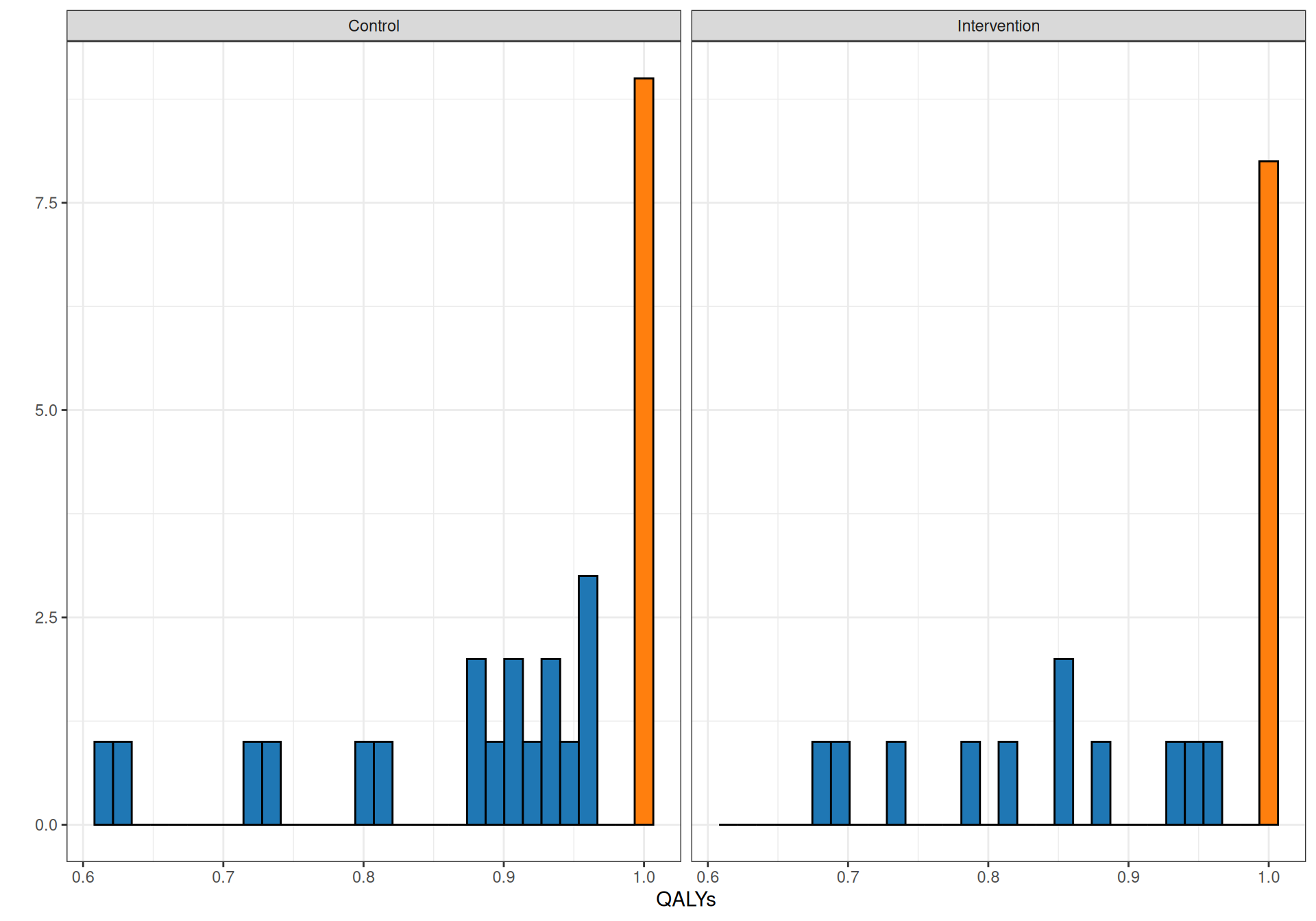
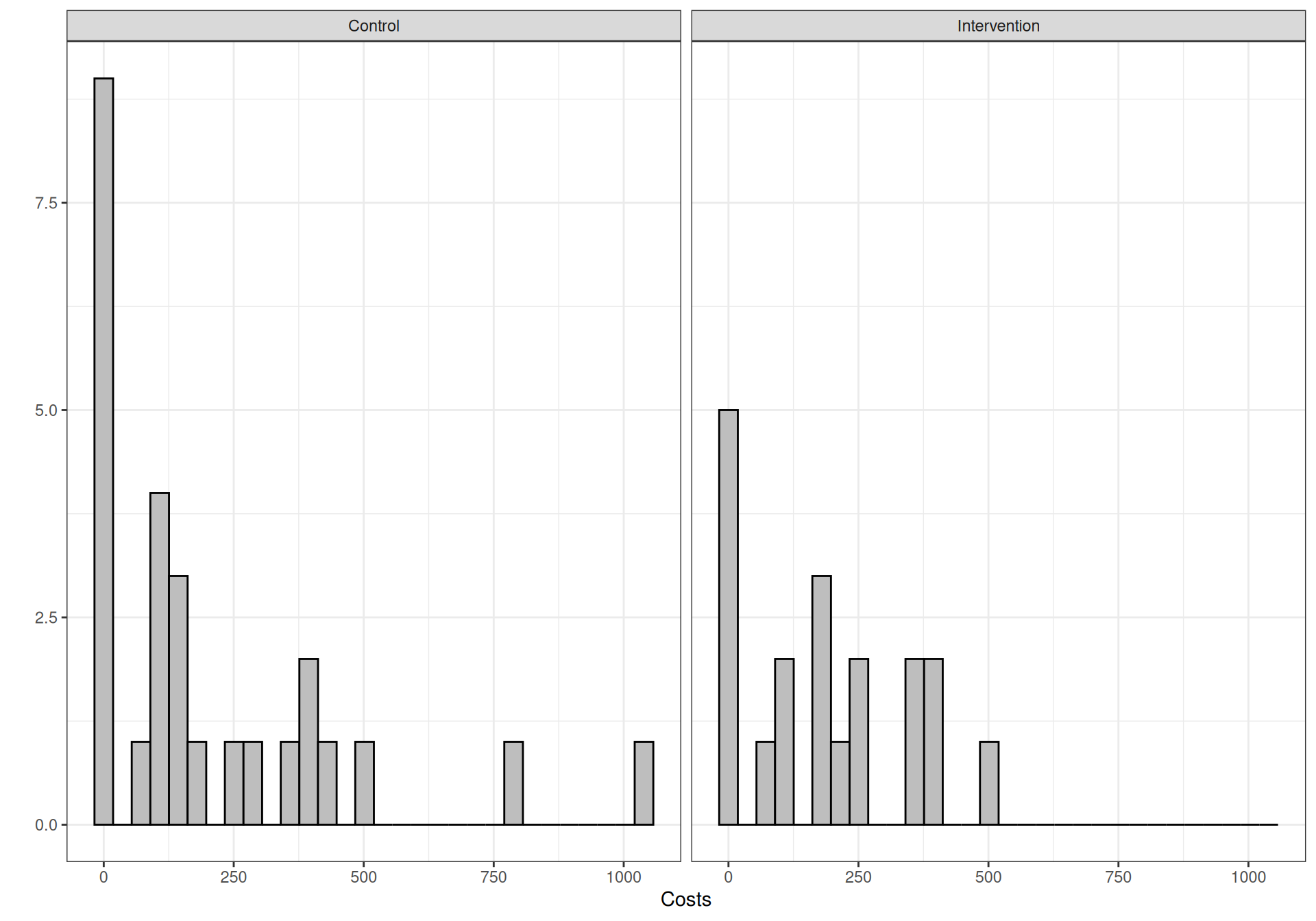
Figure 10.4 shows histograms for the distribution of QALYs and costs for the two treatment arms. As is possible to see, for both arms, the distribution of QALYs shows a marked “spike” at the value of 1, indicating a large proportion of participants in perfect health (the time horizon of the study is 1 year). This is not entirely surprising, given the nature of the study: the subjects are generally healthy and the underlying condition is typically not life-threatening.
Figure 10.4: Empirical distribution for QALYs and total costs in the two treatment arms of the MenSS trial. The lighter coloured bars in the top panel show the “spike” at the value of exactly 1.
From the statistical point of view, however, this generates further problems, in addition to the presence of substantial missing data. Given the annual time horizon of the study, the theoretical distribution of the QALYs is capped at 1 and thus we could model the observed data using a Beta distribution; the spike of values at exactly 1, however, violates this assumption, since the Beta distribution is defined in the open interval \((0,1)\).
Gabrio et al. (2019) compare three different models and present analyses for MAR and various MNAR assumptions. Here, we restrict our attention to the models assuming MAR for the effects and MNAR for the costs, for simplicity. This means that we assume that once the baseline utility values are observed, we can focus on the model of analysis and not worry about explicitly writing down further assumptions on the model of missingness. Of course, less restrictive (and more realistic!) assumptions would involve more complex modelling (see Gabrio et al., 2019; and Gabrio et al., 2025 for more detailed accounts).
The first model is a Normal-Normal MCF, similar to the one described in Example 5.3, in which the linear predictors are \[
\phi_{ei} = \alpha_0 + \alpha_1 \text{Trt}_i + \alpha_2 (u_{i}-\bar{u}) \qquad \text{and} \qquad \phi_{ci} = \beta_0 + \beta_1 \text{Trt}_i + \beta_2 (e_{i}-\mu_{et_{i}}),
\] where \(t_{i}=1,2\) identifies the treatment arm to which the \(i-\)th individual belongs.
The second model is a Beta-Gamma MCF. This is theoretically more appropriate, because it correctly recognises the natural range of the two variables – the interval [0-1] for the QALYs and the open positive real line \((0,\infty)\) for the costs. Here, we have \[
\text{logit}(\phi_{ei}) = \alpha_0 + \alpha_1 \text{Trt}_i + \alpha_2 (u_{i}-\bar{u}) \qquad \text{and} \qquad \log(\phi_{ci}) = \beta_0 + \beta_1 \text{Trt}_i + \beta_2 (e_{i}-\mu_{et_{i}}).
\]
While theoretically sound, this model has a fundamental, computational problem: the Beta distribution is constrained in the open interval \((0,1)\), which clashes with the observed spike at 1 for the QALYs. The simplest way to limit this issue is to subtract a small constant \(\varepsilon \rightarrow 0\) (say 0.01) to rescale all the QALYs, so that they actually can be modelled directly using a Beta. Note that this is possible because the observed range of the data is \([0.61; 1]\) and thus subtracting \(\varepsilon=0.01\) keeps all the values above 0.
This strategy is very easy to implement, but it feels a bit “hacky” and is potentially sensitive to the choice of the rescaling factor. In addition, much as the Normal-Normal MCF, it completely discards the fact that the observed spike may in fact indicate that the individuals have some fundamentally different features and thus the sampled data really are made by two potentially substantially different groups: the participants with \(\text{QALY}<1\), who experience some reduction in their QoL and those with perfect health.
We then develop a third model, based on a “hurdle” structure (Mullahy, 1986). The idea is to first model for each individual \(i\) an indicator \(d_{i}=1\) if \(e_{i}=1\) and 0 otherwise, using a logistic regression as a function of a set of relevant covariates \(\boldsymbol{X}_{i}\). Following Gabrio et al. (2019), we use age, ethnicity, employment status and the treatment arm to estimate the probability that a participant is a “structural one”, i.e. in perfect health, which is indicated as \(\gamma_{i}\).
Then, we treat as fixed the observed participants with \(\text{QALYs}=1\), while we model those with \(\text{QALYs}<1\) using a Beta distribution, without the need to rescale the values. For each treatment arm, the average effectiveness is then constructed as a mixture \[
\mu_{et} = (1-\bar\gamma_{t})\mu^{<1}_{et}+\bar\gamma_{t},
\] where \(\bar\gamma_{t}\) is the average probability of structural ones and \(\mu^{<1}_{et}\) is the average QALYs estimated for the data \(e^{<1}_{it}\), i.e. for the individuals with \(\text{QALYs}<1\). This comes directly from the Beta model, which we can fit with no complications, as this subset is indeed constrained in \((0,1)\).
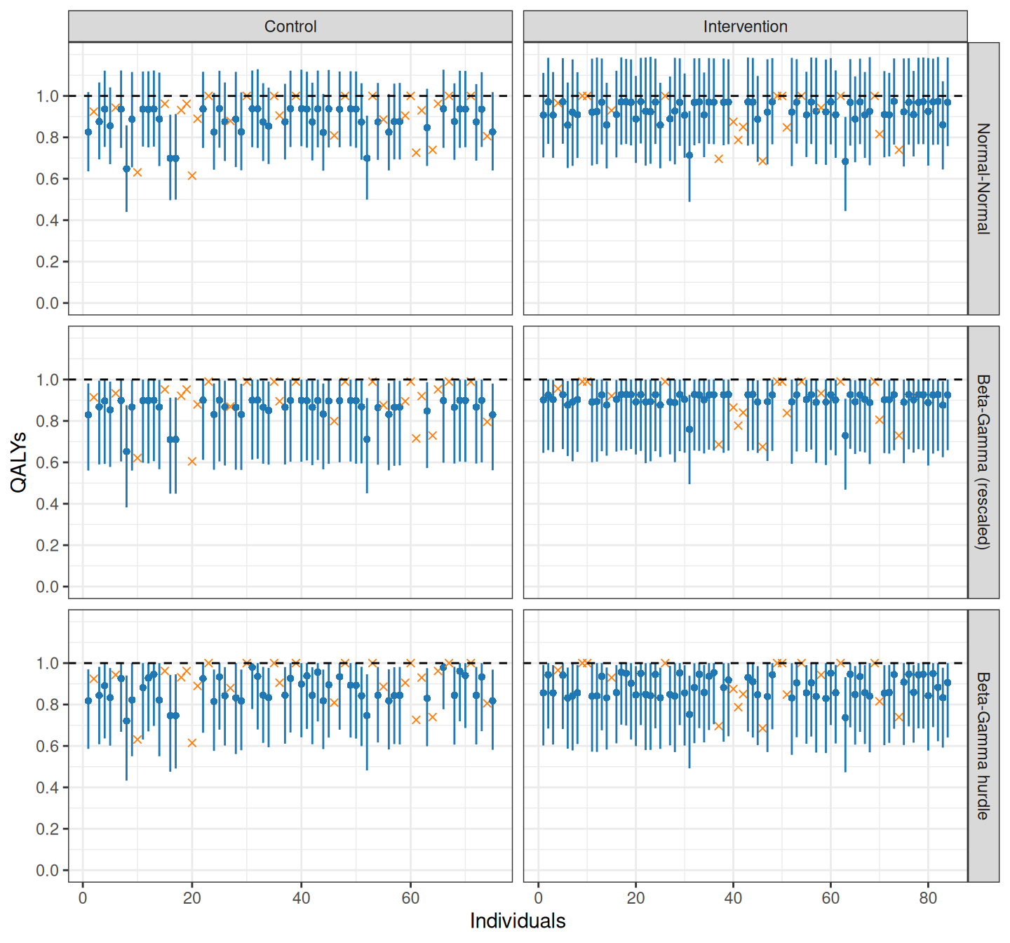
Figure 10.5 shows the results of the model, in terms of the “Bayesian multiple imputation”. Given the MAR assumption, the missing data are treated as unobserved values and are then sampled from the posterior predictive distribution.
In other words, the observed data and the assumptions in the model of analysis are used to first update the prior into the posterior distribution for the model parameters, which is in turn used to construct the posterior predictive distribution, averaging the sampling distribution \(p(e^{\text{mis}}\mid \boldsymbol\theta)\) with respect to the posterior \(p(\boldsymbol\theta\mid e^{\text{obs}})\) – see Equation 1.7.
Figure 10.5: Bayesian posterior predictive estimates for the distribution of the missing data. In each panel, the lighter crosses indicate the observed data, while dots and segments show the posterior predictive mean and 95% interval. The Normal-Normal MCF model is naturally unconstrained, which fails to conform with the nature of the QALYs (which should lay below 1). This holds for Beta-Gamma rescaled model, but the rescaling means that the estimates are all shifted down. The Beta-Gamma hurdle model can cater for all the idiosyncrasies in the data
In Figure 10.5, for the three models, the dots represent the posterior predicted average for the unobserved QALYs, while the segment covers the 95% interval of the predictive distribution. The lighter crosses indicate the observed data, for which we do not obtain a prediction (or imputation).
The first notable finding is that, as expected, the Normal-Normal MCF fails to account for the natural range of the data, producing predictions that span well beyond the upper limit of 1. This tends to inflate the overall mean effectiveness – basically, the Normal distribution does not know that that it should be bounded at 1 and thus artificially pushes up towards higher values, when the observation is large enough.
The Beta-Gamma (rescaled) model behaves much more nicely and is correctly capped at 1. Generally speaking, the estimates are not massively different, in terms of the means, although obviously the uncertainty is affected. However, more importantly, the crosses fail to recognise the individuals in perfect health – in the rescaled data, there is no such thing, which may introduce some slight downward bias in the overall average effectiveness.
Finally, the Beta-Gamma hurdle model gets around the idiosyncrasy in the data. Individuals in perfect health are modelled to determine their chance of in fact having a value of 1 for the QALYs. Those directly observed at 1 are correctly identified as such, but in addition those estimated to belong in this category are also modelled and estimated with a value of QALYs at 1.
10.4.2 Further complications
For all the implied complexity, the discussion above only scratches the surface of the many issues that can arise with missing data in HTA. One further potential complication is the fact that in principle the observed data on \((e,c)\) have in fact a longitudinal nature – in fact, the MenSS study is designed in this fashion.
While we often aggregate the longitudinal measurements into a cross-sectional summary, missingness may be “intermittent”, e.g. individals may be measured at baseline and at the first, but then not at the second follow-up, only to come back again at the third one. In a situation such as this, it is probably helpful to model these patterns and estimate the missing values at each time point in the follow-up – although, of course, this substantially complicates the modelling (see Gabrio et al., 2020; Mason et al., 2021).
From the computational point of view, the R package missingHE(Gabrio, 2024) simplifies the use of Bayesian modelling for missing data, based on JAGS code that is automatically created and run in the background, once the user specifies the main assumptions (on the missingness mechanism and the distributions for the partially observed data).
10.5 Conclusions
This chapter has given a very brief and sketched introduction to the philosophy underpinning statistical methods to deal with missing data, specifically for HTA. We have first reviewed the general mechanisms that we can use to describe the possible missingness generation and then moved to presenting typical modelling used to account for missingness in the analysis.
We have first discussed the gold standard of Multiple Imputation as a hybrid method – based on a Bayesian idea, but implemented within a frequentist approach. This was pretty much a historical accident, generated by the lack of suitable techniques that would allow a full Bayesian implementation.
Then, we have expanded to show how a Bayesian framework can be applied in general and specifically how it can prove particularly effective to deal with the several quirks of HTA data, including multivariate, non-Normal outcomes as well as structural values.
In the next chapter, we will discuss the ideas underpinning the principles of “population adjustment”, an increasingly popular extension to NMA methods (presented in Chapter 7).
Bailey, J., Webster, R., Hunter, R., Griffin, M., Freemantle, N., Rait, G., et al., 2016. The Men’s Safer Sex project: intervention development and feasibility randomised controlled trial of an interactive digital intervention to increase condom use in men. Health Technology Assessment 20, 1.
Carpenter, J., Bartlett, J., Morris, T., Wood, A., Quartagno, M., Kenward, M., 2023. Multiple Imputation and Its Application. John Wiley and Sons, Chichester, UK.
Daniels, M., Hogan, J., 2008. Missing Data in Longitudinal Studies: Strategies for Bayesian Modeling and Sensitivity Analysis. Chapman and Hall/CRC.
Daniels, M., Xu, D., 2020. Bayesian Methods for Longitudinal Data with Missingness, in: Lesaffre, E., Baio, G., Boulanger, B. (Eds), Bayesian Methods in Pharmaceutical Research. Chapman and Hall/CRC.
Diggle, P., Kenward, M., 1994. Informative drop-out in longitudinal data analysis. Journal of the Royal Statistical Society Series C 43, 49–73.
Gabrio, A., Daniels, M., Baio, G., 2020. A Bayesian parametric approach to handle missing longitudinal outcome data in trial-based health economic evaluations. Journal of the Royal Statistical Society Series A 183, 607–629.
Gabrio, A., Mason, A., Baio, G., 2019. A full Bayesian model to handle structural ones and missingness in economic evaluations from individual-level data. Statistics in Medicine 38, 1399–1420.
Gabrio, A., Mason, A., Leurent, B., Gomes, G., 2025. Missing Data, in: Baio, G., Thom, H., Pechivanoglou, P. (Eds), R for Health Technology Assessment. Chapman and Hall/CRC.
Little, R., 1993. Pattern-mixture models for multivariate incomplete data. Journal of the American Statistical Association 88, 125–134.
Little, R., Rubin, D.B., 2019. Statistical Analysis with Missing Data. John Wiley and Sons, New York, NY.
Mason, A., Gomes, M., Carpenter, J., Grieve, R., 2021. Flexible Bayesian longitudinal models for cost-effectiveness analyses with informative missing data. Health Economics 30, 3138–3158.
Meng, X.-L., 1994. Multiple-imputation inferences with uncongenial sources of input. Statistical Science 538–558.
Mullahy, J., 1986. Specification and testing of some modified count data models. Journal of Econometrics 33, 341–365.
Rubin, D., 1987. Multiple Imputation for Non-response in Surveys. Wiley.
Rubin, D., 1977. Formalizing subjective notions about the effect of nonrespondents in sample surveys. Journal of the American Statistical Association 72, 538–543.
Rubin, D., 1976. Inference and missing data. Biometrika 63, 581–592.
van Buuren, S., 2018. Flexible Imputation of Missing Data, 2nd ed. Chapman and Hall/CRC, Boca Raton, FL, USA.
A large emphasis is often placed on estimators being “doubly-robust” in the context of frequentist modelling of missing data. With this terminology, we generally indicate methods that remain valid (i.e. provide unbiased estimates) if either the MoM or the MoA is (reasonably) correctly specified – of course, as indicated in Note 5.1 in Section 5.3, no model can be completely “correctly specified”, but we can try to get as close as possible…↩︎