In the context of HTA, Markov models (sometimes referred to more generically as “Multistate models”, in the wider Statistical literature) are tools used to assess the long-term benefits and associated costs of a set of interventions, whose effect materialise on potentially repeating events (see Thom et al., 2025a; Thom et al., 2025b, as well as references therein for more details). The popularity of Markov models in HTA mainly derives from the fact that they are particularly effective at describing the “natural history of the disease” for many chronic conditions, which must be evaluated over a long enough time horizon.
Markov models are characterised by a set of relationships that identify the movement of a cohort of individuals across a number of “states”, or hypothetical outcomes that characterise a specific condition or disease. The way in which movements occur over time and across these states is determined by a set of relevant probabilities (or rates, in continuous time). A Bayesian approach can be particularly effective to model these probabilities, either from directly observed data or through evidence synthesis procedures.
In this chapter, we first give an introduction to the general “cohort Markov model in discrete times”. We do so by using a combination of data to feed into the estimation of the relevant probabilities and demonstrate the features of the tool in extrapolating the economic outcomes over longer time horizons, which again is a key feature for economic evaluation.
Then, we consider a specific case, the “Three-state cancer Markov model”, which is very popular and prevalent in much of the applications of HTA, combining this analysis with the methods described in Chapter 8.
9.2 Cohort Markov models
Generally speaking, we define a Markov model structure by considering a set \(\mathcal{S}\) made by \(S\) clinically relevant health states. These represent specific conditions or levels of the underlying pathology and are assumed to be exhaustive (i.e. they include all the relevant possible stages of the natural history of the disease) and mutually exclusive, meaning that if an individual is a state \(s=1,\ldots,S\) at time \(j=0,\ldots,J\), then they cannot also be in a different state \(s'\neq s\), at the same time.
From one period to the next, subjects can move among the states according to the rules specified by the Markov model’s assumptions. The movements occur according to suitable transition probabilities\[\lambda_{ss'} = \Pr(\text{individual is in state $s'$ at time }(j+1) \mid \text{individual was in state $s$ at time $j$}).\] The times \(j\) are often referred to as “Markov cycles” and a Markov model considers a “virtual follow-up” during which the cohort is free to move across the states.
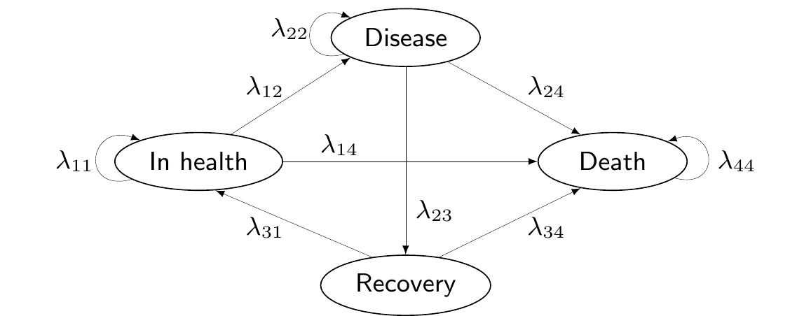
Figure 9.1 shows a graphical representation of a Markov model structure. Here, arrows indicate the possibility of moving from the state from which the arrow originates to the state in which the arrow ends. The absence of an arrow indicates that the transition between these nodes is not allowed.
Figure 9.1: A general graphical representation of a Markov model structure.
For instance, in Figure 9.1, we are assuming that individuals cannot move from the state “Recovery” back to “Disease”, without going through the state “In health” first. The state “Death” is an absorbing state – once individuals reach it, they cannot abandon it.
The assumption that the states are exhaustive and mutually exclusive implies that \[
\sum_{s'=1}^S \lambda_{ss'}=1.
\tag{9.1}\]
We can use some simple matrix algebra to fully characterise the Markov model in terms of the occupancy probabilities, describing the proportion of individuals who transition in each of the \(S\) states, at any given time. These can be obtained as \[\boldsymbol\pi_{j+1} = \boldsymbol\pi_{j} \boldsymbol\Lambda, \tag{9.2}\] where \(\boldsymbol\pi_j=(\pi_{j1},\ldots,\pi_{jS})\) is the vector of probabilities for each state at time \(j\) and \[
\boldsymbol\Lambda = \left(\begin{array}{c} \boldsymbol\lambda_{1} \\ \vdots \\ \boldsymbol\lambda_{S} \end{array} \right) = \left(\begin{array}{ccc}\lambda_{11} & \ldots & \lambda_{1S} \\ \vdots & \ddots & \vdots \\ \lambda_{S1} & \ldots & \lambda_{SS} \end{array}\right)
\] is a transition matrix, describing the probability of moving from state \(s\) to state \(s'\) at time \(j\). The vector \(\boldsymbol\lambda_s\) indicates the \(s-\)th row of the matrix \(\boldsymbol\Lambda\).
In this case, we imply that the transition probabilities do not vary over time – and thus for any Markov cycle \(j\), \(\lambda_{ss'}\) always indicate the probability of moving between the two states \(s\) and \(s'\) over two consecutive time points.
However in many cases the transition matrix should be allowed to vary over time (and would hence be indicated as \(\boldsymbol\Lambda_j\)); for instance, if the movements are affected by an individuals’ age, then the transition probabilities may vary in older ages (i.e. for later Markov cycles). Similarly, we may add a further index and write \(\boldsymbol\Lambda^{(t)}_j\), to indicate that the transition matrix changes for different treatment arms.
In the more general case where the transitions are allowed to vary over time, Equation 9.2 compactly computes the total probability of being in state \(s\) at time \(j+1\) as \[
\pi_{j+1\, s} = \pi_{j1}\lambda_{j1s} + \pi_{j2}\lambda_{j2s} + \ldots + \pi_{jS}\lambda_{jSs}.
\]
If we define \(m_{js}\) as the absolute number of individuals in state \(s\) at time \(j\), then we can also compute \[
m_{j+1\, s} = m_{j1}\lambda_{j1s} + m_{j2}\lambda_{j2s} + \ldots + m_{jS}\lambda_{jSs},
\] which we can again write in matrix algebra as \[
\begin{aligned}[t]
\boldsymbol{m}_{j+1} & = \, \boldsymbol{m}_{j} \boldsymbol\Lambda_j \\
(m_{j+1\, 1},\ldots,m_{j+1\, S}) & =\, (m_{j1},\ldots,m_{jS}) \left(\begin{array}{ccc}\lambda_{j11} & \ldots & \lambda_{j1S} \\ \vdots & \ddots & \vdots \\ \lambda_{jS1} & \ldots & \lambda_{jSS} \end{array}\right).
\end{aligned}
\tag{9.3}\]
In general, we can simulate a “virtual cohort” of individuals and their movements across the states for a period of time to evaluate the economic performance of a set of relevant interventions.
Example 9.1. HIV (adapted and expanded from Briggs et al., 2006). We consider the example originally discussed in Chancellor et al. (1997), also used in the description of the R package hesim(Incerti and Jansen, 2021), which can be used as a general framework for integrating statistical analyses with economic evaluation.
The economic evaluation considers two interventions for the treatment of HIV infection: zidovudine monotherapy (ZDV) and zidovudine + lamivudine in combination therapy (3TC+ZDV). The model includes 4 health states.
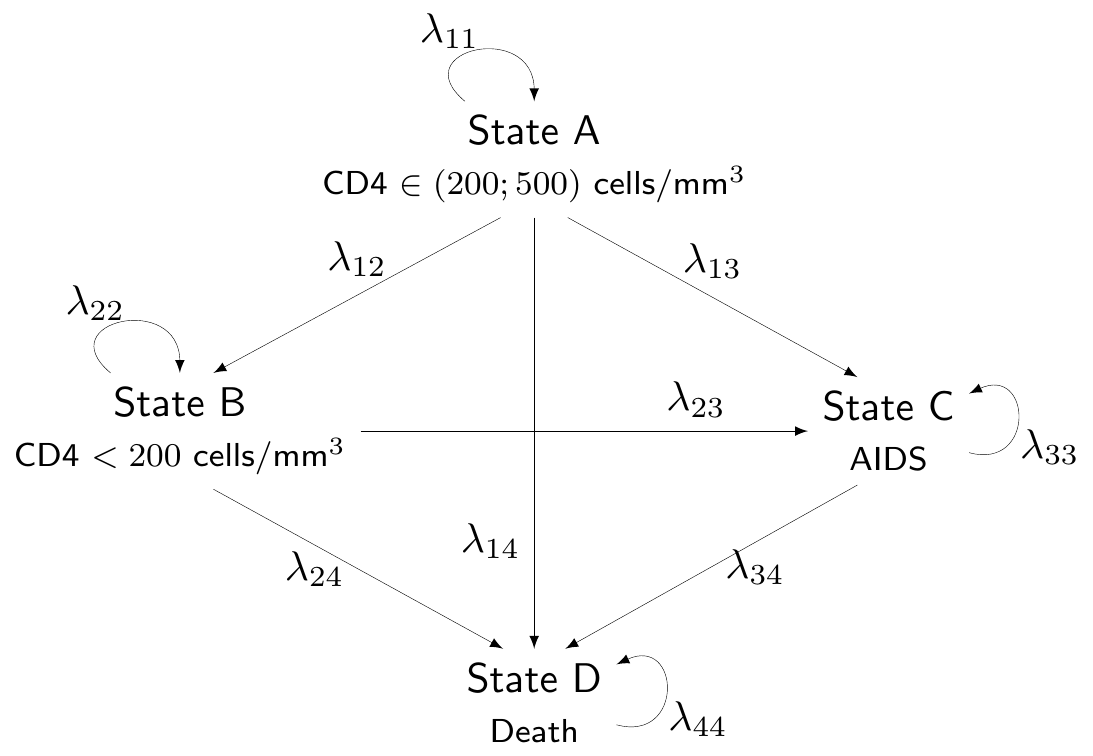
We label them as “State A” (HIV positive/non-AIDS with CD4 cells > 200 and < 500 cells/mm3, which we also label as “Compromised CD4”), “State B” (HIV positive/non-AIDS with CD4 < 200 cells/mm3, also labelled as “Low CD4”), “State C” (HIV positive/AIDS diagnosed, or “AIDS”) and “State D” (“Death”). This labelling indicates an implied ordering of severity of the underlying condition (so that A is less severe than B, which is less severe than C, etc.) and the model assumes only “forward” transitions, i.e. that patients can transition to any state that is more severe but cannot transition back to a less severe state.
Figure 9.2 shows a graphical representation of the modelling assumptions in terms of a DAG. For simplicity, we do not add a superscript \((t)\) to indicate that the transition probabilities are different in the two treatment options.
Figure 9.2: A graphical description of the assumptions embedded in the HIV Markov model. Source: Chancellor et al. (1997).
The simulation of the trajectories of patients across the \(S\) states is considered for \(J=20\) annual cycles, starting from \(j=0\).
9.2.1 Estimating the transition probabilities
While “running the Markov model” is reasonably simple and amounts to the basic matrix algebra defined by Equation 9.3, from the statistical perspective, the main complexity is in obtaining suitable estimates of the transition probabilities off each state, \(\boldsymbol\lambda_s\).
The simplest case is when we have observed data informing directly all the transitions. These amount to an \(S\times S\) matrix in which the number of movements between \(s\) and \(s'\) for all \(s,s'=1,\ldots,S\) are recorded over a suitable period of time. We can represent these data as \[
\boldsymbol{y}=\left(\begin{array}{c} \boldsymbol{y}_1 \\ \boldsymbol{y}_2 \\ \vdots \\ \boldsymbol{y}_S \end{array} \right) = \left( \begin{array}{cccc} y_{11} & y_{12} & \ldots & y_{1S} \\ y_{21} & y_{22} & \ldots & y_{2S} \\ \vdots & \vdots & \cdots & \vdots \\ y_{S1} & y_{S2} & \ddots & y_{SS} \end{array} \right),
\] where \[
n_s=\sum_{s'=1}^S y_{ss'} \qquad \text{and} \qquad \boldsymbol{n}=\left(\begin{array}{c} n_1 \\ n_2 \\ \vdots \\ n_S \end{array}\right)
\] is the vector of sample sizes.
We can reasonably describe the sampling variability characterising this particular data-generating process using a Multinomial distribution \[
\boldsymbol{y}_s \sim \text{Multinomial}(\boldsymbol\lambda_s, n_s) \quad \Rightarrow \quad p(\boldsymbol{y}_s \mid \boldsymbol\lambda_s )=\frac{n_s!}{\prod_{s'=1}^S y_{ss'}}\prod_{s'=1}^S \lambda_{ss'}^{y_{ss'}},
\tag{9.4}\] where \(\boldsymbol{\lambda}_s=(\lambda_{s1},\ldots,\lambda_{sS})\). Equation 9.4 can be seen as a multivariate generalisation of a Binomial distribution (cfr. Equation 1.16).
From a Bayesian perspective, we need a suitable probability distribution to model our epistemic uncertainty over \(\boldsymbol{\lambda}_s\). In the simplest of cases, we can assume \[
\boldsymbol{\lambda}_s \sim \text{Dirichlet}(\boldsymbol{a}_s) \quad \Rightarrow \quad p(\boldsymbol{\lambda}_s\mid \boldsymbol{a}_s)=\frac{\Gamma\left(\sum_{s'=1}^S \lambda_{ss'}\right)}{\prod_{s'=1}^S \Gamma\left( \lambda_{ss'} \right)}\prod_{s'=1}^S \lambda_{ss'}^{a_{ss'}}.
\tag{9.5}\]
The Dirichlet distribution is a multivariate generalisation of the Beta. Specifically, where the \(\text{Beta}(a,b)\) is a good model for a single parameter ranging between 0 and 1, the Dirichlet can be used to model \(S\) parameters \(\lambda_{s1},\ldots,\lambda_{sS}\) that are all constrained in the range \([0;1]\) and such that \(\displaystyle\sum_{s'=1}^S \lambda_{ss'} = 1\).
The parameters \(\boldsymbol{a}_s\) have a relatively intuitive interpretation, as they are proportional to the expected probability associated with the various outcomes. So if \(a_s\) is very large in comparison to the other parameters \(a_1,\ldots,a_{s-1},a_{s+1},\ldots,a_S\), then we are encoding the fact that outcome \(s\) is much more likely to occur than the others.
The scale of the parameters indicates the precision. So for example, in a \(S=3\)-dimensional case, a \(\text{Dirichlet}(1,1,1)\) encodes the assumption that the three possible categories are all equally likely (because the underlying parameters \(a_1,a_2,a_3\) are all the same). But in the same way, so would a \(\text{Dirichlet}(100,100,100)\), or for that matter a \(\text{Dirichlet}(0.01,0.01,0.01)\). In all cases the three parameters have the same value. The third distribution implies the lowest level of precision, while the second one implies large precision: intuitively, the larger the value, the more prior knowledge we consider.
Figure 9.3 shows six simplexes (which, in three dimension, are just triangles): each side of the triangles represents one of the Dirichlet parameters (in this case we assume an underlying variable with three possible categories).
(a) \(\boldsymbol{a}=(0.85, 0.85, 0.85)\).
(b) \(\boldsymbol{a}=(5, 5, 5)\).
(c) \(\boldsymbol{a}=(1, 2, 3)\).
(d) \(\boldsymbol{a}=(1, 7, 2)\).
(e) \(\boldsymbol{a}=(10, 5, 2)\).
(f) \(\boldsymbol{a}=(50, 50, 50)\).
Figure 9.3: Examples of a Dirichlet density on a 3d simplex. The lighter colours indicates areas of higher mass in the underlying distribution.
When \(a_1=a_2=a_3=0.85\) (Figure 9.3 (a)), the mass for the underlying Dirichlet distribution is spread all over the area in the triangle. This is the equivalent of a vague prior where the probability mass is spread all over the range of the variable.
Conversely, when \(a_1=a_2=a_3=50\) (Figure 9.3 (f)), the mass is concentrated in a small, central part of the triangle – intuitively, this means that the three dimensions carry the same weight (because the parameters have the same value); because that value is large, then the variance of the points is relatively low and thus the coloured part of the triangle (which indicates highest probability mass) is concentrated around the barycentre of the triangle.
When one of the dimensions has a much larger value than the others, the probability mass tends to be pulled towards that area, as happens when we consider a \(\text{Dirichlet}(10,5,2)\) in Figure 9.3 (e), where \(a_1\) is larger than both \(a_2\) and \(a_3\) and thus pulls the mass towards it. The remaining subfigures show different examples of Dirichlet distributions in which one of the three dimensions carries more weight than the others.
Just as the Beta distribution is related to the Binomial sampling distribution, so the Dirichlet is to the multivariate generalisation of the Binomial, i.e. the Multinomial distribution. Modelling a vector \(\boldsymbol{\lambda} \sim \text{Dirichlet}(a_{1},\ldots,a_{S})\) is the equivalent of the conjugated Beta-Binomial model (see Example 2.3) – i.e. with the added benefit that the posterior distribution given a vector of observed data \(\boldsymbol{y}\) is also a Dirichlet: \[\boldsymbol{\lambda}\mid \boldsymbol{y}\sim \text{Dirichlet}(a_{1}+y_1, \ldots, a_{S}+y_S). \tag{9.6}\]
Example 9.2. HIV (continued): Bayesian modelling. We can combine a number of data sources to estimate all the model parameters (including the transition probabilities) and then run the Markov model to perform the full economic evaluation.
Transition probabilities in the ZDV arm
We firstly set up the number of states \(S=4\). Also, we load the data, given in the form of matrices with the observed transitions across the states, during the actual follow-up in the trial. These are available for the control intervention (ZDV) The code is relatively straightforward – we use the R built-in function matrix() to define the data. Notice that the numbers included in the matrix are read by row (as the input byrow=TRUE suggests).
# Sets up the number of states and the names of the statesS =4states=c("Compromised CD4","Low CD4","AIDS","Death")y=matrix(c(1251, 350, 116, 17,0, 731, 512, 15,0, 0, 1312, 437,0, 0, 0, 469 ),ncol =4, nrow =4, byrow =TRUE)colnames(y)=rownames(y)=states# Row-wise sample sizen=apply(y,1,sum)# Visualises the data (observed transitions across states)y
                Compromised CD4 Low CD4 AIDS Death
Compromised CD4            1251     350  116    17
Low CD4                       0     731  512    15
AIDS                          0       0 1312   437
Death                         0       0    0   469
We can model the data \(\boldsymbol{y}_s\) using the Multinomial-Dirichlet structure described above – notice that, in this case, some of the cells in the transition matrix are fixed to 0 as not all transitions are possible.
In particular, we select a value of 3 for the scale parameter of the Dirichlet prior and define \(\boldsymbol{\lambda}_s \sim \text{Dirichlet}(\boldsymbol{a}_s)\), where \(\boldsymbol{a}_s\) is the \(s-\)th row of the matrix \[
\boldsymbol{A}= \left(\begin{array}{cccc} 3 & 3 & 3 & 3 \\ 0 & 3 & 3 & 3 \\ 0 & 0 & 3 & 3 \\ 0 & 0 & 0 & 3 \end{array} \right).
\] Combining this with the observed data guarantees that the inadmissible transitions (e.g. from “AIDS” back to “Compromised CD4”, governed by the parameter \(\lambda_{31}\)) are associated with probabilities identical with 0 (cfr. Equation 9.6). The posterior for the vectors \(\boldsymbol\lambda_s\) make up the full transition matrix for the ZDV arm, which we indicate as \(\boldsymbol\Lambda^{(1)}\).
Of course, other choices are possible – we use this a as a reasonably vague prior and explore sensitivity analysis to other configurations (noting that the sample sizes in the data are generally reasonably large). If covariates were available to inform the posterior distribution of \(\boldsymbol\lambda_s\), we could expand this model to use Multinomial-logistic regression (see for instance Lunn et al., 2013, pp. 129–132).
Relative risk of progression in the 3TC+ZDV arm
In this case, we do not have direct access to similar data for the “active” intervention (3TC+ZDV); however, Chancellor et al. (1997) consider a number \(L=4\) of relevant published studies in which the results of head-to-head comparisons (in terms of progression to fully established AIDS diagnosis) have been reported in the form of relative risks (RRs) and the resulting 95% interval estimates. These are reported in Table 9.1.
Table 9.1: Summary results of the relevant randomised clinical trials of 3TC vs ZDV. Source: Chancellor et al. (1997)
Study
Relative risk
95% CI
NUCA3001
0.389
0.206; 0.733
NUCA3002
0.674
0.393; 1.156
NUCB3001
0.492
0.183; 1.328
NUCB3002
0.452
0.226; 0.902
We can model these summary statistics to produce a pooled estimate for the RR and then apply it to the ZDV estimates for the transition probabilities, to derive the equivalent values for the 3TC+ZDV group. In particular, for each data point \(l=1,\ldots,L\), we use a partial pooling model (see Section 6.2.3) \[
\begin{aligned}
x_l = \log(\text{RR}_l) & \sim \text{Normal}(\theta_l,sd_l) \\
\theta_l & \sim \text{Normal}(\mu_\theta,\sigma_\theta) \\
\mu_\theta & \sim \text{Normal}(0,\text{sd}=2) \\
\sigma_\theta & \sim \text{Exponential}(2).
\end{aligned}
\]
Here, we first rescale the observed RRs using the log transformation – this makes the assumption of a Normal sampling distribution more plausible. Then, we derive an estimate of the individual study standard deviation as \[
sd_l \approx \frac{\log(\text{RR}^{upp}_l)-\log(\text{RR}^{low}_l)}{2 z_{0.05}},
\] where \(\text{RR}^{low}_l\) and \(\text{RR}^{upp}_l\) are the lower and upper limit of the 95% interval, respectively, while \(z_{0.05}\approx 1.96\) is the 97.5 percentile in the standard Normal distribution (see also Section 1.2.5).
We construct the partial pooling at the level of the mean RR, so that \(\rho=\exp(\mu)\) is the estimate for the pooled RR, across the four studies. We model \(\mu_\theta\) using a minimally informative Normal distribution, in which the prior sd of 2 implies that a prior 95% range of \([0.02; 50.4]\), on the exponentiated scale (as is easy to check using the properties of the Normal distribution).
Finally, we use a PC prior for \(\sigma_\theta\) – this implies that 95% of the prior mass lies below 1.5 (see Section 2.2.3), which is in fact a rather “relaxed” assumption, when translated on the natural scale for the RR.
Treatment effect waning
Chancellor et al. (1997) assume that the treatment effect lasts for exactly 2 years, after which all individuals revert to the same level as the ZDV arm. This implies that the RR is applied for the transition probabilities and that the costs of treatment are inflated by the acquisition of 3TC only for the first two Markov cycles. Nonetheless, they also acknowledge obvious uncertainty in this assumption by stating that “the extent of the duration of effect of 3TC/ZDV is not known, although surrogate marker data from trials NUCA 3001, NUCB 3001 and NUCA 3002 indicate that an effect persists for at least 1 year, and blinded follow-up data to week 76 suggest that effects may persist for closer to 2 years.”.
To account for this, here we construct a survival model for the treatment effect duration. We create pseudo-aggregated data in the form of Binomial counts to inform the proportion of people who would still be on active treatment effect after \(j\) (see Section 8.5.2).
For instance, we could imagine a situation such as that depicted in Table 9.2. Here, we pick \(I=8\) intervals, in correspondence of which we make informed guesses at the number of individuals who may reasonably still be under effective treatment (of course, in a “real” analysis, these guesses would be informed by clinical expertise and subject to thorough sensitivity analysis). In the table, the column labelled \(\delta\) shows the width of the discrete time intervals (e.g. \(\delta_1=0.5\) for the first interval, between times 0 and 0.5) and we encode the information provided in the original paper by assuming that very few events happen before 2 years and that by the end of year 3 the treatment effectiveness has waned off for everyone.
Table 9.2: Pseudo-data to encode the assumptions about the treatment effectiveness duration for the combination therapy
Interval
Width \( \delta \)
Events \(r\)
At risk \(nr\)
0 -- 0.5
0.5
0
100
0.5 -- 1
0.5
0
100
1 -- 1.5
0.5
3
100
1.5 -- 2
0.5
7
97
2 -- 2.5
0.5
60
90
2.5 -- 3
0.5
30
30
3 -- 4
1.0
0
0
4 -- 5
1.0
0
0
The observed counts in each interval are modelled as \(r_i \sim \text{Binomial}(\phi_i,nr_i)\), where \(nr_i\) is the number of people at risk. The parameter \(\phi_i\) indicates the probability that treatment wanes off, i.e. that it fails for at least one individual, in the \(i-\)th interval, which is equivalent to \(1-S_i\), the underlying interval-specific survival in effective treatment. Exponentiating and re-arranging Equation 8.6, we can write \(S_i\) in terms of the cumulative hazard \(H_i=h_i\delta_i\), where \(h_i\) is the hazard function in interval \(i\), which in turn allows us to express \[\phi_i=1-S_i = 1-\exp(-h_i\delta_i).\] If we assume that within each interval the underlying time-to-event is modelled with a \(\text{Weibull}(\alpha,\mu)\) sampling distribution, using the results in Table 8.4 and recalling Equation 8.3, we can write \[
\log(h_i) = \log(\alpha)-\alpha \log(\mu)+(\alpha-1)\log(u_i),
\] where \(u_i\) is the end point of the \(i-\)th interval. We can complete the model by setting suitable prior distributions for the Weibull parameters – for instance, we consider here \(\alpha,\mu\sim\text{Exponential}(2)\), independently, to provide reasonably vague priors.
Under this formulation, the pseudo-data \((r_i,nr_i)\) allow us to update the priors for \((\alpha,\mu)\) and with these we can construct for any time point \(j\) the survival curve \[
S(j) = \exp\left(-\left(\frac{j}{\mu}\right)^\alpha\right)
\] (cfr. again Table 8.4), which can be used to modulate the estimated RR from the evidence synthesis, by defining the time-varying RR \[
\rho^*_j = 1-S(j)(1-\rho).
\tag{9.7}\] Here, if \(S(j)\) is large (close to 1), then the actual, time-varying RR is close to \(\rho\). However, with smaller values of \(S(j)\), going down to 0 to indicate the point in time when the treatment effect completely wanes off, then the time-varying RR gets increasingly close to 1. Notice that while Equation 9.7 is linear both in \(\rho\) and \(S(j)\), it is highly non-linear in \(j\).
9.2.2 Rescaling transition probabilities
Once the posterior distribution for \(\rho^*_j\) becomes available, we can then combine it with the estimates from the Multinomial-Dirichlet component of the model to derive the time-varying transition matrix in the 3TC+ZDV arm – in theory, all we have to do is to multiply the baseline probabilities in \(\boldsymbol{\Lambda}^{(1)}\) by the time-varying relative risk \(\rho^*_j\).
In practice, however, things are more complicated than this simple multiplicative rescaling, for a number of reasons. Firstly, applying the RR to all the transition probabilities will break the sum-to-one constraint in each row of the resulting transition matrix for the 3TC+ZDV arm. This is relatively easy to overcome, for instance by considering a re-scaling of the resulting matrix such as the following. \[
\begin{aligned}
\boldsymbol\Lambda^{(2)}_{j} & = \boldsymbol\Lambda^{(1)} \rho^*_{j} + diag\left(1 - \sum_{s'=1}^S \lambda_{ss'}\rho^*_j \right) \\
& = \left(\begin{array}{cccc} 1-(\lambda_{12}+\lambda_{13}+\lambda_{14})\rho^*_j & \lambda_{12}\rho^*_j & \lambda_{13}\rho^*_j & \lambda_{14}\rho^*_j \\ 0 & 1-(\lambda_{23}+\lambda_{24})\rho^*_j & \lambda_{23}\rho^*_j & \lambda_{24}\rho^*_j \\ 0 & 0 & 1-\lambda_{34}\rho^*_j & \lambda_{34}\rho^*_j \\ 0 & 0 & 0 & 1 \end{array}\right).
\end{aligned}
\] To ensure that the rows of \(\boldsymbol\Lambda^{(2)}_{j}\) sum to 1, we add a diagonal matrix where the non-zero elements are equal to the quantity \(\left(1 - \sum_{s'=1}^S \lambda_{ss'}\rho^*_j\right)\). This is equivalent to adding this factor to the elements on the diagonal of the matrix \(\boldsymbol\Lambda^{(2)}_j\) only, which implies that: \(\lambda^{(2)}_{jss'} = \lambda_{ss'}\rho^*_j\), for \(s' \neq s\); and \[
\begin{aligned}[t]
\lambda^{(2)}_{jss} & = \lambda_{ss'}\rho^*_j + 1 - \sum_{s'=1}^S \lambda_{ss'}\rho^*_j \\
& = 1 - \sum_{s'\neq s} \lambda_{ss'}\rho^*_j \\
& = 1 - \sum_{s' \neq s} \lambda^{(2)}_{jss'},
\end{aligned}
\tag{9.8}\] as required.
However, in addition to this issue, there are other, potentially more subtle and complex quirks that we must be aware of when rescaling a vector of transition probabilities. One of the trickiest in a situation such as the one we are describing here is the fact that we want to “transport” an estimate for the RR obtained by a number of studies to our specific population, essentially under the following assumptions: i) that we only have a “control” arm available in our data; and ii) that our population is exchangeable (see Section 6.2.4) with the ones from which the pooled RR estimate is derived.
These two assumptions may be critical because, mathematically, two generic probabilities \(p_1\) and \(p_2\) are inextricably linked to a RR by the chain or relationships \[
\begin{aligned}[b]
\text{RR} = \frac{p_2}{p_1} & \Rightarrow 1 \geq p_2 = \text{RR}p_1 \\
& \Rightarrow \text{RR} \leq \frac{1}{p_1} \Leftrightarrow p_1 \leq \frac{1}{\text{RR}}.
\end{aligned}
\tag{9.9}\]
From a statistical point of view, however, when we “transport” the estimated distribution for RR onto our own study, we do not necessarily have a guarantee that Equation 9.9 holds for the baseline probabilities estimated from the data at hand (as in \(\boldsymbol\Lambda^{(1)}\) above).
Thus, if in the example above an entry \(\lambda_{ss'}>\frac{1}{\rho^*_j}\), then the resulting rescaled value for \(\lambda^{(2)}_{jss'}\) will exceed 1. Applying Equation 9.8 will still guarantee that the row-wise sum of the entries is 1, but some will be above 1 and others, by necessity, will be below 0, which is simply nonsensical. This mathematical impossibility should be taken as an indication that the assumption of exchangeability between the evidence synthesis data and our study is violated.
Finally, to avoid numerical instability in the resulting estimates, it may be helpful to work the problem on an unbounded scale. Considering again two generic probabilities \(p_1\) and \(p_2\) and the definition of RR, we can express \[
\text{OR} = \left.\frac{p_2}{1-p_2} \middle/ \frac{p_1}{1-p_1}\right. = \frac{p_2}{p_1}\frac{1-p_1}{1-p_2} = \text{RR}\left(\frac{1-p_1}{1-\text{RR}p_1}\right).
\tag{9.10}\] Therefore, recalling Equation 6.4 and using Equation 9.10, we can define \[
\begin{aligned}
\boldsymbol{\tilde{\Lambda}}_j^{(2)} & = \underbrace{\text{logit}^{-1}\left( \underbrace{\text{logit}\left(\boldsymbol{\Lambda}^{(1)}\right) + \log(\text{OR})}_{\text{rescales in }(-\infty;\infty)} \right)}_{\text{rescales back to }[0;1]} \\
& = \text{logit}^{-1}\left(\text{logit}\left(\boldsymbol{\Lambda}^{(1)}\right) + \log(\rho^*_j) + \underbrace{\log\left(1-\boldsymbol{\Lambda}^{(1)}\right) - \log\left(1-\rho^*_j \boldsymbol{\Lambda}^{(1)}\right)}_{\text{adjusts RR to derive OR}} \right) \\
& = \left(\begin{array}{ccc}\tilde{\lambda}^{(2)}_{j11} & \ldots & \tilde{\lambda}^{(2)}_{j1S} \\ \vdots & \ddots & \vdots \\ \tilde{\lambda}^{(2)}_{jS1} & \ldots & \tilde{\lambda}^{(2)}_{jSS} \end{array}\right)
\end{aligned}
\] and then compute \[
\boldsymbol{\Lambda}_j^{(2)} = \boldsymbol{\tilde{\Lambda}}_j^{(2)} + diag\left(1 - \sum_{s'=1}^S \tilde{\lambda}^{(2)}_{jss'} \right)
\tag{9.11}\] to ensure that the transition probabilities sum to 1 in each row of the resulting transition matrix. Again, if the assumption of exchangeability is broken and \(\boldsymbol\Lambda^{(1)}\) is not consistent with the estimated values for \(\rho^*_j\), even Equation 9.11 may produce nonsensical estimates for the transition probabilities in \(\boldsymbol{\Lambda}_j^{(2)}\) – but note that Equation 6.4 is not affected by this problem, which can occur because of the adjustment factor \(\log\left(1-\boldsymbol{\Lambda}^{(1)}\right) - \log\left(1-\rho^*_j \boldsymbol{\Lambda}^{(1)}\right)\).
Note also that, in the HIV example above, it makes sense to further rescale the elements on the diagonal of \(\boldsymbol{\Lambda}_j^{(2)}\) because the model assumes that only “forward” progressions are allowed – individuals can either remain in the current state, or progress to a more severe health state. But because the RR is specifically estimated to determine the effectiveness of 3TC+ZDV in preventing these transitions, it is reasonable to apply it to those probabilities and simply rescale the elements on the diagonal, which indicate the chance that an individual does not progress from the current state, to ensure that each row of the transition matrix sums to 1.
In other problems, this may be more complex and, in general, we need to be very careful about rescaling, when obtaining probabilities using procedures such as the one highlighted above.
Example 9.3. HIV (continued): Bayesian modelling (2). The original analysis in Chancellor et al. (1997) reports estimates for a set of relevant costs of care, as shown in Table 9.3.
Table 9.3: Cost estimates (in 1995 £). Source: Chancellor et al. (1997)
Mean cost per patient per year
CD4 \(\in[200; 500]\)
CD4 \(<200\)
AIDS
Direct care
1701
1774
6948
Community care
1055
1278
2059
In the original model, these are considered as fixed, although a scenario sensitivity analysis uses a set of alternative values for the cost of direct care (specifically set at 2938, 4398 and 11 223 for the three states respectively).
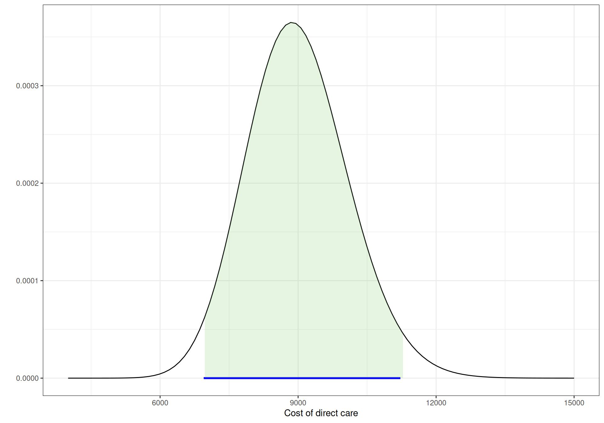
We instead use this information to build a model encoding the uncertainty over the cost of direct care. We use trial-and-error and the bmhe function gammaPar() (see Example 7.4) to get values for the parameters of a Gamma distribution for which most of the mass is approximately between the two extremes.
For example, we could use something like the following code (see Note 7.3 in Example 7.4 for more detail on using shortcuts for functions in R “pipes”).
# Trial and error to get the parameters of a suitable Gamma (approximately!)bmhe::gammaPar(2300,350) |> (\(x) rgamma(100000,shape=x$shape,rate=x$rate))() |> bmhe::stats()
     mean        sd      2.5%    median     97.5%
2298.0286  348.3423 1662.6982 2280.4296 3028.7837
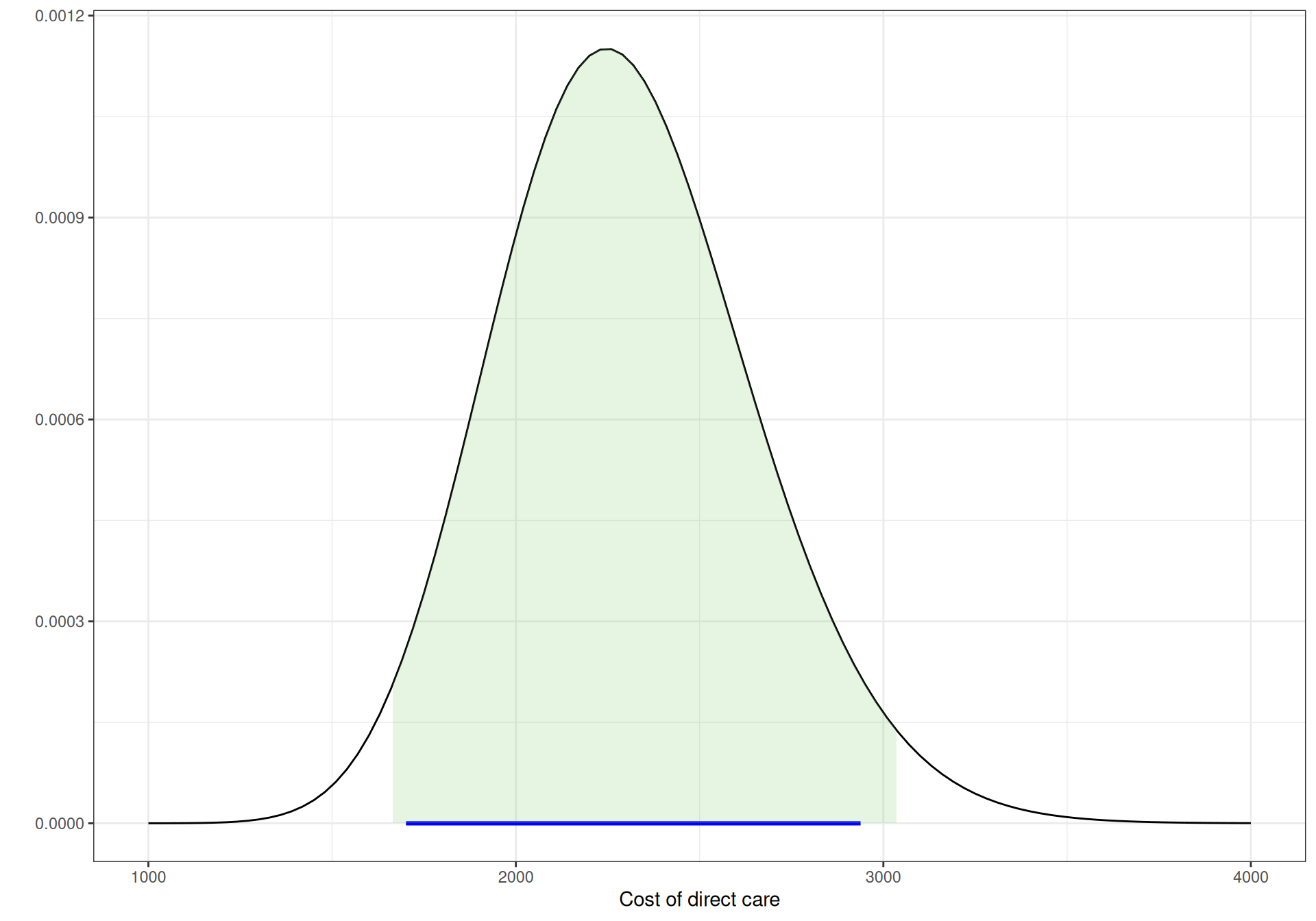
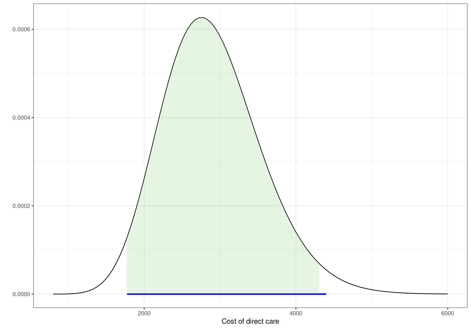
to obtain a reasonably close interval for a \(\text{Gamma}(43.184,0.019)\) distribution to model the cost of direct care in “Compromised CD4” with 95% of the mass approximately in the interval \([1701;2938]\). Similar calculations can be made for the other two states, to give \(\text{Gamma}(19.905,0.007)\) for “Low CD4” and \(\text{Gamma}(66.942,0.007)\) for “AIDS”.
Figure 9.4 shows graphically these three Gamma distributions. The horizontal segment below the \(x\)–axis indicates the observed extremes for the data, while the shaded area under the curves is the 95% interval under these priors. As is possible to see, all are pretty much aligned.
(a) CD4 \(\in [200; 500]\).
(b) CD4 \(<200\).
(c) AIDS.
Figure 9.4: Gamma priors for the cost of direct care.
The cost of community care is informed by the data presented in Table 9.3. Ideally, we would have hard evidence (and perhaps a combination of sources) to be able to account for some uncertainty around these estimates. In the absence of this, we could use expert knowledge to elicit some plausible range and then follow a similar mechanism as above to derive suitable parameters for a Gamma distribution. Alternatively (and somewhat less satisfactorily), often HTA practitioners tend to add noise to the mean estimates by setting the standard deviation to a fraction of the mean – see Example 7.4 for another example of this practice.
Here, we follow this strategy and set the standard deviations to 20% of the point estimates. Using again bmhe::gammaPar(), we find that \(\text{Gamma}(25,0.0237)\), \(\text{Gamma}(25,0.0196)\) and \(\text{Gamma}(25,0.0121)\) are suitable models for the states “Compromised CD4”, “Low CD4” and “AIDS”, respectively.
Finally, as for the acquisition of the two drugs, the cost of a year of treatment with ZDV is estimated at \(c_{\text{mono}}=\) £2278, while 3TC adds an annual cost of £2086. Chancellor et al. (1997) assume three deterministic scenarios for the cost of the combination therapy, dictated by the treatment effectiveness duration.
In the base-case scenario, the treatment effect is assumed to last for exactly 2 years, during which the annual cost of 3TC+ZDV is given by \(c_{\text{comb}}=\) £(2278 + 2086)=£4364. After that, patients switch back immediately to monotherapy at an annual cost of \(c_{\text{mono}}\), for the rest of the virtual follow-up (until \(J=20\) years). We take a similar approach, but consider an annual cost of \(c_{\text{comb}}\) for as long as the treatment effectiveness is estimated to be above 0, i.e. as a function of the survival curve \(S(j)\) defined above.
At this point, we can finally code up all the modelling assumptions into a suitable JAGS code and then run it to obtain the estimates for the posterior distributions. We can do so using the following code.
model=function(){# Multinomial-Dirichlet model for the observed transitions in the ZDV armfor (s in1:S) { y[s,1:S] ~dmulti(lambda[s,1:S],n[s]) lambda[s,1:S] ~ddirch(a[s,1:S]) }# Evidence synthesis for the RR in 3TC+ZDV vs ZDVfor (l in1:L) { x[l] ~dnorm(theta[l],prec.x[l]) theta[l] ~dnorm(mu.theta,tau) } mu.theta ~dnorm(0,0.25) sigma.theta ~dexp(2); tau <-pow(sigma.theta,-2) rho <-exp(mu.theta)# Treatment effectiveness durationfor (i in1:I) { r[i] ~dbin(phi[i],nr[i]) phi[i] <-1-exp(-h[i]*delta[i])log(h[i]) <-log(alpha) -alpha*log(mu) + (alpha-1)*log(u[i]) } alpha ~dexp(2) mu ~dexp(2)# Estimates time-varying RR with treatment effect waningfor (j in1:(J+1)) { surv[j] <-exp(-pow(((j-1)/mu),alpha)) rho.star[j] <-1-surv[j]*(1-rho) }# Model for the cost of direct care and for the cost of community carefor (s in1:(S-1)) { c.direct[s] ~dgamma(shape.dir[s],rate.dir[s]) c.comm[s] ~dgamma(shape.comm[s],rate.comm[s]) } c.direct[S] <-0; c.comm[S] <-0# Model for the annual cost of combination therapy c.comb[1] <- c.mono+c.3tcfor (j in2:(J+1)) { c.comb[j] <-ifelse(surv[(j-1)]>eps, c.mono+c.3tc, c.mono) }}
This code is fairly straightforward and modular. We first include the Multinomial-Dirichlet model for the observed data in the ZDV arm. Then, we perform the evidence synthesis on the four studies to estimate the RR of progression for the combination therapy. Next, we use the aggregated pseudo-data to model the treatment effect duration and use the resulting survival curve (the node surv, defined for each Markov cycle, \(j=0,\ldots,J\) and thus for a total of \(J+1\) points) to compute the time-varying RR, rho.star[j].
Finally, we model the various costs, taking care of setting the cost associated with the state “Death” to 0. Notice also that JAGS allows the use of a number of vector- and array-valued functions, much as R would do. In this case, we use the ifelse() function to define the cost of the combination therapy as a function of the treatment effectiveness, as mentioned above. Notice that we assume that the combination therapy fails whenever the estimated survival curve for the treatment effectiveness duration goes below a small threshold eps, set at 0.001 in the data list defined using the code below.
# Defines the data list and runs the modellibrary(R2jags)datalist=list(y=y,S=S,n=n,x=x,prec.x=1/sd^2,L=length(x),J=20,a=matrix(c(3,3,3,3,0,3,3,3,0,0,3,3,0,0,0,3),nrow=S,byrow=T),shape.dir=c(43.184,19.905,66.942),rate.dir=c(0.019,0.007,0.007),shape.comm=c(25,25,25),rate.comm=c(0.027,0.0196,0.0121),u=c(.5,1,1.5,2,2.5,3,4,5),r=c(0,0,3,7,60,30,0,0),I=8,nr=c(100,100,100,97,90,30,0,0),delta=c(0.5,0.5,0.5,0.5,0.5,0.5,1,1),c.mono=2278,c.3tc=2086,eps=0.001)hiv=jags(data=datalist,parameters.to.save=c("lambda","c.direct","rho.star","c.comb","c.comm","surv" ),model.file=model,n.chains=2,n.iter=10000,n.burnin=5000)
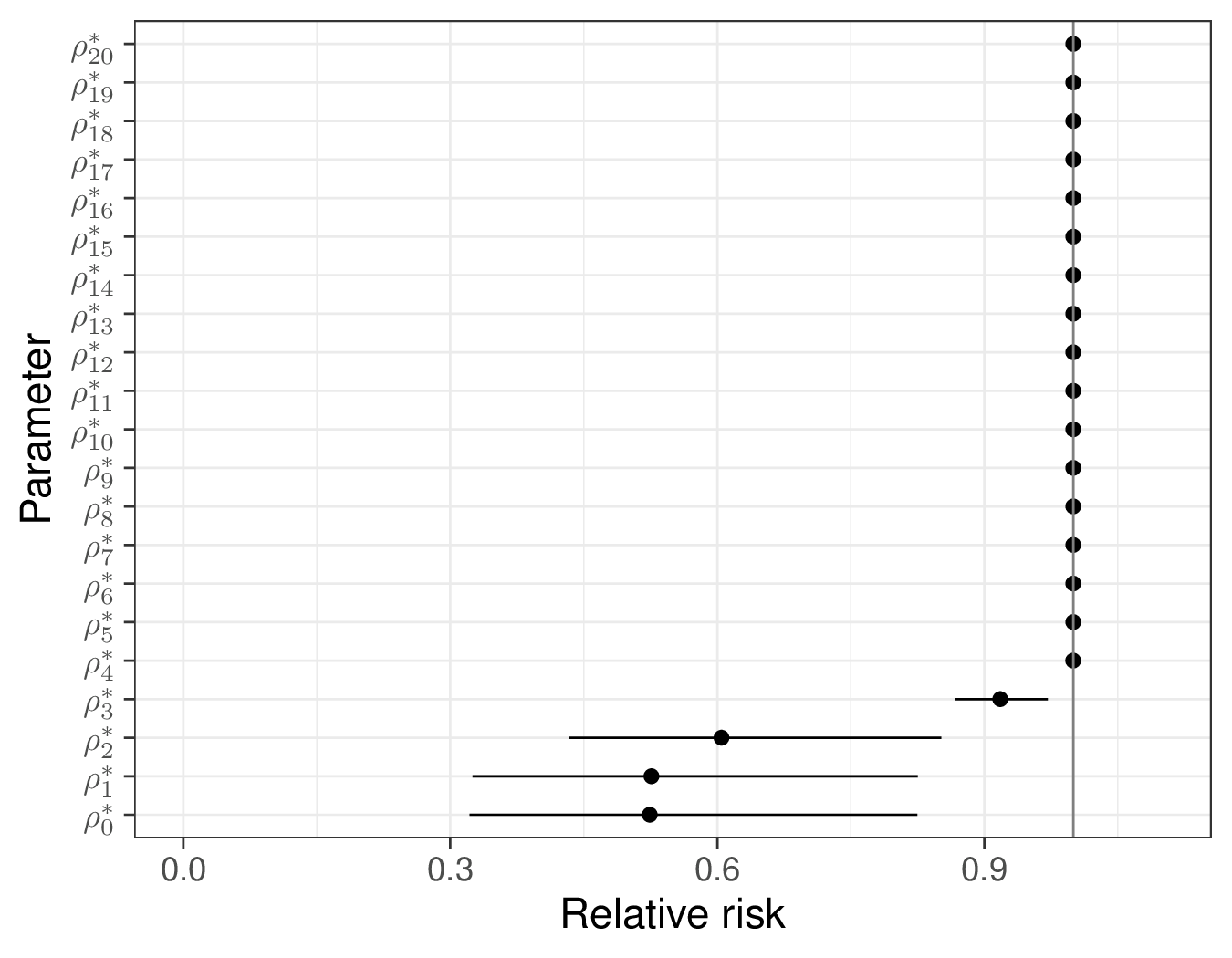
In this case, the model is very quick to run and convergence does not pose any issues. The summary statistics for the posterior distribution of the RRs are shown in Figure 9.5 (a). The RR at time \(j=0\) (which is identical to the estimate from the evidence synthesis \(\rho\) – cfr. Equation 9.7) is estimated to be 0.524 with a 95% interval of \([0.322; 0.825]\), indicating a substantially beneficial effect of the combination therapy over ZDV only.
(a) \(\rho^*_j\).
(b) \(S(j)=\Pr(\text{treatment effective at time }j)\).
Figure 9.5: Posterior distribution summaries for selected nodes.
As time passes, this quickly decreases: at year \(j=3\), the RR is estimated as 0.918 (with a 95% interval of \([0.867; 0.972]\)) and then it goes to 1, indicating that, by then, the treatment is no longer effective and thus produces no benefits.
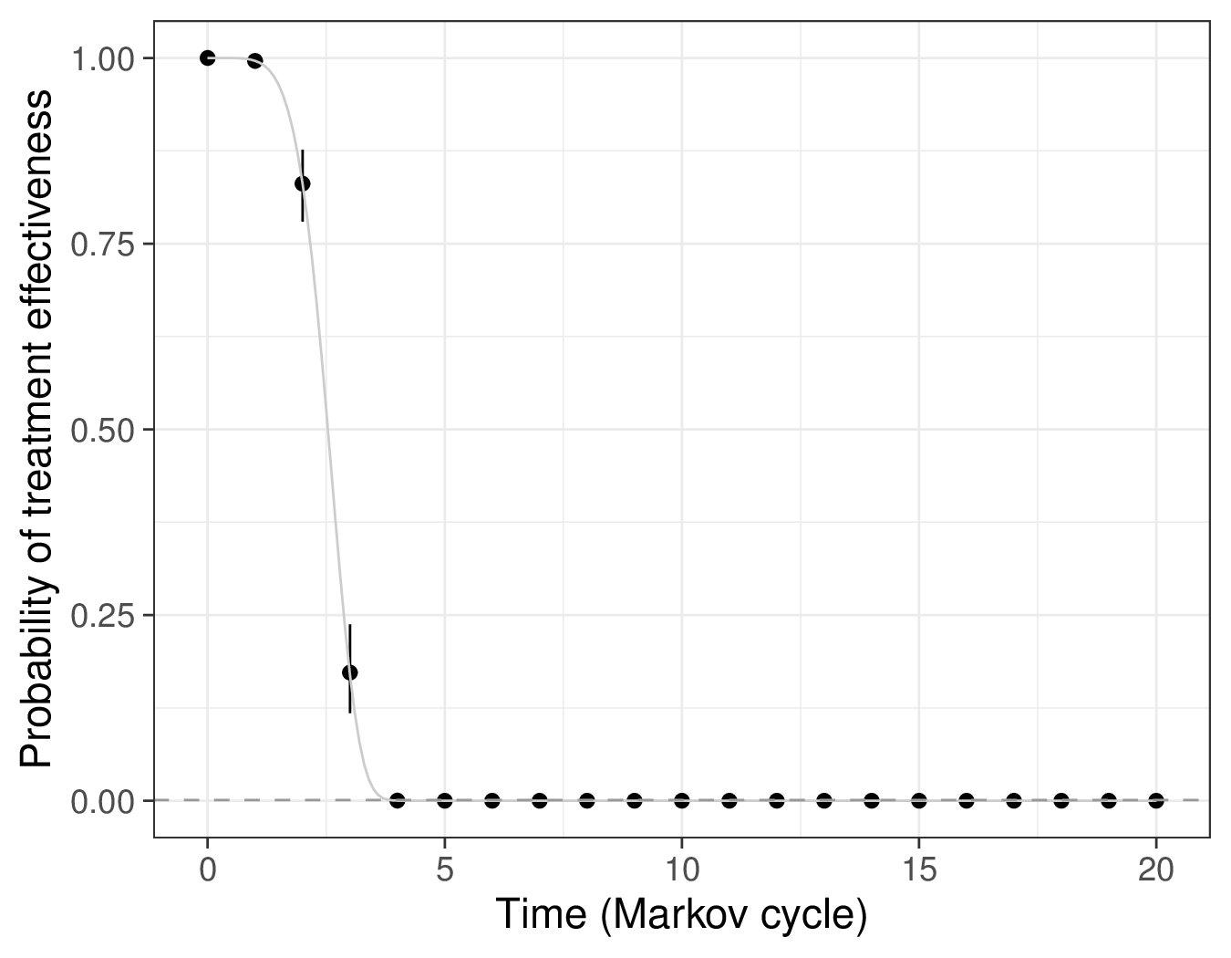
This is consistent with the graph in Figure 9.5 (b), which is based on the posterior summaries for the survival curves induced by the Binomial model for the pseudo-counts \(r_i\). Here, initially, the treatment effectiveness is almost identical to 1 (this holds for years \(j=0,1,2\)), in line with the assumptions in Chancellor et al. (1997). After that, the treatment effectiveness starts to decrease sharply and by year \(j=4\) it is effectively below the threshold eps (indicated by the horizontal dashed line).
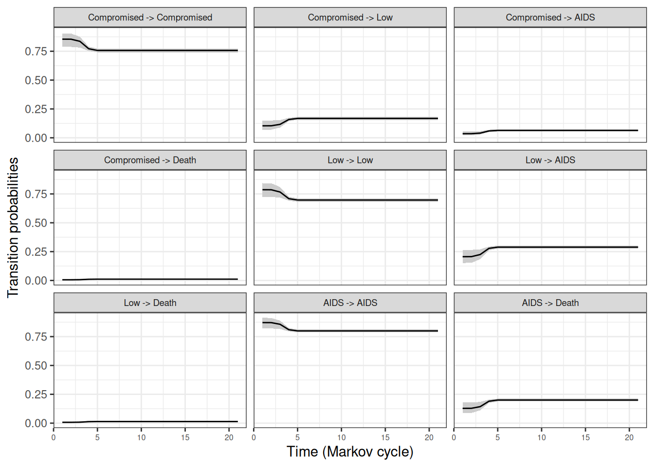
Figure 9.6: Estimates for the posterior distribution of the transition probabilities in the combination therapy arm. These are obtained by applying the time-varying RR to the estimates for the transition probabilities in the ZDV arm. Inititally, the treatment is estimated to be effective and thus there is a reduction in the probability of the progressions; over time, the treatment effect wanes out and the probabilities switch back to the same levels as in the mono-therapy arm.
We can also post-process the simulations from the posterior distributions to construct Figure 9.6, which depicts the probabilities for the possible transitions, in the 3TC+ZDV arm. We present here the mean (dark curve) and the 95% interval (the grey ribbon), across the \(J=20\) years of virtual follow-up for the Markov model.
As long as the treatment is effective, the combination arm shows benefits in decreasing the progressions (from \(s=1\) to \(s'=2,3,4\); from \(s=2\) to \(s'=3,4\) and from \(s=3\) to \(s'=4\)). Once the treatment effect wanes down to 0 (around year 5), then the transition probabilities stops varying over time and revert to the same value as the ZDV arm.
9.2.3 Running the Markov model
Once we have obtained the estimates for the relevant posterior distributions, we need to post-process the results and apply the matrix algebra in order to run the Markov model. The real complexity in this case is that we need to apply the matrix algebra of Equation 9.2 or Equation 9.3 for each MCMC simulations for the model parameters (i.e. the number n.sims, in this case set at 2000).
In order to do so, it is often useful to consider R “arrays”, which are multi-dimensional extensions to simpler matrices. For example, we may need to create an array lambda, with dimension \(n_{\text{\textit{sims}}}\times (J+1) \times S \times S\), in which, for each MCMC simulation \(i=1,\ldots,n_{\text{\textit{sims}}}\) and for each Markov cycle \(j=0,\ldots,J\), we store a \(S\times S\) transition matrix.
Note Indexing vectors and times
Notice the slight inconsistency between the pure mathematical notation and the computer one used in the rest of the chapter. As mentioned above, we consider here Markov cycles \(j=0,\ldots,J\).
However, R does not allow to define a vector using the index 0 and thus in the code below we use j=1,\(\ldots\),J+1 instead, where the index j=1 indicates time \(j=0\), the index j=2 indicates time \(j=1\) and so on.
We demonstrate how to “wrangle” the results from the JAGS model in Example 9.4.
Example 9.4. HIV (continued): Markov model and economic evaluation. We start the post-processing by defining the number of Markov cycles (\(J=20\), in this case, in line with the original analysis of Chancellor et al., 1997) and then a vector start, in which we set up the initial conditions in terms of states occupancy. Often, we assume that all the “virtual cohort” starts in one state, in this case “Compromised CD4”, but we could distribute the individuals across the states, already at time \(j=0\). In this case, we consider a virtual cohort of 1000 individuals (but, again, we could choose any number we like).
Next, we initialise the \(n_{\text{\textit{sims}}}\times (J+1) \times S\) arrays m1 and m2, in which we will store the occupancy matrices. These have three dimensions – the first one indicates the MCMC simulations for the model parameters, the second one the number of the Markov cycles (as mentioned above, we consider from \(j=0\) to \(j=J=20\), i.e. a total of \(J+1\) time points) and the third one indicates the \(S\) states characterising the Markov model. In this case, we set up the arrays to 0, but this is also not essential and, for instance, we could create and fill them with NAs.
In R we can use the function array() to create a multidimensional array – note in the code below that we also use the optional argument dimnames to pass a list of names for each of the three dimensions. This is not essential, but it does help to navigate the objects we are creating and thus we recommend doing so.
Finally, for each MCMC simulation, we initialise the first row of the arrays m1 and m2 to the starting position – this means that at time \(j=0\) every individual is in the state “Compromised CD4”.
# Time horizon for the Markov modelJ=20# Virtual cohort: everyone starts in State Astart=c(1000,0,0,0)# Initialises the array for the number of individuals in each statem1=m2=array(0,c(hiv$BUGSoutput$n.sims,(J+1),S),dimnames=list(1:hiv$BUGSoutput$n.sims,paste0("j=",0:J),states))for (s in1:S){ m1[,1,s]=start[s] m2[,1,s]=start[s]}# Visualises the 'm1' array for the first MCMC simulation (first few rows)m1[1,,] |>head()
At this point, we can use the MCMC simulations for \(\boldsymbol{\lambda}_s\) and \(\rho^*_j\) to construct the actual transition matrices for the two treatment arms, which we indicate as \(\boldsymbol\Lambda^{(1)}\) and \(\boldsymbol\Lambda^{(2)}_j\), for the ZDV and the 3TC+ZDV arm, respectively. In line with the assumptions specified in Example 9.2, the former does not vary with the Markov cycle, while the latter does (and hence is indexed by \(j\)).
We first extract the simulations for the node lambda from the JAGS object hiv into the variable lambda1, which represents the transition matrix for the ZDV arm, \(\boldsymbol\Lambda^{(1)}\). Then, we define a new array lambda2. This is temporarily filled with 0s and we specify its size to be the same as for lambda1, but with an additional fourth dimension, to account for the fact that this will vary with the Markov cycle \(j\).
Once this is done, we can loop over the MCMC simulations i and the Markov cycles j to apply the estimated time-varying RR rho.star[i,j] to the ZDV transitions – for numerical stability and in line with the discussion in Section 9.2.2, we do this using Equation 9.11, which also ensures that each row must sum to 1:
# Formats the simulations for the transition probabilities in matrix formatlambda1=hiv$BUGSoutput$sims.list$lambdalambda2=array(0,dim=c(dim(lambda1),(J+1)))# Makes time-varying transition matrix for combination therapyfor (i in1:hiv$BUGSoutput$n.sims) {for (j in1:(J+1)) {# Applies the time-specific RR to the transition probabilities for the ZDV arm# NB: for numerical stability works on logit(lambda) + log(RR) + adjustment and # then applies the inverse logit transformation to go back to [0-1] scale lambda2[i,,,j]=bmhe::ilogit( bmhe::logit(lambda1[i,,]) +log(hiv$BUGSoutput$sims.list$rho.star[i,j]) +log(1-lambda1[i,,]) -log(1-lambda1[i,,]*(1-hiv$BUGSoutput$sims.list$rho.star[i,j])) )# Rescales the diagonal of the transition matrix, so that each row sums to 1diag(lambda2[i,,,j])=diag(lambda2[i,,,j]) + (1-rowSums(lambda2[i,,,j]))# Ensures that Death is an absorbing state lambda2[i,S,S,j]=1 }}
— this code makes use of the bmhe functions logit() and ilogit() that compute the logit and inverse logit transformations, respectively.
Note Sense-checking the transition probabilities
Once the array lambda2 is computed, we can check that all the entries behave using code like the following.
which(lambda2<0,arr.ind=TRUE)
dim1 dim2 dim3 dim4
Here, we are checking for negative transition probabilities – note that adding the option add.ind=TRUE will explicitly print the indices for all the array dimensions in which the condition we specify is encountered.
Luckily, in our problem there are no such cases – hence the output for dim1 dim2 dim3 dim4 (indicating respectively the MCMC simulations, row, column and time point in the transition matrices), is empty. This broadly suggests that the data used to obtained the pooled RR estimate are reasonably consistent with those observed to obtain the estimates for \(\boldsymbol\Lambda^{(1)}\).
Nonetheless, this type of check is actually very helpful and we recommend embedding it in the workflow, because in case there were unacceptable estimates, we may need to “fix” the resulting transition probabilities.
At this point, we can apply the R version of Equation 9.3 and fill the arrays m1 and m2 with the number of individuals that at each time point visit each of the states, for each MCMC simulation of the model parameters. We can do this compactly (and efficiently) using the R matrix multiplication operator %*%.
for (i in1:hiv$BUGSoutput$n.sims) {for (j in2:(J+1)) { m1[i,j,]=m1[i,j-1,] %*% lambda1[i,,] m2[i,j,]=m2[i,j-1,] %*% lambda2[i,,,j-1] }}# Visualises the two array for the first MCMC simulation (first few rows)cbind(m1[1,,],m2[1,,]) |>head() |>round(2)
As is possible to see from the output of the above R code, now the two arrays have been filled with numeric values for all the time points. Here, we bind the columns for m1 to those of m2. The right-most four columns of the output above show the number of people transiting in each of the four states in the combination therapy, in correspondence of the first MCMC simulation of the model parameters – as is possible to see, more people tend to remain in the less severe state and fewer die.
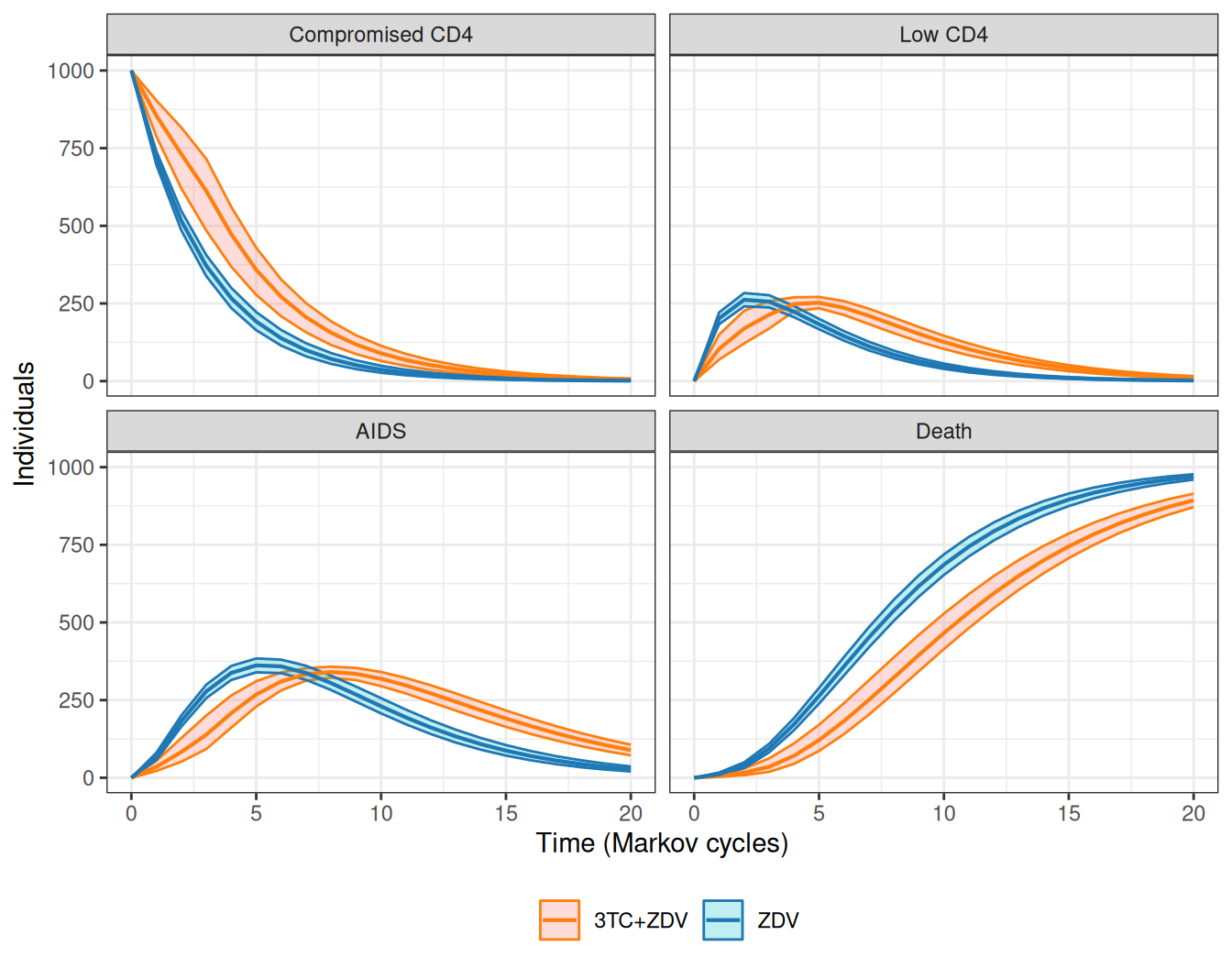
The Markov model simulations can be visualised over the \(J+1\) time points used, in what is often termed as the “Markov trace”. We show the results for the HIV model in Figure 9.7. Over time, the combination therapy consistently maintains a higher number of individuals in the less severe state (“Compromised CD4”) and, crucially, reduces the number of people who die.
Initially, the benefits extend to the other two states too, although at about time \(j=6\), more people remain in the combination than in the mono-therapy arm – this is because at that stage, most people have transitioned out of the “Compromised CD4” state and in the 3TC+ZDV arm fewer people die (and hence more remain in the either “Low CD4” or “AIDS”).
Figure 9.7: Number of individuals in each of the four states, for the two treatment arms.
In Chancellor et al. (1997), the cost-effectiveness analysis is based on life-years gained, meaning that each health state is implicitly assigned a utility value of 1. Again, a more “modern” analysis would focus on utility values associated with each of the states and then QALYs, but here we replicate the original framework, for simplicity.
We can easily obtain the occupancy probability arrays (as in Equation 9.2) by simply rescaling the objects m1 and m2 by the number of individuals in the virtual cohort, set at 1000. These are helpful to continue the post-processing of the results, as we show in the following code – note that we use the lapply() function (see Note 2.2 in Example 2.6), which compactly applies a function over a vector or a list, to ensure that the commands are repeated for each MCMC simulation \(i=1,\ldots,n_{\text{\textit{sims}}}\).
# Defines the occupancy probability arrayspi1=m1/1000pi2=m2/1000# Creates objects with "length of stay" in each statelos1=lapply(1:hiv$BUGSoutput$n.sims,function(i) { pi1[i,,] |>apply(2,sum)}) |>bind_rows()los2=lapply(1:hiv$BUGSoutput$n.sims,function(i) { pi2[i,,] |>apply(2,sum)}) |>bind_rows()
We can use these objects to summarise the results and compute the expected length of stay in years for each treatment arm and for each of the \(S\) states of the Markov model, e.g. using the following simple R code.
los1 |> bmhe::stats()
                     mean         sd      2.5%    median     97.5%
Compromised CD4  3.552654 0.13885803  3.293725  3.546791  3.842771
Low CD4          1.701259 0.07116863  1.567184  1.697992  1.850448
AIDS             3.641863 0.14565022  3.368792  3.637752  3.940041
Death           12.104224 0.20971222 11.689237 12.104198 12.511436
los2 |> bmhe::stats()
                    mean         sd     2.5%   median     97.5%
Compromised CD4 5.130759 0.35576101 4.375209 5.151412  5.784945
Low CD4         2.345948 0.08591254 2.186687 2.344993  2.515648
AIDS            4.217945 0.12852951 3.972561 4.216163  4.469564
Death           9.305348 0.38054294 8.620419 9.281497 10.134087
We can see from these summary statistics that the combination therapy tends to have longer expected time in the less severe state and again, consistently with the findings above, shorter expected years in the state “Death”.
We can also produce an estimate for the overall number of years alive (or Life Years Gained, LYG) in the two treatment arm and, by difference, a measure of treatment effectiveness, \(\Delta_e\).
In comparison to Chancellor et al. (1997), our model returns a larger differential in terms of years of life gained – this is because we allow for the treatment effect to wane off beyond the hard cutoff of two years set in the original analysis.
Similar analyses can be performed by combining the occupancy array pi1 and pi2 with the estimated posterior distributions for the various costs. We do this using the following R code, which returns the output in the form of a “tibble” that can be further aggregated to obtain relevant summaries.
# Define discount rated=0.06# ZDV armc1=lapply(1:hiv$BUGSoutput$n.sims,function(i) {# Probability of occupancy with dimension: (J+1) rows x S columns pi1[i,,] |>as.data.frame() |>cbind(# Vector of times and drug costj=0:J,c_drug=rep(2278,(J+1)),# Matrix with cost of community care with dimension: (J+1) x Smatrix(rep(hiv$BUGSoutput$sims.list$c.comm[i,],(J+1)), (J+1),S,byrow=T,dimnames=list(0:J,paste0("c_comm_",states)) ),# Matrix of cost of direct care with dimension: (J+1) x Smatrix(rep(hiv$BUGSoutput$sims.list$c.direct[i,],(J+1)), (J+1),S,byrow=T,dimnames=list(0:J,paste0("c_direct_",states)) ) ) |>as_tibble()}) |>bind_rows() |># Applies discounting to all costsmutate(across(starts_with("c_"),~ .x/(1+d)^j)) |># Computes the cost for each statemutate(`Compromised CD4`=`Compromised CD4`* (`c_drug`+`c_comm_Compromised CD4`+`c_direct_Compromised CD4`),`Low CD4`=`Low CD4`*(`c_drug`+`c_comm_Low CD4`+`c_direct_Low CD4`),`AIDS`=`AIDS`*(`c_drug`+`c_comm_AIDS`+`c_direct_AIDS`),sim=rep(1:hiv$BUGSoutput$n.sims,each=(J+1)) ) |># Selects only the relevant columnsselect(sim,j,`Compromised CD4`,`Low CD4`,`AIDS`)
First, we define the value of the discount rate, \(d\) (see Equation 5.2) – Chancellor et al. (1997) use a value of 6% for costs, although perhaps a more “modern” analysis would apply a smaller rate (see the discussion in Section 5.1).
Then, we start creating an object c1, in which we want to store the costs incurred in each state for each time point and derived by using different MCMC simulations for the model parameters. Firstly, we use again the lapply() function to repeat the commands for each MCMC simulation \(i=1,\ldots,n_{\text{\textit{sims}}}\) and then we build a data frame, including the relevant variables. We start by including the \(i-\)th element of the occupancy probability array pi1, which we augment with a vector j, to keep track of the Markov cycle. Then, we add the various costs: the column c_drug is a vector in which the value 2278 is repeated for J+1 times: this is because the cost of ZDV is fixed for each Markov cycle. Next, we add the cost of community care: the JAGS object outputs a matrix with \(n_{\text{\textit{sims}}}\) rows and \(S\) columns for this variable, which is assumed to not vary over the Markov cycles. Thus, we select the first row of values from the JAGS object hiv and create a matrix with J+1 rows and S columns using the code
Notice, again, the use of the option dimnames to associate meaningful names to the dimensions of the matrix – once more, this is not essential, but it is a helpful sanity check and will facilitate further wrangling of the data, later. The same reasoning applies for the cost of direct care, which are also estimated as a matrix of \(n_{\text{\textit{sims}}}\times S\) simulations in the JAGS model. Finally, for all MCMC simulations, we store the resulting data frame as a tibble, for ease of post-processing. At this stage, c1 is still a list with \(n_{\text{\textit{sims}}}\) elements, each of which looks like the following
(this output is for i=1 and, as such, it only has \(J+1=21\) rows, one for each time point).
Outside the lapply() function, we add the dplyr function bind_rows(), which is used to combine all the 2000 elements of the list into a single tibble. The resulting object has \(n_{\text{\textit{sims}}}\times (J+1)=2000\times 21=42000\) rows.
Next, we apply discounting to all the cost variables. Here, we have made sure to follow a specific naming convention, where all the cost variables are labelled as c_XXX. Thus, we can use the command
mutate(across(starts_with("c_"),~ .x/(1+d)^j))
to compactly apply the discounting formula x/(1+d)^j (cfr. Equation 5.2) to each variable whose name starts with the string "c_".
Finally, we first compute the overall cost associated with each state as the product of the probability of occupancy and the sum of the relevant item costs and then select only the relevant columns, which produces the object of interest, c1, the first few rows of which look like the following.
As for the combination therapy arm, to create another object c2, we can basically copy and paste the code used above, with the two differences that: i) we use the occupancy probability array pi2 (instead of pi1); and ii) we define the drug costs as c_drug=cbind(hiv$BUGSoutput$sims.list$c.comb[i,]) because, in this case, the cost of acquisition of the drug does vary with the Markov cycles and thus, for each MCMC simulation, we obtain a vector of J+1 values, which we add as a column to the data frame using the R built-in function cbind().
Once these tibbles are available, we can wrangle them further to produce any relevant summary or to build a graph using ggplot2. For instance, we can use the following R code to derive summary statistics for the total cost by states across all years.
                    mean       sd      2.5%   median    97.5%
Compromised CD4 30489.95 2498.667 25757.553 30452.23 35424.60
Low CD4         11533.33 1210.854  9432.975 11459.96 14037.24
AIDS            34435.75 3218.337 28370.284 34351.82 41211.68
Similarly, we can summarise the total costs across both states and years as well as the incremental value for the combination therapy, \(\Delta_c\), using the following R code.
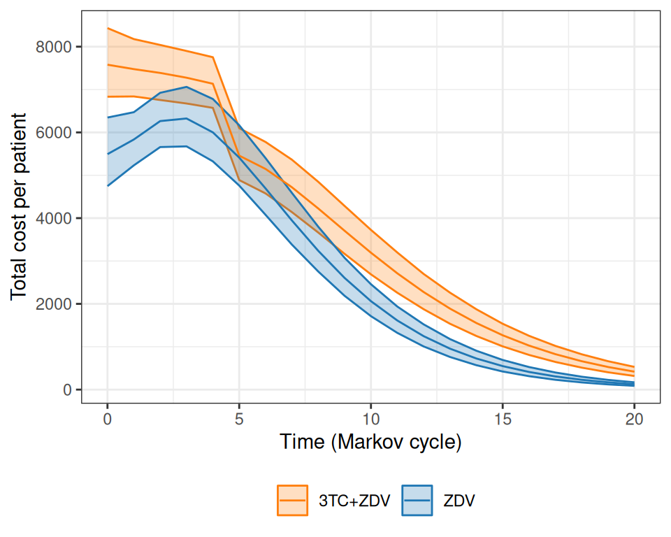
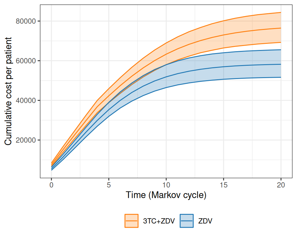
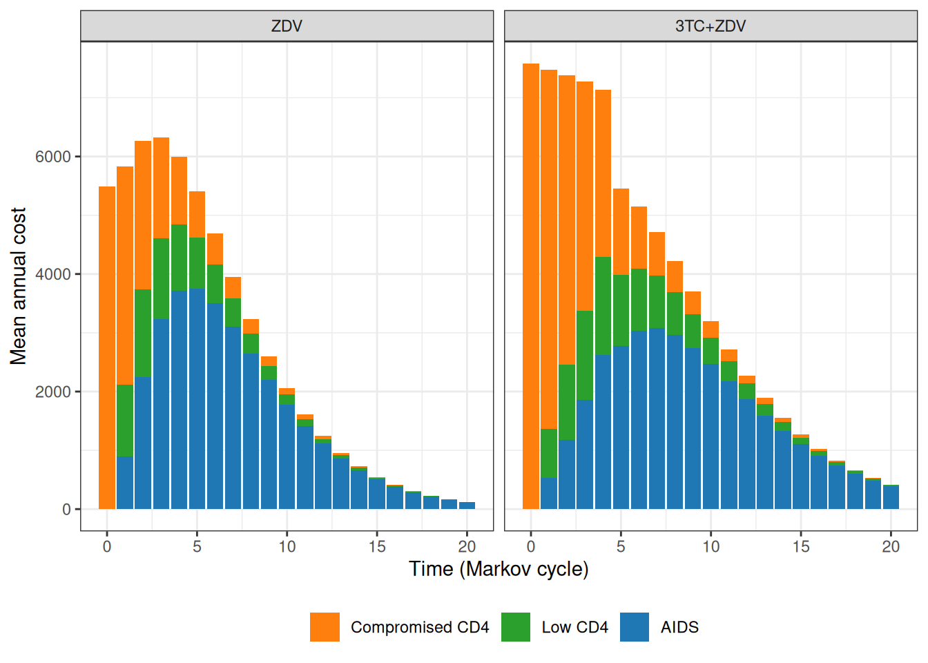
Figure 9.8 shows the progression of the total cost per patient over the course of the virtual follow-up.
(a)
(b)
(c)
Figure 9.8: Analysis of the total costs over the course of the virtual follow-up. Panel (a) shows the estimated total cost per patient over the time of the Markov simulation, while panel (b) depicts the overall cumulative costs over time, for the two treatment arms. Panel (c) shows a barplot with the contribution of each state to the yearly costs in the two treatment arms.
As is possible to see in Figure 9.8 (a), while at the beginning the combination therapy is more expensive, the two curves tend to get closer and closer. The combination therapy is still more expensive, but much less so and, interestingly, the interval estimates are on top of each other. Figure 9.8 (b) shows the progression of the overall cumulative costs, which highlights the fact that the combination therapy does accrue larger costs by the end of the virtual follow-up. Finally, Figure 9.8 (c) shows how annual costs are split, on average, across the states, indicating again that the combination therapy has higher costs mostly for the less severe states, especially for the first few years of the Markov model simulation.
In comparison to Chancellor et al. (1997), the costs are substantially higher, because we assume a larger cost for direct medical care (to account for the uncertainty in the hospital data, including the values observed in the alternative source). In addition, the full cost of the combination therapy generally occurs for longer periods (more or less up to \(j=4\)), while the base-case analysis in the original model assumes that after two years the combination therapy reverts to mono-therapy with no uncertainty whatsoever.
9.3 Three-state Markov model
Another case in which Markov models are particularly popular in HTA is to evaluate a specific disease history, typically related to cancer and often referred to as “Three-state Markov model”.
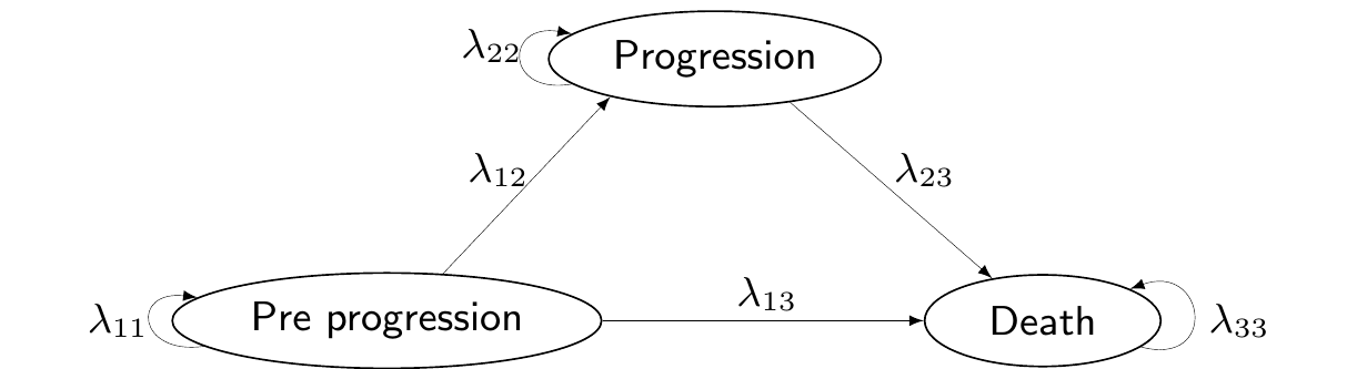
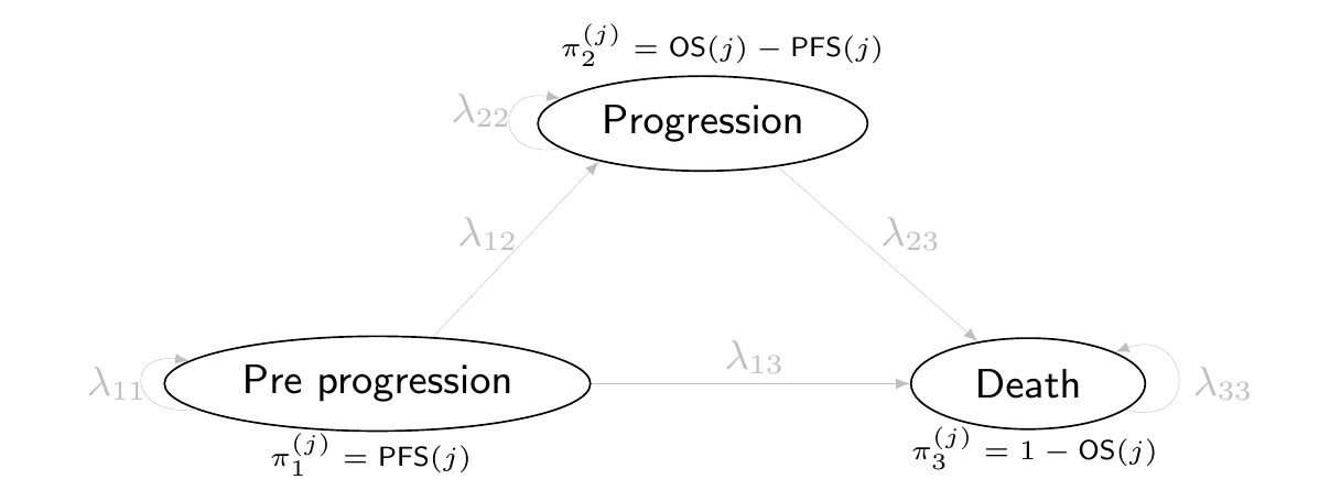
In this specific setup, the relevant population is made by individuals who are in the state of “Pre progression”, i.e. they have already been diagnosed with cancer. In future times, their condition may deteriorate further in two ways: either they move into a state of “Progression” (e.g. through metastases or a general worsening of the cancer), or to the absorbing state of “Death”. From “Progression”, the clinical representation of the disease does not allow individuals to revert to a less severe state and the only available move is towards “Death”. Figure 9.9 shows this natural history of the disease, graphically.
Figure 9.9: A graphical representation of the “Three-state cancer Markov model”.
While it may look like a rough simplification, this structure is often suitable to describe the life-course of cancer patients, especially for aggressive tumours, where, effectively, there is no cure and thus it is not possible to reverse to less severe states of the illness.
When dealing with these situations, we often link the output of a survival analysis (as presented throughout Chapter 8) to the Markov model machinery. We showcase two ways of doing this, depending on the nature of the available data.
9.3.1 Three-state Markov models with individual-level data
As mentioned in Section 8.3.2, ideally, we have access to individual-level data (e.g. from a randomised trial), describing the “event history” for each patient. Table 9.4 shows an example of this sort of data – in fact this is the same dataset considered in Example 8.1.
Table 9.4: A snippet of the data included in the TA 174. Source: Williams et al. (2017b)
Patient
Treatment
Progression?
Death?
Progression time
Death time
1
RFC
1
0
31.99
32
2
RFC
1
0
30.55
30.6
\(\ldots\)
\(\ldots\)
\(\ldots\)
\(\ldots\)
\(\ldots\)
\(\ldots\)
9
FC
1
0
35.73
36
10
RFC
1
1
0.17
0.46
\(\ldots\)
\(\ldots\)
\(\ldots\)
\(\ldots\)
\(\ldots\)
\(\ldots\)
NoteDigitising well is hard work (and comes with assumptions)…
As mentioned in Note 8.2 in Example 8.1, the data are obtained through digitisation and substantial post-processing to recreate all the individual trajectories in terms of all the relevant transitions – from pre-progression to progression; from pre-progression to death; and from progression to death.
The death times generated for patients who had a corresponding progression time matched closely the event times from the scanned pre-progression curve. This works if we assume a “semi-Markov”/clock-reset approach for the transition from progression to death. With this terminology, we indicate the assumption that continuous transitions rates can also depend on the time spent in the current state. This relaxes the more stringent Markov(1) assumption (see Equation 2.11), under which the transitions are “memory-less” and all that matters to determine the next state is the current one and not the full history (see also the discussion in Thom et al., 2025b, sec. 9.3.3).
In the case of the NICE TA174 synthetic data generated by Williams et al. (2017a), the semi-Markov assumption is fundamental because it lets the risk of moving to the next health state depend not only on the current state (e.g. progressed) but also on how long a patient has been in that state. In other words, the clock resets at progression and time since progression, not the total time since baseline, governs the hazard of death.
This flexibility is crucial when reconstructing synthetic individual-level data from digitised survival curves. If we assumed a strict Markov(1) process, the transition from progression to death could only depend on being in the progressed state, ignoring for how long each individual had sojourned there. This, in turn, would make it impossible to align reconstructed death times with the observed post-progression survival pattern, because the real data show that the risk of death changes with time since progression.
By using a semi-Markov model, we can model the post-progression hazard separately directly from the digitised post-progression survival curve, without having to match every progression event exactly to an individual’s pre-progression time. The clock-reset assumption lets us treat the progression to death process independently, which greatly simplifies reconstruction while remaining realistic.
Ultimately, under a pure Markov(1) assumption, it may be near-impossible to generate individual-level data with event times for each patient, because of the lack of the complete history. Relaxing this to a semi-Markov approach does offer more possibilities, especially if we can complement the limited information from the survival curves with additional evidence.
This type of data would allow us to estimate directly all the relevant transition probabilities, because they contain information about the complete history of each individual and so we can use them to construct the “risk set” for each possible transition and then estimate the time-to-event.
Specifically, once the survival curves are estimated for each of the relevant subsets, we can provide estimates of the transition probabilities from a state \(s\) to another state \(s'\) at time \(j\), using the survival curve computed for two consecutive times \(j\) and \(j+\delta_j\) (where \(\delta_j\) constitutes the length of the Markov cycle) as \[
\lambda_{jss'} \approx 1 - \frac{S(j+\delta_j)}{S(j)}.
\tag{9.12}\] This is because the ratio \(\frac{S(j+\delta_j)}{S(j)}\) indicates the proportion of individuals who still have not experienced the event of interest (either progression or death) at time \(j+\delta_j\), out of those individuals who were still at risk at the beginning of the interval \([j;j+\delta_j]\). Thus, the complement to 1 represents the proportion of individuals who between times \(j\) and \(j+\delta_j\) have indeed experienced the event of interest.
If the Markov cycle is too wide, then the approximation based on the survival curve is very coarse and possibly quite biased in comparison to the underlying, continuous transition probability \(\lambda_{jss'}\) for any given time \(j\). But if the width of the interval is reasonably small, then Equation 9.12 is an acceptable discrete approximation of the continuous value – of course, what is “reasonably small” depends on the context.
If we have the full history of all the individuals, we can subset the data to derive the relevant risk sets (see in details the computations in Example 9.5):
Subset 1: individuals at risk of making the transition from “Pre-progression” to “Progression”
Subset 2: individuals at risk of dying from “Pro-progression” (without first transiting in “Progression”)
Subset 3: individuals at risk of dying from “Progression”.
We can use these data to perform the survival analysis and apply Equation 9.12 to directly estimate \(\lambda_{j12}\), from Subset 1; \(\lambda_{j13}\), from Subset 2; and \(\lambda_{j23}\), from Subset 3.
Moreover, using the fact that the transitions are mutually exclusive and exhaustive, we can estimate indirectly\[
\begin{aligned}
\lambda_{11j} & =1-\lambda_{12j}-\lambda_{13j} \\
\lambda_{22j}& =1-\lambda_{23j}.
\end{aligned}
\] and thus, since “Death” is an absorbing state, we can complete the transition matrix \[
\boldsymbol\Lambda_j = \left(\begin{array}{ccc} \lambda_{j11} & \lambda_{j12} & \lambda_{j13} \\ 0 & \lambda_{j22} & \lambda_{j23} \\ 0 & 0 & 1 \end{array}\right).
\] Once the transition matrix is obtained for each relevant time period (Markov cycle), we can simply run the Markov model of Figure 9.9 to derive all the relevant outputs.
Example 9.5. NICE TA174 (adapted and expanded from Williams et al., 2017b): three-state modelling. We consider again the data for NICE TA174; in particular, we can target the two underlying events (progression and death). The analysis based on the time until a progression is observed determines the so-called “progression-free survival” (PFS), while the analysis targeting death as the event of interest determines the so-called “overall survival” (OS) – see the discussion in Section 8.3.2.
It is possible to use the survHE function make_data_multi_state() to wrangle the original dataset and create the relevant indicator to then define the “risk sets”.
# Uses survHE to restructure the datasetrisk_set=survHE::make_data_multi_state(data)# Shows the first few rows of the resulting dataset. Here, treat=1 is RFCrisk_set |>as.data.frame() |>head() |>print(digits=2)
The object risk_set contains the information in Table 9.4, but restructured to account for the possible transitions. These are described in the columns labelled from and to (or, more compactly, in the column labelled trans); for instance, the first row of the dataset describes the time necessary for the patient indexed by the patid 1 to move from “Pre-progression” to “Progression, which happens in 32 time units (e.g. months).
The variables Tstart and Tstop indicate the times at which the individual enters and exits the relevant risk set – in other words, the individual associated with patid=1 is at risk of making the transition from “Pre-progression” to “Progression” immediately at enrollement (as is reasonable) and until the event actually happens.
The dataset also contains progression and death indicators, respectively in the variables prog and death, taking values 0 or 1 if that specific event is censored or fully observed. Finally, the progression and death times are also recorded separately in the variables prog_t and death_t.
We can filter the dataset to select specific cases and sub-risk sets, as shown in the following R code. For instance, filtering for trans==1 selects all the individuals who are at risk of making the transition from “Pre-progression” to “Progression”. In fact, there are different outcomes observed among them; for instance, the combination trans==1,prog==0,death==0 returns the subset of patients who while in “Pre-progression” have been fully censored, i.e. those for whom we do not know the actual time to progression or to death. In this case, the reported data indicate the time of censoring.
# Selects patients in Pre-progression who are fully censoredrisk_set |> dplyr::filter(trans==1,prog==0,death==0) |>slice(1:3) |>as.data.frame() |>head() |>print(digits=2)
   id from to trans Tstart Tstop  time status treat prog death prog_t death_t
1 249    1  2     1      0 0.058 0.058      0     1    0     0  0.058   0.058
2 250    1  2     1      0 3.797 3.797      0     1    0     0  3.797   3.797
3 251    1  2     1      0 5.466 5.466      0     1    0     0  5.466   5.466
Another subgroup is made by those who have died before progression by filtering trans==1,prog==0,death==1. Notice that, in this case, the indicator prog is set to 0 to indicate that these patients are censored, with respect to the event of interest (progression).
# Selects patients in Pre-progression who die before progressionrisk_set |> dplyr::filter(trans==1,prog==0,death==1) |>slice(1:3) |>as.data.frame() |>head() |>print(digits=2)
   id from to trans Tstart Tstop time status treat prog death prog_t death_t
1 527    1  2     1      0   1.5  1.5      0     1    0     1    1.5     1.5
2 528    1  2     1      0   2.1  2.1      0     1    0     1    2.1     2.1
3 529    1  2     1      0   2.6  2.6      0     1    0     1    2.6     2.6
Similar reasoning and code allow us to select different subgroups for the other transitions. For instance, the code
# Selects patients in Pre-progression who move to Progression and haven't diedrisk_set |> dplyr::filter(trans==2,prog==1,death==0) |>slice(1:3) |>as.data.frame() |>head() |>print(digits=2)
  id from to trans Tstart Tstop time status treat prog death prog_t death_t
1  1    1  3     2      0    32   32      0     1    1     0     32      32
2  2    1  3     2      0    31   31      0     1    1     0     31      31
3  3    1  3     2      0    28   28      0     1    1     0     28      28
retrieves the patients at risk of dying from “Pre-progression”, who have progressed but have not been observed to die. For these individuals, Tstop identifies the time at which they have reached the state “Progression” and the indicator for death is set to 0, as they are censored to the main event for the underlying transition (“Pre-progression” to “Death”). This is confirmed by the fact that the indicator status is set to 0 for these patients.
We can use the three relevant risk sets identified by the full subsetting based on trans==1 (“Pre-progression” to “Progression”), or trans==2 (“Pre-progression” to “Death”), or trans==3 (“Progression” to “Death”) and fit suitable survival models, for example as in the following R code and using survHE (see Section 8.4).
# Sets up informative priors on the Gompertz parameters to stabilise inferencepriors=list(gom=list(a_alpha=1.5,b_alpha=1.5))# Runs survival models on the specific subsets to obtain estimate # of the various transition probabilitiesm_12=fit.models(Surv(time,status)~as.factor(treat),data=risk_set |> dplyr::filter(trans==1),distr="gom",method="hmc",priors=priors)m_13=fit.models(Surv(time,status)~as.factor(treat),data=risk_set |> dplyr::filter(trans==2),distr="gom",method="hmc",priors=priors)m_23=fit.models(Surv(time,status)~as.factor(treat),data=risk_set |> dplyr::filter(trans==3),distr="gom",method="hmc",priors=priors)
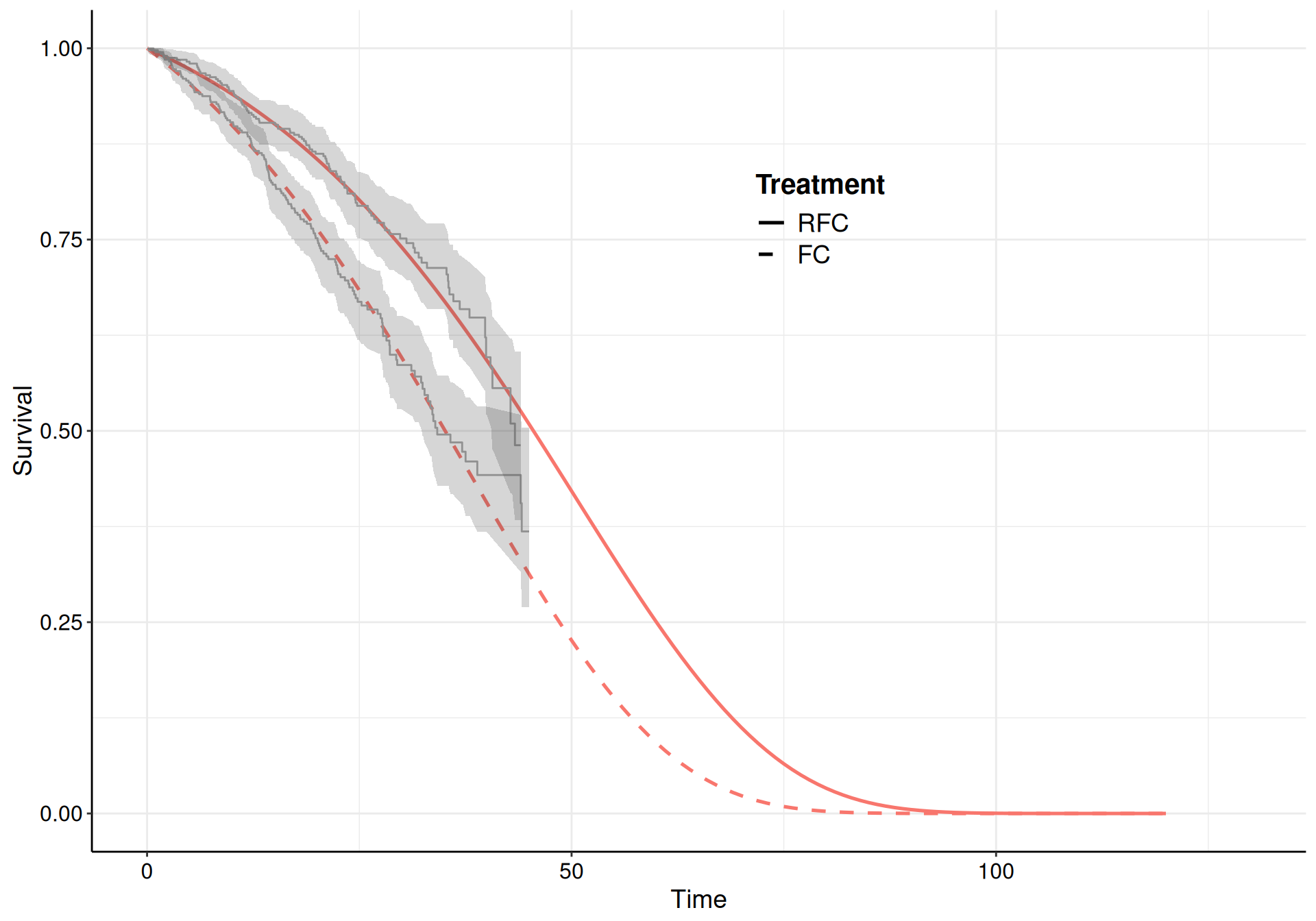
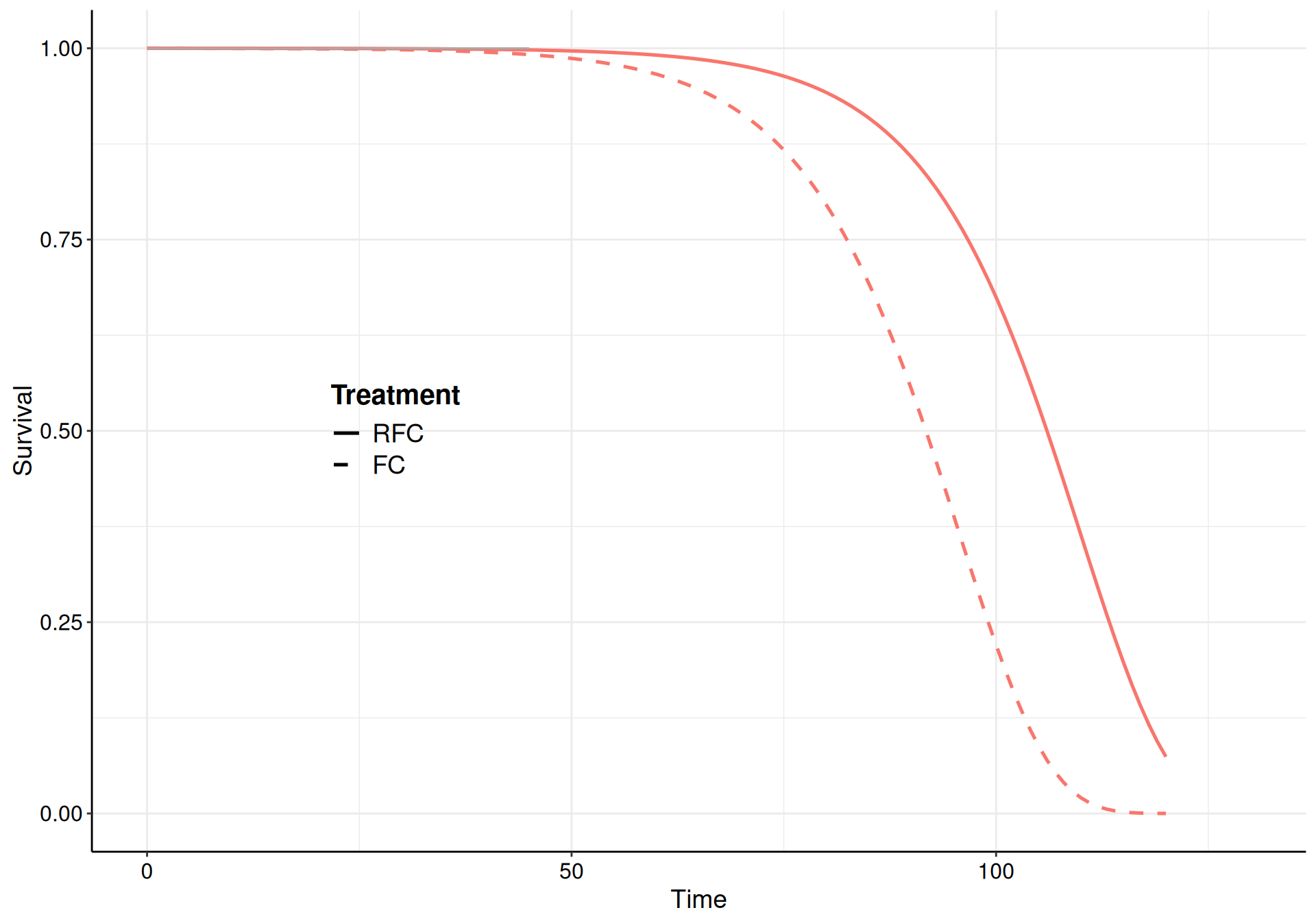
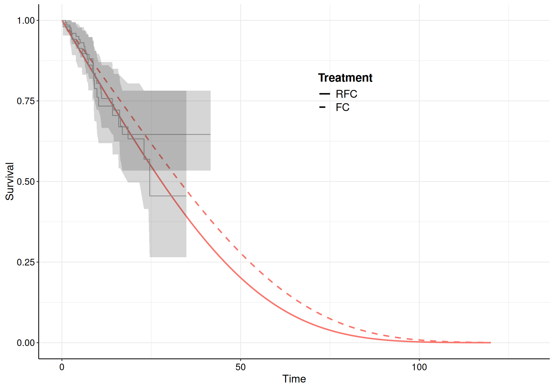
Here, we choose a Gompertz model for all the transitions and specify informative priors to guard against the sparse information present in some of the risk sets (specifically for the transition from “Pre-progression” to “Death”, which is characterised by large censoring – see Figure 9.10 (b)).
(a) Pre-progression to progression.
(b) Pre-progression to death.
(c) Progression to death.
Figure 9.10: The survival curves estimated using a Gompertz model for the three subsets of the NICE TA174 data.
While the model fit to the observed data is reasonably good for all three, the extrapolation to 120 months is not great for the “Pre-progression” to “Death” transition, where the curves barely reach median time. As mentioned above, this is due to the large amount of censoring (as evidenced from the KM curves in Figure 9.10).
We can use the survHE function three_state_mm(), which takes as inputs three model fit objects (such as m_12, m_13 and m_23) obtained in the format of survHE::fit.models() and post-process the estimates to create a tibble with the progression of individuals over the three states. For instance, the command
produces an object mm, which contains the resulting simulations in the tibble mm$m.
# A tibble: 242,000 × 11
   profile  time `Pre-progressed` Progressed    Death sim_idx lambda_11 lambda_12
   <chr>   <dbl>            <dbl>      <dbl>    <dbl>   <int>     <dbl>     <dbl>
 1 FC          0            1000        0    0              1     1       0
 2 FC          1             991.       8.89 0.000781       1     0.991   0.00889
 3 FC          2             982.      17.9  0.0936         1     0.991   0.00921
 4 FC          3             973.      27.1  0.286          1     0.990   0.00955
 5 FC          4             963.      36.4  0.585          1     0.990   0.00989
 6 FC          5             953.      45.9  0.998          1     0.990   0.0103
 7 FC          6             943.      55.5  1.54           1     0.989   0.0106
 8 FC          7             933.      65.2  2.20           1     0.989   0.0110
 9 FC          8             922.      75.0  3.01           1     0.989   0.0114
10 FC          9             911.      85.0  3.97           1     0.988   0.0118
# ℹ 241,990 more rows
# ℹ 3 more variables: lambda_13 <dbl>, lambda_22 <dbl>, lambda_23 <dbl>
Here, we have used nsim=1000 simulations – in other words, for each simulated values from the posterior distribution of the transition probabilities \(\boldsymbol\lambda\), we run the algebra to construct a version of the Markov model, in terms of how many people transit from each of the states at each given time points in the time horizon (from 0 to 120 months). To run the 1000 simulations, the model takes about 5 minutes – in comparison to the case shown in Example 9.4, this is much longer because, in the current model, the time horizon (120 months) is 10 times as long.
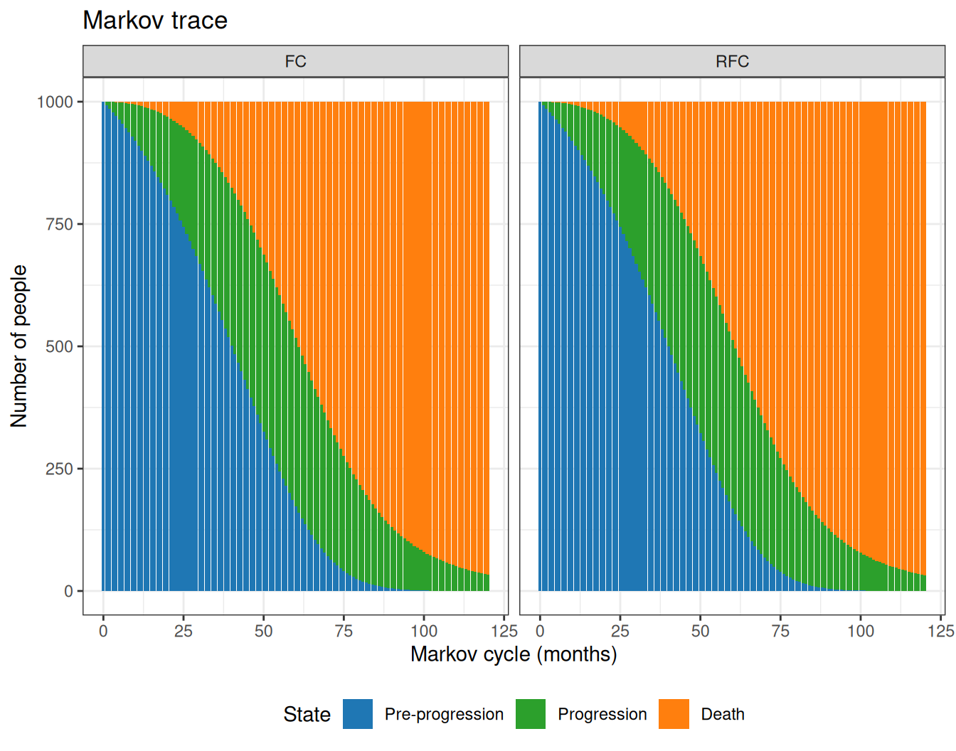
Figure 9.11 shows the Markov trace computed using the mean estimates for the state occupancy at different cycles. As is possible to see, the active treatment (RCF) seems to keep more patients for longer in the “Pre-progression” state, thus reducing the overall number of people who end up in the “Death” states, towards the end of the time horizon.
Figure 9.11: The Markov trace for the analysis of the NICE TA174.
We can also post-process the simulation results further to obtain a measure of “gain” in terms of the average time spent alive (and thus some measure of Life Years Gained) from the two treatments, for instance using the following R code.
# A tibble: 2 × 5
  profile  mean    sd `2.5%` `97.5%`
  <chr>   <dbl> <dbl>  <dbl>   <dbl>
1 FC       5.07 0.732   4.01    6.66
2 RFC      5.41 0.664   4.38    6.93
As is possible to see, the RFC arm shows some gains over the FC arm, which confirms the visual inspection of Figure 9.11. Using the nsim=1000 simulations, we can obtain a measure of uncertainty around this central estimate too.
9.3.2 Partition survival modelling
In cases where the full even history for each individual is not available, we need to resort to alternative methods in order to analyse a three-state cancer model. In these cases, one of the most popular workaround is to use “partitioned survival analysis” modelling (PSM, Woods et al., 2017).
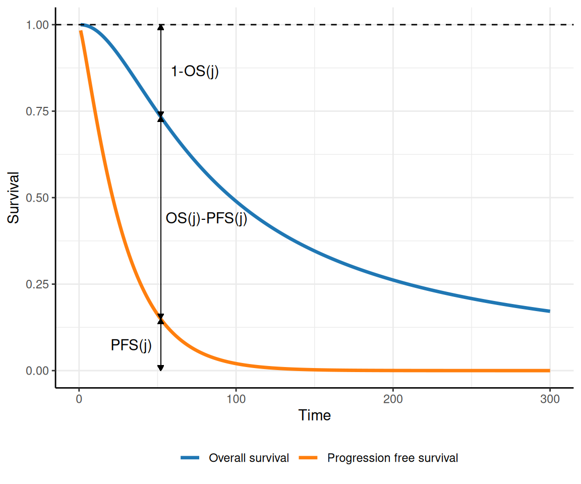
The idea is that although we may not have access to a full dataset describing the times at which transitions occur for each individual, we typically can estimate (perhaps through digiisation from published studies) the survival curves for the main outcomes, OS and PFS. For instance, consider the curves depicted in Figure 9.12: at each time point \(j\) on the \(x\)–axis, we can read off the curves:
the proportion of individuals who are still in pre-progression as the area under the PFS curve (indicated as \(\text{PFS}(j)\), in the figure);
the proportion of individuals who have died as the complement to 1 of the area under the OS curve (indicated as \(1-\text{OS}(j)\), in the figure); and
the proportion of individuals who have moved to progression as the area between the two curves (indicated as \(\text{OS}(j)-\text{PFS}(j)\), in the figure).
Figure 9.12: A graphical representation of the concept of partition survival analysis. Using PFS and OS, we can determine the proportion of individuals who are in each of the three states, at any given time.
Interestingly, this works in the specific circumstances of the three-state cancer Markov model, in which transitions only occur “forward” (i.e. it is not possible to revert to a less serious health state). This is often indicated as cumulative and non-reversible timeline. By definition, \(\text{PFS}(t)\) and \(\text{OS}(t)\) are monotonically decreasing, while backwards transitions would imply an increase in the curves over two consecutive times, which is not supported by the data. Thus, if the underlying disease/natural history suggests that individuals can move back and forth, we need to use different data (e.g. observed transition matrices)
In addition, by necessity, we must assume independence between the two curves, given that we do not observe the full individual history. This is almost invariably a critical point, because in fact, the same individuals generally contribute to both – the same person may have experienced a transition to progression and then die. However, only from the survival curves, there is no way to account for this underlying correlation.
Figure 9.13: The partition survival representation of the three-state Markov model. Here, we cannot estimate the actual transition probabilities \(\boldsymbol\lambda\) (which in fact are greyed out), but only the proportion of individuals that at each time point transit from the three states, \(\boldsymbol\pi\).
One main limitation for PSM is that we cannot estimate the full transition probabilities, from the observed data. We cannot get the transition probabilities – only the occupancy probabilities, as indicated in Figure 9.13. The possible transitions and the relevant probabilities \(\lambda_{ss'}\) are all greyed out, because we cannot directly identify them from the available data – what we can estimate are the proportion of individuals who, at each time period, transit in the three states, \(\pi_{s}^{(j)}\).
Jackson et al. (2025) argue that perhaps the most critical limitation of PSMs is that because of the implied independence between OS and PFS, the necessary extrapolation from the observed curves to cover the longer-term follow for the three-state Markov model is likely to result in important bias.
An archetypical case is when extrapolated PFS probabilities end up being estimated with larger values than the corresponding OS probabilities, implicitly implying that a negative proportion of the cohort is occupying the progressed state. For this reason, Jackson et al. (2025) caution modellers and suggest care is needed in using PSMs uncritically.
9.4 Conclusions
This chapter has presented a detailed description of how multi-state (Markov) models are used in HTA applications. We have concentrated on two typical examples – the first one using a combination of data directly on the relevant transitions across a set of finite and mutually exclusive states, used to describe the “natural history of a disease” of interest. This structure naturally lends to a Bayesian modelling, which is particularly helpful to combine different sources of information into a principled framework to assess fully the underlying uncertainty in the model inputs and the associated one onto the economic outputs.
We have also linked up the use of MMs with survival modelling, in what is often termed a “three-state cancer Markov model”. This is a special case of Markov model, in which transitions are informed by suitable survival models – we have showed the case where individual-level data are available to reconstruct the full event history and the one where we need to resort to simplifying assumptions (that often are harder to meet, in practice), which allow to get a Markov model-like structure, using partition survival modelling.
In the next part of the book, we will concentrate on more advanced problems and modelling frameworks, starting from methods to deal with missing data and then the increasingly important and popular topic of population adjustment and the analysis of the value of information.
Briggs, A, Sculpher, M., Claxton, K., 2006. Decision Modelling for Health Economic Evaluation. Oxford University Press.
Chancellor, J.V., Hill, A.M., Sabin, C.A., Simpson, K.N., Youle, M., 1997. Modelling the cost effectiveness of lamivudine/zidovudine combination therapy in HIV infection. PharmacoEconomics 12, 54–66.
Incerti, D., Jansen, J.P., 2021. hesim: Health Economic Simulation Modeling and Decision Analysis. URL https://arxiv.org/abs/2102.09437
Jackson, C., Latimer, N., Jansen, J., Pechlivanoglou, P., Baio, G., 2025. Introduction to survival analysis in HTA, in: Baio, G., Thom, H., Pechivanoglou, P. (Eds), R for Health Technology Assessment. Chapman and Hall/CRC.
Lunn, D., Jackson, C., Best, N., Thomas, A., Spiegelhalter, D., 2013. The BUGS Book. Chapman and Hall/CRC.
Thom, H., Incerti, D., Jackson, C., Lamrock, F., C., W., 2025a. Continuous Time Multistate Models, in: Baio, G., Thom, H., Pechivanoglou, P. (Eds), R for Health Technology Assessment. Chapman and Hall/CRC.
Thom, H., Saramago, P., Soares, M., Krijkamp, E., Lamrock, F., 2025b. Cohort Markov models in discrete time, in: Baio, G., Thom, H., Pechivanoglou, P. (Eds), R for Health Technology Assessment. Chapman and Hall/CRC.
Williams, C., Lewsey, J., Briggs, A., Mackay, D., 2017a. Cost-effectiveness analysis in R using a multi-state modeling survival analysis framework: a tutorial. Medical Decision Making 37, 340–352.
Williams, C., Lewsey, J., Mackay, D., Briggs, A., 2017b. Estimation of survival probabilities for use in cost-effectiveness analyses: a comparison of a multi-state modeling survival analysis approach with partitioned survival and Markov decision-analytic modeling. Medical Decision Making 37, 427–439.
Woods, B., Sideris, E., Palmer, S., Latimer, N., Soares, M., 2017. NICE DSU Technical Support Document 19. Partitioned survival analysis for decision modelling in health care: a critical review. URL https://sheffield.ac.uk/media/34205/download?attachment