5  Cost-effectiveness analysis with individual-level data

5.1 Introduction

Ideally, when comparing the economic performance of a set of alternative interventions, we would have access to full data on individuals, which inform about a range of variables. Obviously, we need a measure of some pre-specified clinical outcome, depending on the specific intervention applied to a given individual; in addition, important information include the use of healthcare resources (e.g. GP visit, hospital, drugs, etc.), which we can use to compute the corresponding cost for the healthcare provider. Finally, in order to be able to provide a balanced assessment of the “value-for-money” for a given intervention, we generally prefer to measure “effectiveness” through specific Health-Related Quality of Life data (HRQL, see Section 4.2).

Generally speaking, this framework is not limited to any single study design and can accommodate data arising from randomised studies, observational cohorts or routine data sources. The central aim is to exploit the granularity of patient-level observations to appropriately characterise heterogeneity, handle missingness (see Chapter 10) adjust for prognostic factors (see Chapter 11 for more discussion on this), as well as propagate uncertainty in the relevant model inputs, when estimating incremental costs, effects and cost-effectiveness measures over the relevant analytic horizon (as discussed in Chapter 4).

When such data are collected alongside clinical studies (not necessarily, but very often in the context of randomised trials), individual-level modelling also supports an immediate or short-term economic assessment grounded in the observed follow-up. Here, the economic analysis is aligned with the clinical analysis, sharing the same unit of observation while focusing on costs and health outcomes rather than treatment efficacy alone. This contrasts with wider decision-analytic modelling, which is often, though not necessarily, built on aggregated level evidence and designed to extrapolate beyond the available data, synthesise multiple sources and project long-term consequences for decision making at the population level – we return to these ideas in Chapters 6, 7 and 9, in particular.

Table 5.1 shows a simplified version of a possible dataset containing relevant individual-level data (ILD), which we may want to use to perform economic evaluation, typically alongside the clinical study.

Table 5.1: A typical individual-level dataset. Each row characterises an individual (ID), for whom we observe a treatment indicator, a set of demographic variables (e.g. age and sex). We also typically observe a set of clinical measurements \(\boldsymbol{y}=(y_0,y_1,\ldots,y_J)\) for a number \(J\) of time points after the baseline \(j=0\). The economic data consist of the health-related quality of life measurements \(\boldsymbol{u}=(u_0,u_1,\ldots,u_J)\) and the cost data \(\boldsymbol{c}=(c_0,c_1,\ldots,c_J)\). These may or may not be repeated over time, although, typically, there are at least two measurements (baseline and end of follow-up)

		Demographics			Clinical outcomes			HRQL data			Cost data
ID	Trt	Sex	Age	\(\ldots\)	\(y_0\)	\(\ldots\)	\(y_J\)	\(u_0\)	\(\ldots\)	\(u_J\)	\(c_0\)	\(\ldots\)	\(c_J\)
1	1	M	23	\(\ldots\)	\(y_{10}\)	\(\ldots\)	\(y_{1J}\)	0.32	\(\ldots\)	0.44	103	\(\ldots\)	80
2	1	M	23	\(\ldots\)	\(y_{20}\)	\(\ldots\)	\(y_{2J}\)	0.12	\(\ldots\)	0.38	1204	\(\ldots\)	877
3	2	F	19	\(\ldots\)	\(y_{30}\)	\(\ldots\)	\(y_{3J}\)	0.49	\(\ldots\)	0.88	16	\(\ldots\)	22
\(\ldots\)	\(\ldots\)	\(\ldots\)	\(\ldots\)	\(\ldots\)	\(\ldots\)	\(\ldots\)	\(\ldots\)	\(\ldots\)	\(\ldots\)	\(\ldots\)	\(\ldots\)	\(\ldots\)	\(\ldots\)

Here, we assume that the data have a longitudinal nature, where we observe time-varying variables over a number of times – this is indicated by the use of the indices \(0,\ldots,J\) to indicate that there are \(J\) measurements after the baseline time \(j=0\). The variables \(y_{ij}\) indicate the main clinical outcome, for example the survival time (see Chapter 8), event indicator (e.g. occurrence of cardiovascular disease), the number of events, or some continuous measurement (e.g. blood pressure), for each individual \(i=1,\ldots,N\) and time points \(j=0,\ldots,J\). Similarly, we may be able to record a set of HRQL data (see Note 4.2 in Section 4.2) – we indicate these as \(u_{ij}\).

As for the cost data \(c_{ij}\), these typically consider the use of specific healthcare resources (e.g. the cost of the relevant drugs, hospital visits or GP appointments). In practice, we may access the actual number of occurrences for each at any given time point measurement and apply a cost multiplier – for instance, the unit cost for a specific dose of a drug, or the tariff associated with a set duration for a stay in hospital under a given condition.

While it is possible (and in fact, desirable) to fully exploit the underlying longitudinal nature of the data, often measurements are aggregated into cross-sectional summaries and for each individual we end up considering the pair \((e_i,c_i)\), defined as \[e_i = \displaystyle\sum_{j=1}^{J} \frac{\left(u_{ij}+u_{i\hspace{.5pt}j-1}\right)}{2} \delta_{j}, \tag{5.1}\] where \(\displaystyle \delta_j = \left[\frac{\mbox{Time}_j - \mbox{Time}_{j-1}}{\mbox{Unit of time}}\right]\) is the duration of the interval between two consecutive measurements and \[c_i = \sum_{j=0}^J c_{ij}.\]

NoteDiscounting

One key feature of many healthcare interventions is that costs and clinical outcomes may typically occur at very different times, with respect to the point at which the intervention is implemented, for a given population.

An example is given by vaccination programmes, such as that against Human Papilloma Virus (HPV), implemented in several jurisdictions. Infection with HPV is transmitted through sexual intercourse and it is one of the key drivers of serious illnesses, notably cervical cancers. Current HPV population vaccination programmes are available for boys and girls as young as 12 (e.g. in the UK or Italy); however, while the cost of vaccination is born by the healthcare provider now, the real benefits will not materialise for a long time – for instance, cervical cancer rates tend to peak in the 30-35 year old age group.

Often, we thus find ourselves in a situation where the time horizon associated with the implementation of a given intervention is long-term, but we need to somehow “rebalance” the timing at which costs and benefits arrive – and, generally speaking, society tends to value benefits that arrive closer to the present time more than those that will be achievable in the (possibly very distant) future.

Discounting can be used to account for the differential timing of costs and benefits, by reducing the value of costs and effects that occur in the future. This is particularly relevant for economic evaluation spanning over a time horizon \(>\) 1 time unit (e.g. year) – Markov models (see Chapter 9) and Value of Information (see Chapter 12) are a specific example of this and thus discounting is a key issue when using them.

The general principle is to define a discount rate, \(d\), in order to ensure that costs sustained and benefits gained closer to now have more weight. With that, we can then compute the Present Value as \[ \text{PV}_i^e = \sum_{j=0}^J \frac{u_{ij}}{(1+d)^j} \qquad \mbox{and} \qquad \text{PV}_i^c = \sum_{j=0}^J \frac{c_{ij}}{(1+d)^j}. \tag{5.2}\]

NICE suggests using \(d=3.5\%\) for costs and outcomes (NICE, 2016), although sometimes different or differential values are accepted. Despite the choice of the set discount rate being historically subject to some criticism (O’Mahony and Paulden, 2014), the value suggested by NICE tends to be used almost universally, across jurisdictions.

Discounting has the effect of weighting down future costs and benefits, whose face value becomes increasingly lower than the present value, as further times are considered.

Example 5.1. 10TT (adapted and expanded from Keng et al., 2025). The 10 Top Tips trial (10TT, Beeken et al., 2017) is a two-arm, individually randomised, controlled trial of a weight-loss intervention for obese adults attending general practices in the UK. In the original study, a total of 537 participants were randomised to receive either the 10TT intervention or the standard of care from their general practices. The intervention was designed to behavioural change in forming good habits through self-help materials including a leaflet with ten simple weight-control tips and a log-book to record progress.

We use here a synthetic version of the original data, where the variables presented in Table 5.2 (which shows the first few rows of the resulting dataset) have been simulated to mimic the 10TT study. In particular, in this chapter we consider the “complete-case analysis”, i.e. we discard the records subject to some form of missingness (see Chapter 10 for more discussion). This leaves the available sample size at 167.

Table 5.2: The first few rows of the 10TT dataset

		Demographics\(^\text{a,b}\)				HRQL data\(^\text{c}\)
ID	Trt	Sex	Age	BMI	GP	\(u_0\)	\(u_3\)	\(u_6\)	\(u_{12}\)	\(u_{18}\)	\(u_{24}\)	\(c\)d
a BMI=Categorised body mass index
b GP=Number of GP visits
c QoL measurements at baseline, 3, 6, 12, 18 and 24 months
d Total costs
2	1	F	66	1	21	0.088	0.85	0.69	0.088	0.69	0.59	4230
3	1	M	57	1	5	0.796	0.8	0.8	0.62	0.8	1	1585
4	1	M	49	2	5	0.725	0.73	0.8	0.848	0.8	0.29	331
12	1	M	64	2	14	0.85	0.85	1	1	0.85	0.73	1034
13	1	M	66	1	9	0.848	0.85	0.85	1	0.85	0.73	1321
21	1	M	64	1	3	0.848	1	1	1	0.85	1	521

We can use the following R code to manipulate the original data and compute the QALYs (see again Note 4.2 in Section 4.2), given the HRQL measurements at the various time points in the follow-up of the study, essentially applying Equation 5.1.

First, we create a function disc(), which applies a default 3.5% discount rate to the HRQL measurements at the various time points. The inputs to the function are x, the outcome to discount; year, representing the time variable (at which the discounting occurs); and disc_rate, the value selected for the discount rate (default at 0.035 = 3.5%).

# Defines a simple function to do the discounting. 
disc=function(x, year, disc_rate = 0.035) {
  x / ((1 + disc_rate)^(year - 1))
}

Then we first transform the original dataset (named ttt for “ten-top-tips”, in the code below) from “wide” to “long” format (one in which each row contains a time measurement and thus individuals are replicated as many times as there are measurements), using the tidyverse function pivot_longer() – see also the discussion in Example 7.2.

In the next part of the code, we group by individual and first create the variables du and delta (same as in Equation 5.1), to represent the sum of two consecutive HRQL measurements and the duration of time across them. We do this using the dplyr function lag(), which determines the previous value in a vector.

With that, we compute the “area under the curve” value (see Figure 4.2) and then the full QALYs for each individual in the dataset. This last operation is performed using the dplyr function summarise(), where we divide the original value of the area under the curve by 12 (as it is defined in months, but we want to obtain the relative value in years).

# Temporary computation of QoL + QALY with discounting by using long format
df_qol=ttt |> 
  ## select columns of interest
  select(id, arm, contains("qol")) |>
  ## convert dataframe from wide to long format
  pivot_longer(
    contains("qol"), names_to = "month", names_prefix = "qol_", 
    names_transform = list(month = as.integer), values_to = "qol"
  ) |>  
  # convert month to follow-up year; set baseline to be in year 1
  mutate(year = pmax(1, ceiling(month/12))) |>
  ## apply discounting
  mutate(qol_disc = disc(qol, year)) |> 
  # group by individual
  group_by(id) |> mutate(
  # time duration between measurements 
    delta=month-dplyr::lag(month,default = 0),
  # sum of utilities between two consecutive time points
    du=qol_disc+dplyr::lag(qol_disc,default = 0),
  # area under the curve (AUC)
    auc=du*delta/2
  ) |> 
  # compute the QALYs (in years so divide by 12!), as sum of the AUC 
  # for all time points
  summarise(qaly=sum(auc)/12) |> ungroup()

The final command merges the computed QALYs from the temporary dataset df_qol back into the original dataset ttt, which now contains an extra column with the resulting values.

# Merges the overall QALYs to the main dataset
ttt=ttt |> left_join(df_qol,by=c("id"="id")) |> 
  mutate(
    Trt=arm+1,arm=factor(arm),
    arm=case_when(arm=="0"~"Control",TRUE~"Treatment")
  )

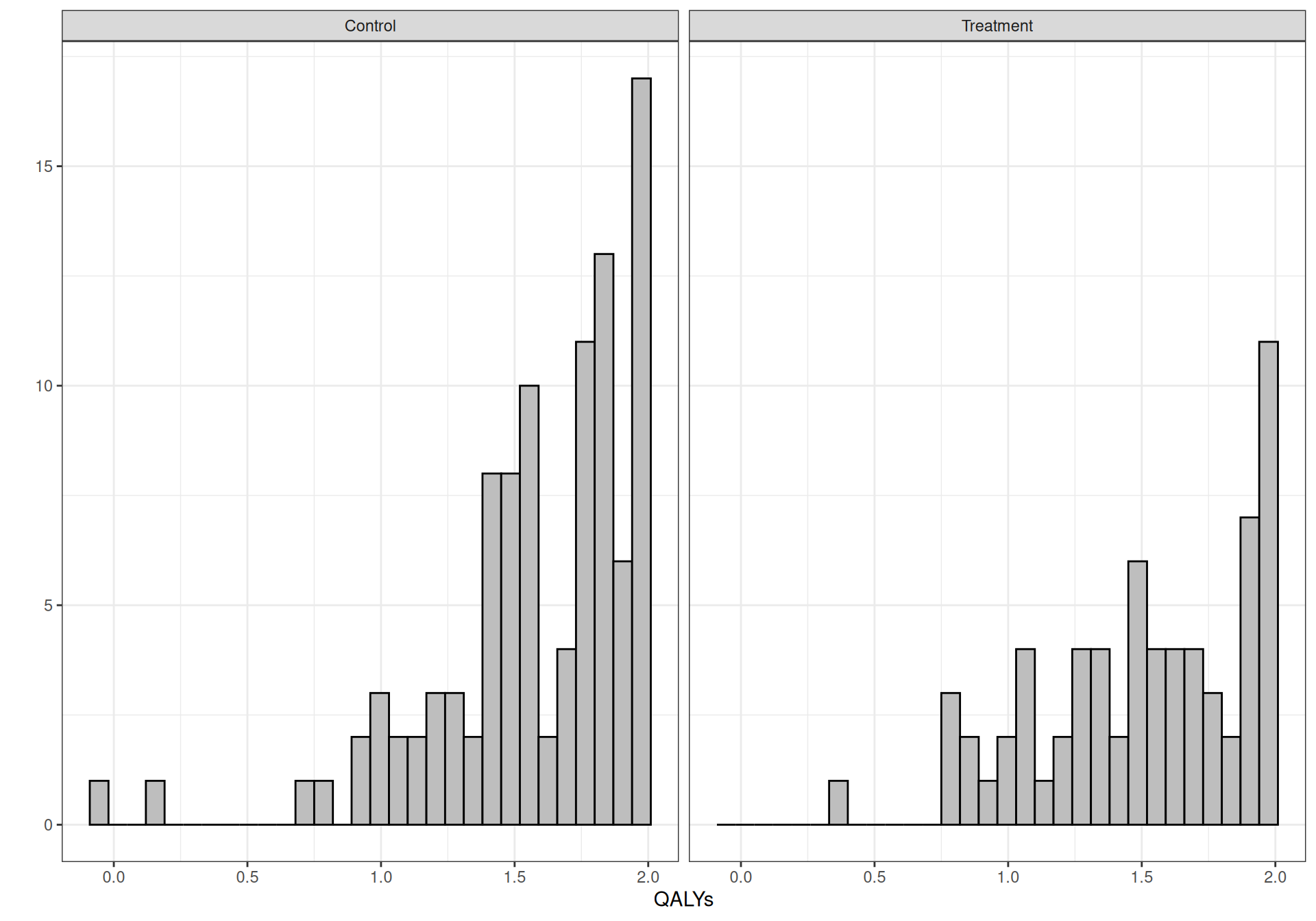
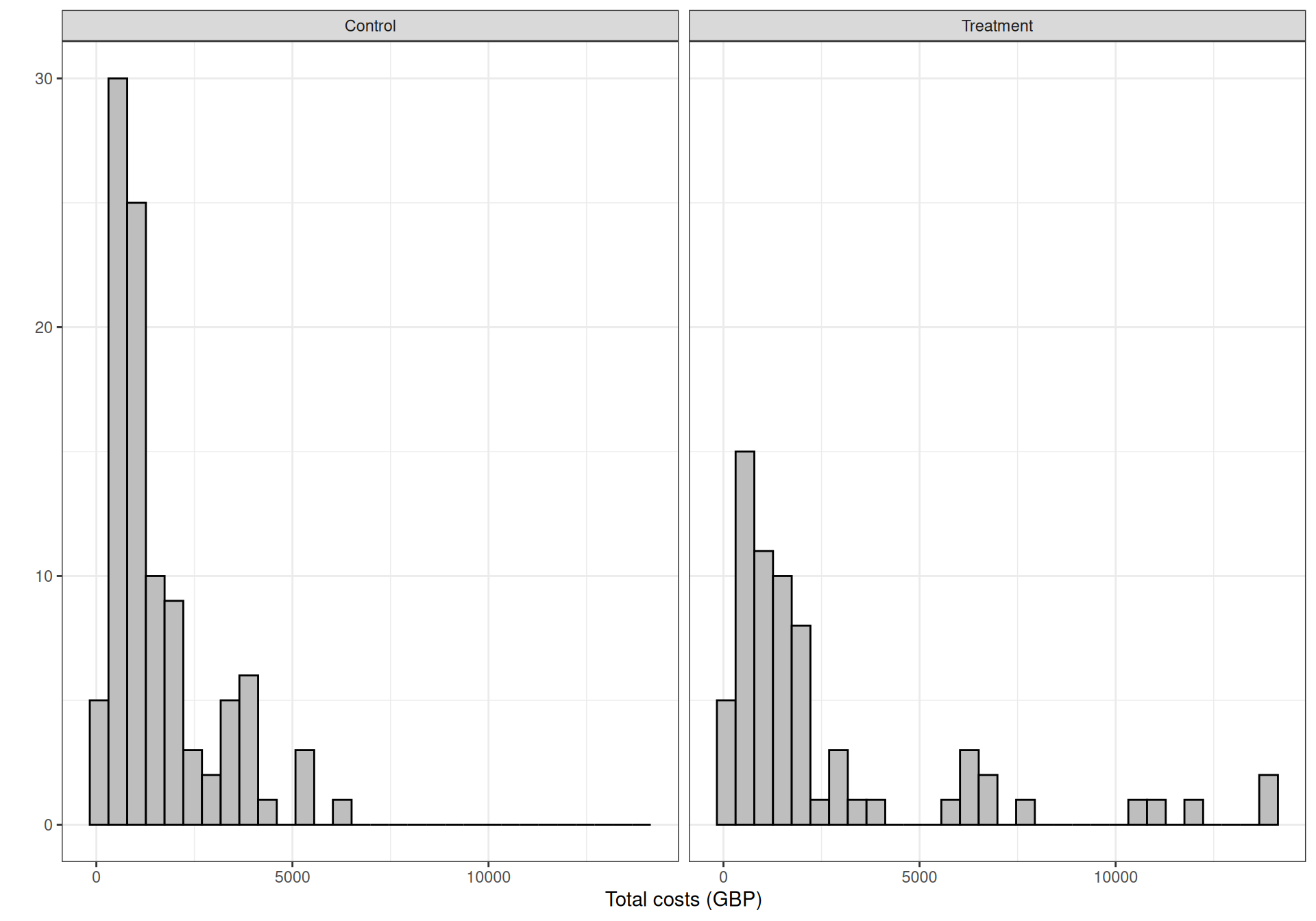
Figure 5.1 shows the histograms for the distributions of the discounted QALYs and the total costs, grouped by treatment arm. As is possible to see, the QALYs are highly skewed to the left; this is sensible, because we have a time horizon of 2 years and given the underlying disease is not life-threatening, it is reasonable to imagine that most individuals would be in a state of good health, with quite a few even in “perfect health”, resulting in very high QALYs over the two year range.

Figure 5.1: Empirical distribution for QALYs and total costs in the two treatment arms of the 10TT.

5.2 Modelling ILD in HTA

5.2.1 Normal/Normal independent model

The “standard” and most basic statistical modelling (often implicitly) assumes normality and linearity and models independently individual benefits/HRQLs and total costs by controlling for the treatment arm \(\text{Trt}_i\) and the centred baseline values, e.g. \(u_i^* = (u_i -\bar{u})\) and \(c_i^* = (c_i - \bar{c})\) \[ e_i = \alpha_{0} + \alpha_{1} \text{Trt}_i + \alpha_{2} u^*_{0i} + \varepsilon_{ei}\, [+ \ldots], \qquad \varepsilon_{ei} \sim \text{Normal}(0,\sigma_e) \tag{5.3}\] \[ c_i = \beta_{0} + \beta_{1} \text{Trt}_i + \beta_{2} c^*_{0i} + \varepsilon_{ci}\, [+ \ldots], \qquad\hspace{2pt} \varepsilon_{ci} \sim \text{Normal}(0,\sigma_c), \tag{5.4}\] where the notation \([+\ldots]\) indicates that we may want to include additional covariates in the model, for instance some demographic measurements on the individuals.

NoteStatistics vs econometrics

Equations 5.3 and 5.4 describe two linear regression models where the observable variable is expressed in terms of a “fixed” component (the linear predictor) and some random noise (the error terms \(\varepsilon_{ei}\) and \(\varepsilon_{ci}\)), in a form that is perhaps more familiar in Econometrics than it is in Statistics.

If you prefer to speak Statistics than Econometrics¹, a more common description of this model is probably to consider \[\begin{eqnarray*} e_i & \sim & \text{Normal}(\phi_{ei}, \sigma_e) \\ \phi_{ei} & = & \alpha_{0} + \alpha_{1} \text{Trt}_i + \alpha_{2} u^*_{0i} \, [+ \ldots] \end{eqnarray*}\] (of course, this extends obviously to \(c_i\)).

The two models are identical as they encode the same assumptions, in slightly different semantic ways.

Even with underlying randomised data, it is usually a good idea to control for the baseline values of utility and costs. The reason for this is that, most often, randomisation is performed with respect to the main clinical outcome \(y\), rather than to the economic ones \((e,c)\) and thus it is still possible that the baseline measurements for \((e,c)\) may be unbalanced among the different treatment or intervention arms. Using a centred version of these covariates typically simplifies the interpretation of the results (and we come back to this in Section 5.2.2).

The models in Equations 5.3 and 5.4 can produce directly an estimate of the population average effectiveness and cost differentials – under these specifications, they are directly \(\Delta_e=\alpha_{1}\) and \(\Delta_c=\beta_{1}\). In a fully frequentist/maximum likelihood analysis, we can use basic functions such as lm(), in R to obtain the estimates for the model parameters and then quantify the impact of uncertainty in model parameters on the decision making process using resampling methods, such as the bootstrap.

Example 5.2. 10TT (continued): Normal/Normal independent model. We start by modelling the 10TT data using the specification in Equations 5.3 and 5.4.

For each of the \(i=1,\ldots,N=167\) observations we model \(e_i \sim \text{Normal}(\phi_{ei},\sigma_{et})\), where \(t=1,2\) are the two intervention arm (\(t=1\) indicates the standard of care, while \(t=2\) is the active intervention – note here that we assume a treatment-specific variance). The linear predictor is defined as \[\phi_{ei} = \alpha_0 + \alpha_1 (\text{Trt}_i-1) + \alpha_2 (u_{0i}-\bar{u}_{0})\] – note that because for each individual we code in the data the treatment indicator as \(\text{Trt}_i=1,2\), we use the rescaled version \((\text{Trt}_i-1)\), so that when \(\text{Trt}_i=1\) (the control intervention), then the term disappears from the linear regression model and thus \(\alpha_1\) indicates the effect of the active intervention. In line with Equation 5.3, we control for the scaled (centred) version of the baseline HRQL, \(u^*_{0i}=(u_{0i}-\bar{u}_{0})\), whose effect is measured by the coefficient \(\alpha_2\). Consequently, we can define the population average effects as \[\mu_{et}=\alpha_0 + \alpha_1 (t-1),\] for \(t=1,2\), so that, in the control arm (\(t=1\)), the effect of the treatment disappears.

As for the costs, we model \(c_i \sim \text{Normal}(\phi_{ci},\sigma_{ct})\) and, in a similar way to what we have done for the effects, the linear predictor as \[\phi_{ci} = \beta_0 + \beta_1(\text{Trt}_i-1).\] Here, \(\beta_0\) is the value of the linear predictor \(\phi_{ci}\) when the treatment arm is \(\text{Trt}_i=1\) (i.e. the standard of care). Thus, we estimate of the population average costs as \[\mu_{ct}=\beta_0 + \beta_1(t-1),\] for \(t=1,2\). Because we only have data on the total costs over the course of the study, unlike for the effects, here we do not control for the background level.

NoteIndividual (conditional) vs population (marginal) averages

In the modelling presented above, we consider two forms of averages: the first ones are the linear predictors \(\phi_{ei}\) and \(\phi_{ci}\); because they are defined as functions of the covariates, which are measured for each individual in the sample, these represent the individual (or conditional) average benefits and costs.

Conversely, the parameters \(\mu_{et}\) and \(\mu_{ct}\), do not depend on the index \(i\), because they are constructed by averaging \(\phi_{ei}\) and \(\phi_{ci}\) over the entire range of individual profiles (i.e. combination of values for the covariates), thus identifying the population (marginal) average benefit and costs. These are the object of the economic evaluation and thus the main parameter of our analysis (we return to this point later in Section 5.2.2 and Example 5.4, as well as in Chapter 11).

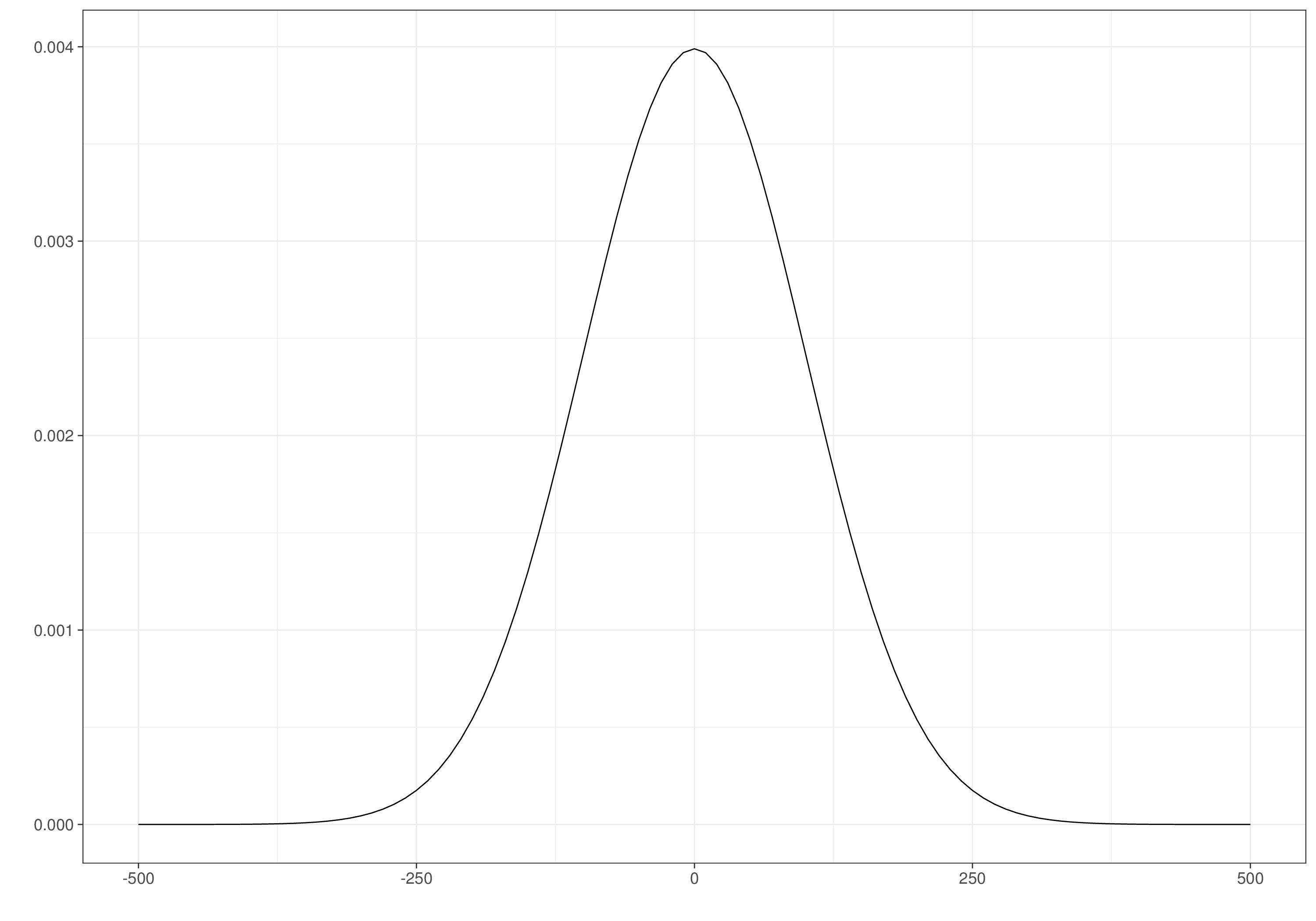
Finally, we define the prior distributions. For the regression coefficients we use minimally informative Normal priors \[\alpha_0,\alpha_1,\alpha_2,\beta_0,\beta_1 \stackrel{iid}{\sim}\text{Normal}(\text{mean}=0,\text{sd}=100)\] (this means of course a precision of \(100^{-2}=0.0001\)). Note that we could probably do much better than this – given the scale of the observed data, it is unlikely that \(\alpha_0\) and \(\alpha_1\) have such a large range. However, given we have a reasonably large sample size, this very vague prior will probably not impact on the convergence of the model (see the results below).

As for \(\beta_0\) and \(\beta_1\), in fact we need to pay a little more attention: as shown in Figure 5.1, the range of the costs is quite large: [71.34; 13 899.28], overall. For this reason, a “lazy” prior centred on 0 may fail to accommodate the full range in the data and thus place some unduly mass away from where the posterior should actually be, by effect of the observed data.

One way around this would be to use more sensible priors – after all, \(\beta_0\) indicates the average cost for the control, so we can expect it to be well away from 0 (and certainly to be positive). Alternatively and perhaps more easily, we can rescale the observed costs, e.g. by dividing them by £1000. This makes the assumption that \(\beta_0,\beta_1 \stackrel{iid}{\sim}\text{Normal}(\text{mean}=0,\text{sd}=100)\) much more sensible and allows the posterior to explore a wide enough range. Of course, when taking this approach, we need to rescale up (by a factor of £1000) the estimates for the population average costs (see also the discussion in Note 5.2, below).

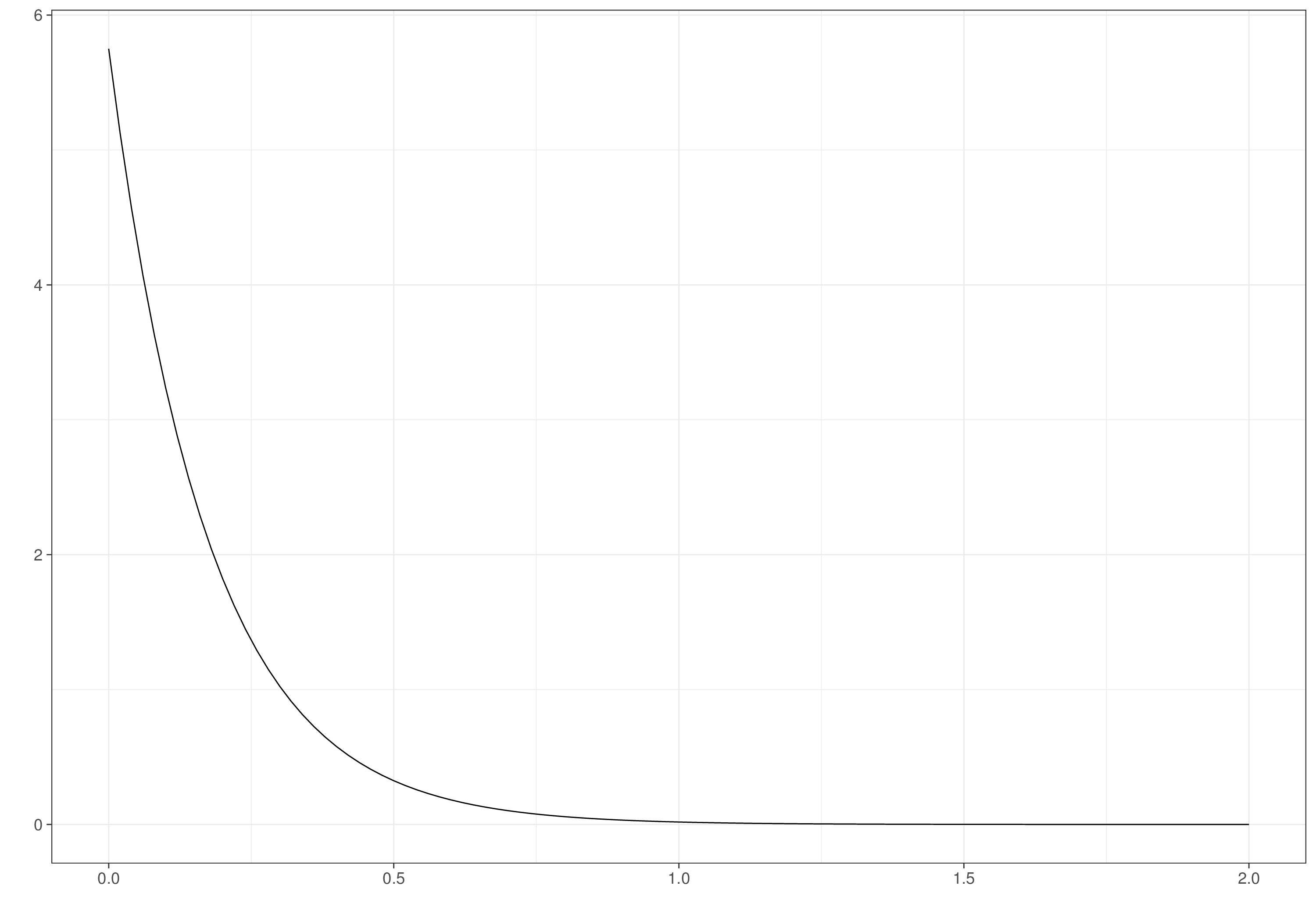
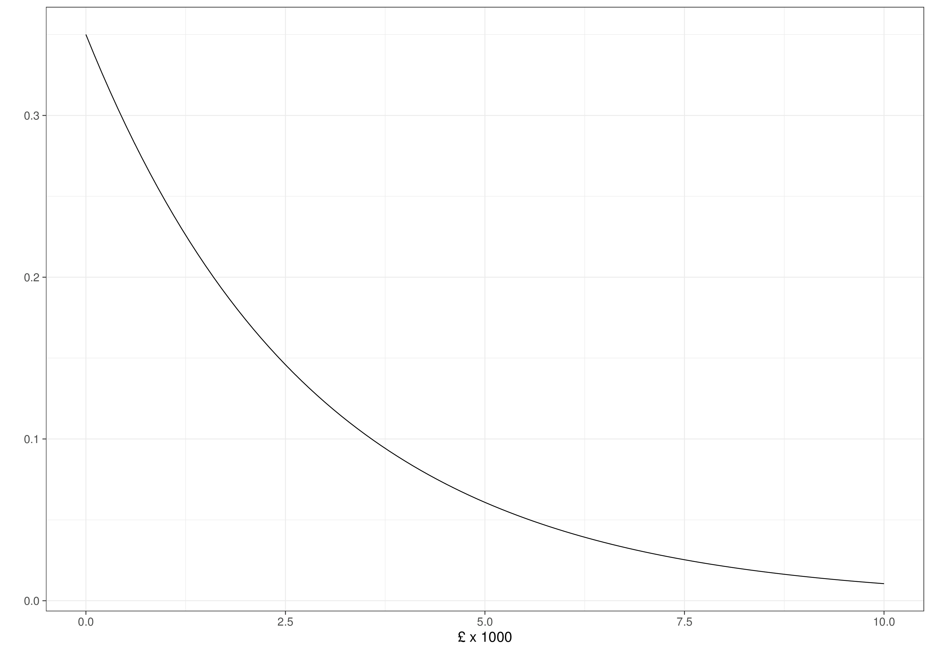
For the standard deviations for the observed costs and effects, we consider a PC prior (see Section 2.2.3 and Example 2.5 in particular). Given knowledge of the scale of the two outcomes, we assume that \(\Pr(\sigma_{et}>0.8)\approx 0.01\), leading to an Exponential distribution with rate \(-\frac{\log(0.01)}{0.8}\approx 5.75\); and, on the scale of £1000, \(\Pr(\sigma_{ct}>2)\approx 0.5\), which implies an Exponential distribution with rate \(-\frac{\log(0.5)}{2}\approx 0.35\).

Figure 5.2 shows these prior distributions. As is possible to see, the regression coefficients are widely spread and the data standard deviations have decreasingly small mass for higher values. In all cases, we do not rule out a priori the possibility that the evidence would change these distributions to different shapes.

(a) \(\alpha_0,\alpha_1,\alpha_2,\beta_0,\beta_1\).

 

(b) \(\sigma_e\).

 

(c) \(\sigma_c\).

 

Figure 5.2: The prior distributions for the parameters of the 10TT model. For \(\beta_0,\beta_1\) and \(\sigma_c\), the \(x\)–axis is scaled to £1000, given that the original data are given as \(c_i/1000\).

The full modelling assumptions under a Bayesian framework can be written into suitable JAGS code. We do so by creating an R function (as in Note 3.2 in Example 3.1).

# Normal/Normal independent model - JAGS code
nn_indep=function(){
  for (i in 1:N) {
    # Model for the effects
    e[i] ~ dnorm(phi.e[i], tau.e[Trt[i]])
    phi.e[i] <- alpha0 + alpha1*(Trt[i]-1) + alpha2*u0star[i]
    # Model for the costs
    c[i] ~ dnorm(phi.c[i], tau.c[Trt[i]])
    phi.c[i] <- beta0 + beta1*(Trt[i]-1)
  }
  # Rescales the main economic parameters 
  for (t in 1:2) {
    mu.e[t] <- alpha0 + alpha1*(t-1)
    # (NB costs need to be scaled up by 1000)
    mu.c[t] <- 1000*(beta0 + beta1*(t-1))
  }
  # Minimally informative priors on the regression coefficients
  alpha0 ~ dnorm(0,0.0001)
  alpha1 ~ dnorm(0,0.0001)
  alpha2 ~ dnorm(0,0.0001)
  beta0 ~ dnorm(0,0.0001)
  beta1 ~ dnorm(0,0.0001)
  for (t in 1:2) {
  # PC-prior on the sd with Pr(sigma_e>0.8) \approx 0.01
    sigma.e[t] ~ dexp(5.75)
    tau.e[t] <- pow(sigma.e[t],-2)
  # PC-prior on the sd with Pr(sigma_c>2) \approx 0.5
    sigma.c[t] ~ dexp(0.35)
    tau.c[t] <- pow(sigma.c[t],-2)
  }
}

Note Vectorising the linear predictor

Unlike BUGS (but similarly to other related software, such as Stan – see Section 8.3.5), JAGS allows vectorisation. This means that, instead of having to specify fully the linear predictor in a regression model, by adding all the relevant covariates, we could more economically use matrix algebra and code up the general relationship \(\mu = \boldsymbol{X}\boldsymbol\beta\), where \[ \boldsymbol{X} = \left(\begin{array}{ccccc} 1 & X_{11} & X_{12} & \cdots & X_{1C} \\ 1 & X_{21} & X_{22} & \cdots & X_{2C} \\ \vdots & \vdots & \vdots & \ddots & \vdots \\ 1 & X_{n1} & X_{n2} & \cdots & X_{nC} \end{array}\right) \] is a matrix with \(n\) rows and \(K=(C+1)\) columns (a vector of ones and then the \(C\) “active” covariates), while \(\boldsymbol\beta=(\beta_0,\beta_1,\ldots,\beta_C)\) is the vector of regression coefficients, including the intercept \(\beta_0\).

Back to the Normal/Normal independence model discussed above, we could use something like the following code to construct the covariates matrix and define the overall number of them to a variable K and then modify the JAGS code to vectorise the linear predictor.

# Pre-processing to make the matrix of covariates
X=cbind(
  rep(1,N),    # vector of 1s (intercept)
  Trt-1,       # first covariate (Treatment arm)
  u0star       # second covariate (centred baseline utility)
)
# Define number of covariates (including intercept)
K=ncol(X)

# JAGS model
nn_indep=function(){
  for (i in 1:N) {
    # Model for the effects
    e[i] ~ dnorm(phi.e[i], tau.e[Trt[i]])
    # Vectorised linear predictor using the operator %*%, which 
    # computes alpha_1*X[i,1] + alpha_2*X[i,2] + ... + alpha_K*X[i,K]
    phi.e[i] <- X[i,]%*%alpha 
    ...
  }
  # Prior on the K coefficients (including intercept)
  for (k in 1:K) {
    alpha[k] ~ dnorm(0,0.0001)
  }
  ...
}

Vectorisation means that we would not have to modify the JAGS code if we decided to include an extra covariate, or exclude an existing one – we would simply pass a different matrix X in the data list and compute a different value for K, depending on the number of its columns.

This format allows us to be more economic with setting up the priors for the regression coefficients, which we can do in a loop – and note that we do not have any restriction on assigning to each the exact same prior distribution: for example, we could index the Normal distribution for alpha[k] as a function of a specific mean mu.alpha[k] and precision tau.alpha[k], say, which would be passed on as data.

As discussed in Note 3.1 in Section 3.1.1, recall that BUGS/JAGS index the Normal distribution in terms of the precision, which we define as \(\tau_{et}=\sigma_{et}^{-2}\), to encode the assumption that each treatment arm has a specific measure of variance. Note also that we use the observed treatment indicator \(t\) to construct the index to assign to the precision. This is consistent with the prior distributions definition – the block

for (t in 1:2) {
   sigma.e[t] ~ dexp(5.75)
   tau.e[t] <- pow(sigma.e[t],-2)
   ...

specifies a separate prior for each treatment arm on the standard deviation scale and then maps it on the precision scale, which is required for BUGS/JAGS to run the model.

We now run the model using JAGS and R2jags, with the following R commands. Once the model has completed the run, we can visualise the summary statistics using the print() method for the resulting JAGS object.

# Defines the data list
data=list(e=e,c=c,Trt=Trt,u0star=u0star,N=N)

# Initialises the object 'model' as a list to store all the results
model=list()

# Runs JAGS in the background
library(R2jags)
# Stores the BUGS output as an element named 'nn_indep' in the object 'model'
model$nn_indep=jags(
  data=data,
  parameters.to.save=c(
    "mu.e","mu.c","alpha0","alpha1","alpha2","beta0","beta1","sigma.e","sigma.c"
  ),
  inits=NULL,n.chains=2,n.iter=5000,n.burnin=3000,n.thin=1,DIC=TRUE,
  # This specifies the model code as the function nn_indep()
  model.file=nn_indep
)

# Shows the summary statistics from the posterior distributions. 
print(model$nn_indep,digits=3,interval=c(0.025,0.5,0.975))

Inference for Bugs model at "/tmp/RtmpbIPSKN/modelff8ab7b9e83ba.txt", 
 2 chains, each with 5000 iterations (first 3000 discarded)
 n.sims = 4000 iterations saved. Running time = 0.541 secs
            mu.vect sd.vect     2.5%      50%    97.5%  Rhat n.eff
alpha0        1.551   0.021    1.509    1.551    1.591 1.001  4000
alpha1       -0.006   0.039   -0.082   -0.005    0.071 1.001  4000
alpha2        1.280   0.074    1.132    1.280    1.422 1.001  4000
beta0         1.561   0.134    1.299    1.560    1.824 1.001  4000
beta1         1.092   0.431    0.256    1.092    1.952 1.001  4000
mu.c[1]    1561.399 134.184 1298.523 1560.281 1823.614 1.001  4000
mu.c[2]    2653.466 414.344 1850.210 2651.108 3470.759 1.001  4000
mu.e[1]       1.551   0.021    1.509    1.551    1.591 1.001  4000
mu.e[2]       1.545   0.033    1.480    1.545    1.611 1.001  4000
sigma.c[1]    1.354   0.097    1.180    1.350    1.561 1.001  4000
sigma.c[2]    3.329   0.290    2.823    3.308    3.973 1.001  4000
sigma.e[1]    0.207   0.015    0.181    0.207    0.240 1.003   650
sigma.e[2]    0.268   0.024    0.226    0.266    0.320 1.001  2400
deviance    676.753   4.231  670.305  676.145  686.504 1.001  4000

For each parameter, n.eff is a crude measure of effective sample size,
and Rhat is the potential scale reduction factor (at convergence, Rhat=1).

DIC info (using the rule: pV = var(deviance)/2)
pV = 9.0 and DIC = 685.7
DIC is an estimate of expected predictive error (lower deviance is better).

The weird path for the model file (in this case /tmp/RtmpbIPSKN/modelff8ab7b9e83ba.txt) depends on the fact that we are coding up the model as a function. JAGS will write data and model files onto a temporary folder (/tmp/RtmpbIPSKN, in this case).

As is possible to see from the summary statistics, convergence seems to be reached for all the model parameters and, according to the ESS (see Section 2.3.2.2) is reasonably large for almost all the parameters, indicating that there are no crucial issues with autocorrelation. We can use bmhe and other packages to produce other diagnostics visualisations and summaries, as in Section 2.3.2.

The intervention seems to produce slightly lower QALYs than the standard of care (on average, 1.545 against 1.551). These differences do not seem substantial, though, with much of the underlying distributions crossing each other. The difference in population average costs seem to be more marked, with average values of £\(2653.47\) against £\(1561.4\). As mentioned above, these relative differences are equivalent to the observed posterior values for the regression parameters \(\alpha_1\) and \(\beta_1\).

The posterior summaries for the parameters \(\sigma_{et}\) and \(\sigma_{ct}\) indicate that the evidence from the data perhaps is stronger than implied in the prior, with the former shrunk towards smaller values and the latter pushed to higher ones. Then again, the PC priors are able to not force too much information and can be modified if a strong signal is observed in the data.

The first important issue with the basic structure described above is that it fails to account for the potential correlation between costs and clinical benefits. In general, this may materialise as a positive correlation, since effective treatments are innovative and result from intensive and lengthy research and are thus associated with higher unit costs. However, it may also arise as negative correlation, because more effective treatments may end up reducing total care pathway costs e.g. by reducing hospitalisations, side effects, etc.

Either way, modelling costs and benefits separately and (more or less implicitly) assuming independent error terms in the regression models in Equations 5.3 and 5.4 simply fails to allow for the possibility of correlation, potentially leading to biased estimates.

In a frequentist/maximum likelihood setting, one possible way around this limitation is to use so-called “seemingly unrelated regression” (SUR) models, originally proposed by Zellner (1962). SUR models essentially imply a correlation structure between the error terms \((\varepsilon_{ei},\varepsilon_{ci})\) – this is effectively the same model as in Equations 5.3 and 5.4, but with the added assumption that \[\left( \begin{array}{c} \varepsilon_{ei} \\ \varepsilon_{ci}\end{array} \right) \sim \text{Normal}\left( \left(\begin{array}{c} 0 \\ 0\end{array}\right), \left(\begin{array}{cc} \sigma^2_e & \rho\sigma_e\sigma_c \\ & \sigma^2_c \end{array}\right) \right).\] Earlier advice on statistical modelling for HTA did consider this – see for instance Willan and Briggs (2006).

A second potential issue is that joint or marginal normality is generally not a realistic assumption. This is because costs are usually skewed and certainly bounded in \([0; \infty)\), while benefits may be bounded in an interval \([a; b]\), for some problem-specific constants, e.g. when representing QALYs – see Figure 5.1.

One obvious solution to this would be to use suitable transformations, for instance to model \(\log c_i\) to make the Normal sampling distribution more plausible; while this is reasonably easy to do, care is needed when back transforming to the natural scale – see also Section 5.2.3 and recall that the objectives of the economic evaluation are the population average (mean) cost and benefits, because it is them we need to feed to the decision analysis (see Chapter 4). We return to this problem in Example 5.4 and in Section 5.2.3.

5.2.2 Marginal/conditional factorisation model

To overcome the issues highlighted above, we can take a set of countermeasures, which allow us to build models capable of producing estimates of the population average cost and benefit accounting for potential correlation as well as for the underlying nature of the observed data. This is of course an important objective – but it does mean using a much more structured modelling framework, as we explain below.

The main objective is to consider as target for our inference the joint probability distribution \(p(e,c\mid\boldsymbol\theta)\), for some vector of model parameters \(\boldsymbol\theta\). A useful strategy that allows us to move away from the normality assumption without too many complications makes use of the fundamental properties of probability, under which we can always factorise a joint distribution into the product of a (univariate) marginal and a (univariate) conditional: \[p(e,c)=p(e)p(c\mid e) = p(c)p(e\mid c) \tag{5.5}\] – note that we temporarily drop the dependence to the model parameters, for simplicity. We label this modelling strategy as “marginal/conditional factorisation” (MCF) model.

From a purely probabilistic point of view, the two different factorisations are equivalent and represent fully the target joint distribution. Pragmatically, we may have some underlying causal construct, whereby, for instance, it is more appropriate to think of a DGP in which the effects have an impact on the costs (and thus we may favour the first factorisation in Equation 5.5).

Figure 5.3 shows a graphical representation of this structured modelling framework – indeed, we assume that the joint is factorised as \(p(e,c\mid\boldsymbol\theta)=p(e\mid\boldsymbol\theta_e)p(c\mid e,\boldsymbol\theta_c)\), for some specific subset of parameters \(\boldsymbol\theta=(\boldsymbol\theta_e,\boldsymbol\theta_c)\). The dashed box indicates the marginal model for the benefits \(e_i \sim p(e \mid \phi_{ei},\boldsymbol\xi_e)\). Here, \(\boldsymbol\theta_e=(\phi_{ei},\boldsymbol\xi_e)\); \(\phi_{ei}\) is a location parameter indicating a measure of central tendency for the underlying distribution, while \(\boldsymbol\xi_e\) is a set of ancillary parameters, which may indicate a measure of shape, or variance – these may or may not be present, depending on the form of the distribution \(p(\cdot)\) that we choose. We can model the location parameter using some generalised linear regression \[g_e(\phi_{ei}) = \alpha_0 + \alpha_1 \text{Trt}_i \, [+\ldots]. \tag{5.6}\]

Figure 5.3: A DAG representation of the marginal/conditional factorisation model for effects and costs (aligned with the formulation in Equations 5.6 and 5.7).

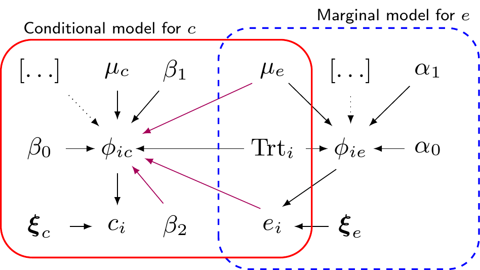
The solid box in Figure 5.3 shows the conditional model for the cost, given the effects. We describe \(c_i\sim p_c(c \mid e,\phi_{ci},\boldsymbol\xi_c)\), where, again, \(\phi_{ci}\) is a location and \(\boldsymbol\xi_c\) is a vector of ancillary parameters. We include the dependence between costs and effects through the location parameter, which is again modelled using a generalised linear regression \[g_c(\phi_{ci})=\beta_0 + \beta_1\text{Trt}_i + \beta_2 \left(e_i - \mu_e\right)\, [+\ldots], \tag{5.7}\] where this time we definitely have one (centred) covariate, i.e. the observed individual benefits, scaled by the estimated population average (which we get from the previous module).

In Equation 5.7, the coefficient \(\beta_2\) quantifies the level of correlation between \(e\) and \(c\) – in the simplest case of a Normal/Normal model (which we describe in more details in Example 5.3), we can prove analytically the relationship \[\beta_2 = \rho \frac{\sigma_c}{\sigma_e} \qquad\Rightarrow\qquad \rho = \beta_2\frac{\sigma_e}{\sigma_c}, \tag{5.8}\] where \(\rho\in(-1,1)\) is the linear correlation coefficient between costs and benefits (see Example 5.3).

It is very much possible that the evidence in the data suggests that, in fact, there is no substantial correlation among the two outcomes and thus the estimate for its value would be close to 0 – in a frequentist setup, this would be “non-significantly different from 0”. On the other hand, the model does allow for the possibility that the two outcomes are indeed correlated and if the evidence supported this assumption, then \(\beta_2\) would be estimated with a value away from 0.

In addition, the modelling structure encoded in Figure 5.3 do make the simplifying assumption that the correlation between costs and benefits only happens through the location parameter. However, this is by no means a requirement and it would be possible to add even further structure and build another generalised linear regression component in which \(\boldsymbol\xi_c\) does depend probabilistically on \(e_i\). We make a similar remark in the context of survival modelling, in Section 8.3.3.

If no further covariates are included in the two generalised linear regressions of Equations 5.6 and 5.7, we compute \(\mu_{et}=g_e^{-1}\left(\alpha_0 + \alpha_1 (t-1)\right)\) and \(\mu_{ct}=g_c^{-1}\left(\beta_0 + \beta_1 (t-1) \right)\) – i.e. setting \(\left(e_i - \mu_e\right)=0\) to obtain the average cost in correspondence of the average benefits profile.

If we do consider additional covariates in Equations 5.6 and/or 5.7, we can still use the rescaled intercepts to estimate the population average benefits and costs. However, in this case, the two models target directly two conditional estimates, given the “profile” of covariates and so a little care is needed.

For example, consider the case \[g_e(\phi_{ei}) = \alpha_0+\alpha_1 \text{Trt}_i + \alpha_2 (u_{0i}-\bar{u}_0) + \alpha_3 \text{Sex}_i,\] where \((u_{0i}-\bar{u}_0)\) is the centred baseline HRQL continuous measurement and \(\text{Sex}_i\) is a discrete variable taking values \((0,1)\) for males and females, respectively. Under this specification, \(g_e^{-1}\left(\alpha_0 + \alpha_1 (t-1)\right)=\) population average benefits for a male with average baseline HRQL measurement, while \(g_e^{-1}\left(\alpha_0+\alpha_1(t-1) + \alpha_3\right)=\) population average benefits for a female with average baseline HRQL measurement. We can approximate the marginal population average benefit as \[ \mu_{et}\approx p_M g_e^{-1}\left(\alpha_0+\alpha_1 (t-1)\right) + p_F g_e^{-1}\left(\alpha_0+\alpha_1(t-1) +\alpha_3\right), \tag{5.9}\] where \(p_M\) and \(p_F\) are the frequencies with which males and females are observed in the population of interest. Note that marginalisation of continuous covariates is automatic with centring (because it makes sense to determine the “average” profile, with respect to these covariates). Conversely, for discrete covariates we need to effectively compute a weighted average over their levels – we return to the distinction between marginal and conditional estimates in Example 11.2 in Section 11.3.1.

NoteTo be or not to be… (Bayesian)?

While there is nothing inherently Bayesian about the modelling framework described in Figure 5.3, there are several advantages to using a Bayesian approach.

1. As the model becomes more and more realistic and its structure more and more complex, to account for skeweness and correlation, the computational advantages of using maximum likelihood estimations become increasingly smaller. This is because writing and optimising the likelihood function becomes more complex analytically and even numerically and might require the use of simulation althorithms. A Bayesian approach, conversely, can scale up with minimal changes – whether we consider the simple Normal-Normal model or more convoluted distributional assumptions, MCMC methods effectively require almost no modification. The computation may be more expensive, but the marginal computational cost is in fact diminishing.
2. As mentioned above, it is very possible that realistic models be based on highly non-linear transformations; from a Bayesian perspective, this does not pose a substantial problem, because once we obtain simulations from the posterior distribution for \(\alpha_0\) and \(\beta_0\), it is possible to simply rescale them to obtain samples from the posterior distribution of \(\mu_e\) and \(\mu_c\). This in turn allows us to fully characterise and propagate the uncertainty in the fundamental economic parameters to the rest of the decision analysis with essentially no extra computational cost. A frequentist/maximum likelihood approach would resort to resampling methods, such as the bootstrap to effectively produce an approximation to the joint posterior distribution for all the model parameters \(\boldsymbol\theta\) and any function thereof.
3. Prior information can help stabilise inference (especially with sparse data, as shown in Example 1.2). Most often, we do have contextual information to mitigate limited evidence from the data and stabilise the evidence – for instance, we may be confident in thinking that odds ratio for drug-related treatment effects are rarely very large (say, larger than 1.5 or 2 — see Note 6.2 in Example 6.3); similarly, when looking at time-to-event data, we know for instance that cancer patients are unlikely to outlive the general population and thus we may “anchor” estimates for sick individuals using population life tables. Using a Bayesian approach allows us to use this contextual information in a principled way.

Example 5.3. 10TT (continued): Normal/Normal MCF model. The simplest version of the modelling framework of Figure 5.3, which is equivalent to a standard implementation of the SUR model, is: \[\begin{align*} e_i \sim \text{Normal}(\phi_{ei},\tau_{et}) && \phi_{ei} &= \alpha_0 +\alpha_1(\text{Trt}_i-1) + \alpha_2 u^*_{0i} && \mu_{et} = \alpha_0 + \alpha_1(t-1) \\ c_i\mid e_i \sim \text{Normal}(\phi_{ci},\tau_{ct}) && \phi_{ci} &= \beta_0 + \beta_1(\text{Trt}_i-1) + \beta_2(e_i -\mu_e) && \mu_{ct} = \beta_0 + \beta_1(t-1), \end{align*}\] where \(\phi_{ei}\) and \(\tau_e\) are the benefits marginal mean and precision, respectively, while \(\phi_{ci}\) and \(\tau_c\) are the costs conditional mean and precision, respectively. In this model, the ancillary parameters are \(\xi_e=\tau_e\) and \(\xi_c=\tau_c\) and both \(g_e(\cdot)\) and \(g_c(\cdot)\) are the identity function and so the two intercepts represent directly the population average parameters.

Note that, in this particular case, because we are using rescaled data on \(c_i\), the population average cost also needs to be rescaled up by £1000 and thus \(\mu_{ct} = 1000\left(\beta_0 + \beta_1(t-1)\right)\).

This formulation is indeed fairly similar to that of Equations 5.3 and 5.4, with the notable improvement that we no longer assume independence across the outcomes, because of the inclusion of the term \(\beta_1(\text{Trt}_i-1)\) in the linear predictor for the location parameter of the conditional cost distribution.

While perhaps less intuitive, at face value, than a bivariate distribution, the modelling framework of Figure 5.3 has the advantage that the two components in which we factorise the joint distribution have lower dimension – we do not need to model a bivariate distribution, but two univariate ones.

NoteWhat’s so special about the Normal distribution?…

One of the nice features of the Normal distribution is that, given a joint, multivariate Normal for a \(K\)-dimensional vector \(\boldsymbol{y}=(y_1,\ldots,y_K) \sim \text{Normal}_K(\boldsymbol\mu,\boldsymbol\Sigma)\), then we can prove that all the resulting marginal and conditional distributions remain Normal.

Specifically, in the bivariate case of interest in HTA \[\left(\begin{array}{c} e \\ c \end{array}\right) \sim \text{Normal}_2\left(\left(\begin{array}{c} \mu_e \\ \mu_c\end{array} \right), \left(\begin{array}{cc} \sigma^2_e & \rho\sigma_e\sigma_c \\ & \sigma^2_c \end{array} \right) \right)\] we can prove that \[e \sim \text{Normal}(\mu_e,\sigma_e) \quad \mbox{and} \quad c\mid e \sim \text{Normal}\left(\eta_c,\lambda_c \right),\] where \[\eta_c=\mu_c+\rho\frac{\sigma_c}{\sigma_e}(e-\mu_e)\] is the conditional mean and \[\lambda_c = \sqrt{(1-\rho^2)\sigma^2_c}, \tag{5.10}\] is the conditional standard deviation for the costs, both defined as functions of the marginal means \(\mu_e,\mu_c\), the marginal standard deviations \(\sigma_e,\sigma_c\) and the correlation coefficient \(\rho\). Of course we can derive the other factorisation with a marginal for \(c\) and a conditional \(e\mid c\), accordingly.

This property, specific to the Normal distribution, implies that the Normal/Normal MCF model is indeed equivalent to the SUR model.

The modelling assumptions detailed above can be encoded in the JAGS code below.

# Normal/Normal MCF - JAGS code
nn_mcf=function(){
  for (i in 1:N) {
    # Marginal model for the effects
    e[i] ~ dnorm(phi.e[i], tau.e[Trt[i]])
    phi.e[i] <- alpha0 + alpha1*(Trt[i]-1) + alpha2*u0star[i]
    # *Conditional* model for the costs
    c[i] ~ dnorm(phi.c[i], tau.c[Trt[i]])
    phi.c[i] <- beta0 + beta1*(Trt[i]-1) + beta2*(e[i]-mu.e[Trt[i]]) 
  }
  # Rescales the main economic parameters
  for (t in 1:2) {
    mu.e[t] <- alpha0 + alpha1*(t-1)
    # (NB costs need to be scaled up by 1000)
    mu.c[t] <- 1000*(beta0 + beta1*(t-1))
  }
  # Minimally informative priors on the regression coefficients
  alpha0 ~ dnorm(0,0.0001)
  alpha1 ~ dnorm(0,0.0001)
  alpha2 ~ dnorm(0,0.0001)
  beta0 ~ dnorm(0,0.0001)
  beta1 ~ dnorm(0,0.0001)
  beta2 ~ dnorm(0,0.0001)
  for (t in 1:2) {
  # PC-prior on the *marginal* sd with Pr(sigma_e>0.8) \approx 0.01
    sigma.e[t] ~ dexp(5.75)
    tau.e[t] <- pow(sigma.e[t],-2)
  # PC-prior on the *conditional* sd with Pr(lambda_c>2) \approx 0.5
    lambda.c[t] ~ dexp(0.35)
    tau.c[t] <- pow(lambda.c[t],-2)
  # Retrieves the correlation coefficients
    rho[t] <- beta2*sigma.e[t]/sigma.c[t]
  # And the *marginal* standard deviation for the cost
    sigma.c[t] <- sqrt(pow(lambda.c[t],2) + pow(sigma.e[t],2)*pow(beta2,2))
  }
}

Because of the underlying assumption of joint Normality, we can write down analytically and monitor the posterior distributions for the correlation coefficient rho[t] and the marginal cost standard deviation sigma.c[t], obtained using Equation 5.8 and combining it with Equation 5.10.

In reality, defining and monitoring rho[t] and sigma.c[t] is not essential – we can do it analytically in the bivariate Normal case and thus we show how to handle this in the code above. But, realistically, for the purposes of the HTA analysis, we do not care massively about them and could dispense with this extra computation.

The model is run using the following code.

# Runs JAGS in the background and stores the output in the element 'nn_mcf' 
model$nn_mcf=jags(
  data=data,
  parameters.to.save=c(
    "mu.e","mu.c","alpha0","alpha1","alpha2","beta0","beta1","beta2",
    "sigma.e","sigma.c","lambda.c","rho"
  ),
  inits=NULL,n.chains=2,n.iter=5000,n.burnin=3000,n.thin=1,DIC=TRUE,
  # This specifies the model code as the function nn_mcf()
  model.file=nn_mcf
)

# Shows the summary statistics from the posterior distributions. 
print(model$nn_mcf,digits=3,interval=c(0.025,0.5,0.975))

Inference for Bugs model at "/tmp/RtmpbIPSKN/modelff8ab4fc37ba1.txt", 
 2 chains, each with 5000 iterations (first 3000 discarded)
 n.sims = 4000 iterations saved. Running time = 0.775 secs
             mu.vect sd.vect     2.5%      50%    97.5%  Rhat n.eff
alpha0         1.551   0.021    1.510    1.551    1.592 1.001  4000
alpha1        -0.005   0.040   -0.083   -0.005    0.071 1.001  4000
alpha2         1.280   0.073    1.139    1.280    1.425 1.002  1700
beta0          1.592   0.134    1.337    1.587    1.863 1.001  4000
beta1          1.003   0.421    0.188    0.992    1.840 1.002  1500
beta2         -1.189   0.322   -1.833   -1.187   -0.574 1.001  4000
lambda.c[1]    1.303   0.094    1.132    1.297    1.503 1.001  2000
lambda.c[2]    3.223   0.286    2.722    3.201    3.848 1.002  1200
mu.c[1]     1592.250 133.591 1337.432 1587.482 1863.447 1.001  4000
mu.c[2]     2594.857 392.871 1820.050 2590.416 3376.337 1.002  1300
mu.e[1]        1.551   0.021    1.510    1.551    1.592 1.001  4000
mu.e[2]        1.545   0.033    1.480    1.545    1.612 1.001  4000
rho[1]        -0.186   0.051   -0.288   -0.185   -0.088 1.001  4000
rho[2]        -0.099   0.030   -0.162   -0.097   -0.046 1.001  4000
sigma.c[1]     1.327   0.094    1.157    1.322    1.527 1.001  2300
sigma.c[2]     3.240   0.284    2.744    3.219    3.863 1.002  1100
sigma.e[1]     0.207   0.015    0.180    0.206    0.239 1.001  3800
sigma.e[2]     0.267   0.023    0.226    0.265    0.319 1.002  1900
deviance     664.258   4.435  657.357  663.652  674.319 1.002  1600

For each parameter, n.eff is a crude measure of effective sample size,
and Rhat is the potential scale reduction factor (at convergence, Rhat=1).

DIC info (using the rule: pV = var(deviance)/2)
pV = 9.8 and DIC = 674.1
DIC is an estimate of expected predictive error (lower deviance is better).

Looking at the summary table produced by JAGS, we can see that convergence and autocorrelation are not a problem. All \(\hat{R}\) statistics are well below the rule-of-thumb threshold of 1.1 (see Section 2.3.2.1) and the effective sample size (Section 2.3.2.2) is generally close to the nominal one, for almost all the monitored nodes.

Note (Non-essential) Computed parameters in BUGS/JAGS

In fact, we do not even need to include the definition for the nodes rho[t] and sigma.c[t] in the JAGS model, because these are simply deterministic functions of other model parameters (beta2, sigma.e[t], and lambda.c[t]). Thus, if we run the model by monitoring these key nodes, we can actually construct rho[t] and sigma.c[t] in R using simple algebra.

Note that BUGS/JAGS effectively adds a dimension to each node. So the node beta2 is defined in the model code as a scalar, but because when processed by BUGS/JAGS we record n.sims simulations, then the resulting object turns into a vector with n.sims rows. Similarly, in the model code lambda.c is a vector with two elements (one for each treatment arm) and therefore when processed by BUGS/JAGS the element model$nn_mcf$sims.list$sigma.e is in fact a matrix with n.sims rows and 2 columns.

For this reason, when defining in R the new nodes sigma.c and rho we need to set them to matrices – and for convenience we can use the same dimension as lambda.c, as shown in the code below.

# Extracts the simulations from the BUGS object into R variables
lambda.c=model$nn_mcf$BUGSoutput$sims.list$lambda.c 
sigma.e=model$nn_mcf$BUGSoutput$sims.list$sigma.e
beta1=model$nn_mcf$BUGSoutput$sims.list$beta1

# Defines the new variables -- note the dimensions!
sigma.c=rho=matrix(NA,nrow=nrow(lambda.c),ncol=ncol(lambda.c))

# Uses the simulated values to compute rho[t] and sigma.c[t]
for (t in 1:2) {
  sigma.c[,t]=sqrt(lambda.c[,t]^2 + (sigma.e[,t]^2*beta1^2))
  rho[,t]=beta1*sigma.e[,t]/sigma.c[,t]
}

# Summarises the results
colnames(sigma.c)=c("sigma.c[1]","sigma.c[2]")
colnames(rho)=c("rho[1]","rho[2]")
cbind(sigma.c,rho) |> bmhe::stats() |> round(digits=3)

            mean    sd  2.5% median 97.5%
sigma.c[1] 1.322 0.093 1.151  1.319 1.521
sigma.c[2] 3.236 0.285 2.739  3.216 3.858
rho[1]     0.157 0.066 0.029  0.156 0.290
rho[2]     0.083 0.036 0.015  0.082 0.156

As is possible to see in the summary table produced by R, the results are (of course!) identical with the ones reported directly by JAGS.

Most of the times, it does not really matter which way around we decide to make the algebraic calculation, However, it is perhaps good practice to leave all the non-essential non-MCMC computation to R, because BUGS/JAGS models scale up in computational complexity with the number of nodes defined. If the model is fairly quick to run, as in the present case, there really is not much difference; but for more structured models, it may be much more efficient to leave some of the computation back to R.

The correlation coefficients are estimated to be very small and with rather large variance. However, in frequentist parlance, they would be deemed to be “significant”, because their posterior distribution has most of the mass below the threshold value of 0. This is consistent with the slight differences in the estimates for the conditional and the marginal standard deviations for the costs (lambda.c and sigma.c). These translate into slight differences in the estimates for the overall population average costs, although, on this occasion, these are fairly minor.

This is a reassuring feature of the MCF model – if there is no evidence of correlation in the data, we do not lose anything in comparison to the independence model of Example 5.2, because the resulting correlation is effectively set to 0, meaning that the two modules in Figure 5.3 become detached. If however, there is correlation in the data but we do not allow our model to pick it up we may end inducing important bias in our estimates.

Figure 5.4 shows a comparison of the Normal/Normal independent and the Normal/Normal MCF models. As is possible to see, the estimates for the model parameters are effectively identical – this is consistent with the discussion above, because with limited correlation, the two models more or less coincide.

(a)

(b)

Figure 5.4: Graphical summaries of the posterior distributions for the model parameters. The two panels collect parameters according to the range of their distributions, for better visualisation. The dots indicate the posterior means, while the lines expands to cover the 95% posterior intervals. Darker dots and lines indicate the Normal/Normal independence model, while lighter dots and lines indicate the Normal/Normal MCF model. 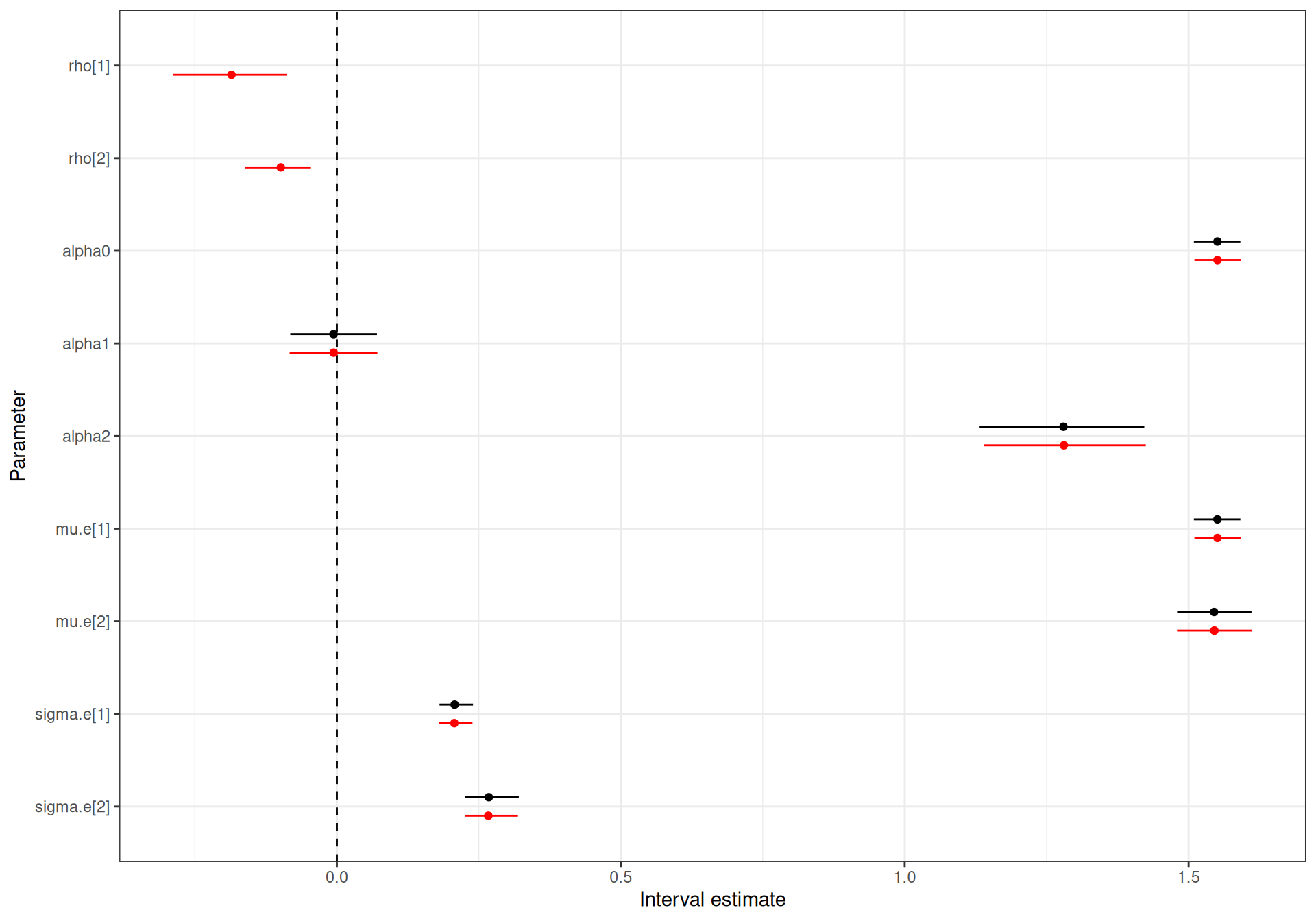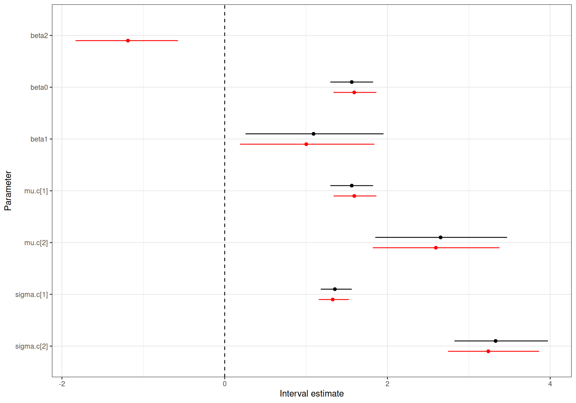For consistency in the visualisation, the parameters mu.c[1] and mu.c[2] are scaled down by a factor of 1000.

Using the structure described in Figure 5.3 it is possible to easily extend the Normal/Normal MCF model to virtually consider any combination of distributional assumptions for the costs and benefits. For example, we can assume a Gamma distribution to model skewed, positive costs, conditionally on a suitable measure of benefits; or a Beta distribution to model marginal benefits defined in terms of QALYs for a study where the time horizon is below 1 year – assuming there are no individuals with negative QALYs, implies that the range for the variable \(e\) would be between \((0,1)\).

Example 5.4. 10TT (continued): Gamma/Gamma MCF model. Figure 5.1 clearly shows that the empirical distributions for both costs and benefits are highly skewed. In addition, because the time horizon for the study is 24 months, the QALYs are naturally constrained to be below 2. For these reasons, it is a good idea to try and use non-Normal models.

One slight complication is that the QALYs show a rather large left skewness; in addition, a small number of individuals are associated with negative QALYs, indicating a very poor health state (“worse than death”). For these reasons, it is helpful to transform the original data, so that we can apply a simpler model. Following Gabrio et al. (2025), we define the transformation \(e^*_i = (3 -e_i)\). This rescales the observed QALYs and turns the distribution into a right skewed one, which means we can appropriately use a Gamma distribution to model the sampling variability. We return to this point in Note 5.2 in Section 5.3.1.

With this, we can model: \[\begin{align*} e^*_{i} \sim \text{Gamma}(\nu_e,\gamma_{ei}) && & \log(\phi_{ei}) = \alpha_0 + \alpha_1(\text{Trt}_i-1) + \alpha_2 u^*_{0i}\\ c_i\mid e^*_i \sim \text{Gamma}(\nu_c,\gamma_{ci}) && & \log(\phi_{ci}) = \beta_0 + \beta_1(\text{Trt}_i-1) + \beta_2(e^*_i -\mu^*_e), \end{align*}\] where, because of the properties of the Gamma distribution, \(\phi_{ei}\) indicates the marginal mean for the QALYs, while \(\nu_e\) is the shape and \(\gamma_{ei}=\nu_c/\phi_{ei}\) is the rate (see Section 1.2.3 and Equation 1.8, in particular). Similarly, \(\nu_c\) is the shape and \(\gamma_{ci}=\nu_c/\phi_{ci}\) is the rate of the conditional distribution for the costs given the benefits, with \(\phi_{ci}\) representing the conditional mean.

The population average benefits and costs can be retrieved by back-transforming the linear predictors (using the exponential function) \[\mu^*_e = \exp\left(\alpha_0 + \alpha_1(t-1)\right) \quad \mbox{and}\quad \mu_ c = \exp\left(\beta_0 + \beta_1(t-1)\right),\] though, of course, as we are still using rescaled data, in this instance the population average costs are computed as \(\mu_ c = \text{\pounds} 1000 \exp\left(\beta_0 + \beta_1(t-1)\right)\) – see again Note 5.2 in Section 5.3.1.

In terms of prior distributions, we keep the very vague, minimally informative priors for the regression coefficients – again, we could probably do better here, considering that both \(\phi_{ei}\) and \(\phi_{ci}\) are defined on a log scale and thus we are implying a very large range in the priors. Sensitivity analysis may be very important to this aspect.

As for the shape parameters \(\nu_{et}\) and \(\nu_{ct}\), we specify again a PC prior. Generally speaking, it is more difficult to encode genuine prior knowledge on this scale (see the discussion in Section 1.2.3) and thus we start by including a fairly vague specification, where we assume that \(\Pr(\nu_{et}>30)=\Pr(\nu_{ct}>30)\approx 0.01\), which implies an Exponential with rate \(-\frac{\log(0.01)}{30}\approx 0.15\).

The modelling assumptions are mapped onto the JAGS code below.

# Gamma/Gamma MCF - JAGS code
gg_mcf=function(){
  for (i in 1:N) {
   # Marginal model for the *rescaled* effects
   estar[i] ~ dgamma(nu.e[Trt[i]], gamma.e[Trt[i],i])
   gamma.e[Trt[i],i] <- nu.e[Trt[i]]/phi.e[i]
   log(phi.e[i]) <- alpha0 + alpha1*(Trt[i]-1) + alpha2*u0star[i]
   # Conditional model for the costs
   c[i] ~ dgamma(nu.c[Trt[i]], gamma.c[Trt[i],i])
   gamma.c[Trt[i],i] <- nu.c[Trt[i]]/phi.c[i]
   log(phi.c[i]) <- beta0 + beta1*(Trt[i]-1) + beta2*(estar[i]-mustar.e[Trt[i]]) 
  }
  # Rescales the main economic parameters
  for (t in 1:2) {
   mustar.e[t] <- exp(alpha0 + alpha1*(t-1))
   mu.e[t] <- 3 - mustar.e[t]
   # (NB costs need to be scaled up by 1000)
   mu.c[t] <- 1000*exp(beta0 + beta1*(t-1))
  }
  # Minimally informative priors on the regression coefficients
  alpha0 ~ dnorm(0,0.0001)
  alpha1 ~ dnorm(0,0.0001)
  alpha2 ~ dnorm(0,0.0001)
  beta0 ~ dnorm(0,0.0001)
  beta1 ~ dnorm(0,0.0001)
  beta2 ~ dnorm(0,0.0001)
  # PC prior on the shape parameters 
  # assume that Pr(nu.e>30) = Pr(nu.c>30) \approx 0.01
  for (t in 1:2) {
    nu.e[t] ~ dexp(0.15)
    nu.c[t] ~ dexp(0.15)
  }
}

Notice that in the code above we first define the variable mustar.e to indicate the population average QALYs on the rescaled version and then back-transform to the original scale by simply using the command mu.e[t] <- 3 - mustar.e[t]. This is possible because the transformation applied to the original data is linear and thus it holds for the expectations \[e^* = 3-e \quad \Rightarrow \quad \text{E}[e^*] = \text{E}[3-e] = 3 - \text{E}[e] \quad \Rightarrow \quad \text{E}[e] = 3 - \text{E}[e^*].\] We return to this point in Section 5.2.3 and Note 5.2 below, as well as later in Chapter 11.

In order to run the model, we need to slightly modify the data list, to include the new variable estar (the rescaled QALYs).

# Defines the rescaled QALYs in the data list and remove the old version
data$estar=3-data$e

# Runs JAGS in the background and stores the output in the element 'gg_mcf' 
model$gg_mcf=jags(
  data=data,
  parameters.to.save=c(
    "mu.e","mustar.e","mu.c","alpha0","alpha1","alpha2","beta0",
    "beta1","beta2","nu.e","nu.c"
  ),
  inits=NULL,n.chains=2,n.iter=5000, n.burnin=3000,n.thin=1,DIC=TRUE,
  # This specifies the model code as the function gg_mcf()
  model.file=gg_mcf
)

# Shows the summary statistics from the posterior distributions. 
print(model$gg_mcf,digits=3,interval=c(0.025,0.5,0.975))

Inference for Bugs model at "/tmp/RtmpbIPSKN/modelff8ab3e1a9561.txt", 
 2 chains, each with 5000 iterations (first 3000 discarded)
 n.sims = 4000 iterations saved. Running time = 10.939 secs
             mu.vect sd.vect     2.5%      50%    97.5%  Rhat n.eff
alpha0         0.347   0.015    0.318    0.347    0.376 1.001  2900
alpha1         0.012   0.027   -0.040    0.012    0.065 1.002  1200
alpha2        -0.823   0.054   -0.931   -0.822   -0.720 1.002  1600
beta0          0.404   0.079    0.250    0.403    0.559 1.003   780
beta1          0.436   0.149    0.139    0.435    0.732 1.007   240
beta2          0.935   0.193    0.560    0.933    1.322 1.001  4000
mu.c[1]     1502.378 118.892 1284.299 1495.804 1748.120 1.003   780
mu.c[2]     2333.936 298.686 1825.682 2307.757 2990.973 1.005   350
mu.e[1]        1.585   0.021    1.544    1.585    1.626 1.001  3400
mu.e[2]        1.567   0.033    1.501    1.568    1.629 1.002  1700
mustar.e[1]    1.415   0.021    1.374    1.415    1.456 1.001  3200
mustar.e[2]    1.433   0.033    1.371    1.432    1.499 1.002  1900
nu.c[1]        1.829   0.240    1.400    1.815    2.331 1.001  4000
nu.c[2]        1.152   0.176    0.837    1.141    1.520 1.001  4000
nu.e[1]       47.363   6.702   35.346   47.054   61.734 1.002  2000
nu.e[2]       29.616   5.037   20.650   29.245   40.442 1.001  4000
deviance     480.245   4.977  472.471  479.628  491.758 1.001  4000

For each parameter, n.eff is a crude measure of effective sample size,
and Rhat is the potential scale reduction factor (at convergence, Rhat=1).

DIC info (using the rule: pV = var(deviance)/2)
pV = 12.4 and DIC = 492.6
DIC is an estimate of expected predictive error (lower deviance is better).

Again, convergence and autocorrelation seem under control from the summary statistics. In this case, however, the model accounting for skewness in the data suggest a lower estimate for the average costs, in comparison to the two Normal/Normal models shown above. The “correct-scale” population average QALYs, i.e. the nodes mu.e[1] and mu.e[2], show also some differences with respect to the Normal/Normal models, although they are more aligned.

The computational effort required to run the Gamma/Gamma MCF is, unsurprisingly, much larger, relatively speaking, than for the two Normal/Normal models – it takes about 11 seconds to run (not enough to go and make a coffee, but still more expensive in terms of running time than the simpler Normal models).

5.2.3 Non-linearity and posterior predictive estimation

If we have available a set of simulations from the (posterior) distribution of a parameter \(\psi\), say in the vector \(\left(\psi^{(1)},\ldots,\psi^{(S)}\right)\), then we can use these to retrieve a set of simulations from the (posterior) distribution of any function \(\theta=g(\psi)\) simply applying the inverse transformation and compute a vector of simulations from the (posterior) distribution for \(\theta\) as \[\left(\theta^{(1)}=g^{-1}\left(\psi^{(1)}\right),\ldots,\theta^{(S)}=g^{-1}\left(\psi^{(S)}\right)\right).\]

This works because we propagate the full uncertainty in \(\psi\) (through the \(S\) simulations) directly onto the distribution of \(\theta\) and it is the basic principle of Monte Carlo simulation (see Section 1.2.4).

The problem is more complicated when we apply a non-linear transformation to a variable for which we do not have directly simulations to characterise the underlying uncertainty. Consider for example an observed variable \(y\), which we transform as \(y^*=g(y)\), for some non-linear function \(g(\cdot)\). Suppose also that \(\text{E}[Y^*]=\theta\). In this situation, \[\text{E}[Y]=\text{E}[g^{-1}(Y^*)] \neq g^{-1}\left(\text{E}[Y^*]\right) = g^{-1}(\theta),\] i.e. if the function \(g(\cdot)\) is not linear, we cannot take it out of the integral that defines the expected value.

To give a more tangible example, consider \(y^*=\log(y)\), where \(y\) is a variable representing skewed and positive costs and we model \(y^* \sim \text{Normal}(\eta,\lambda)\) – technically, this is equivalent to assuming \(y\sim\text{log-Normal}(\eta,\lambda)\), as defined in Equation 1.9. Suppose further that we have obtained a set of simulations from the posterior distribution of the mean \(\eta \mid y^*\) and standard deviation \(\lambda\mid y^*\) (both defined on the log scale), say \(\left(\eta^{(1)},\ldots,\eta^{(S)}\right)\) and \(\left(\lambda^{(1)},\ldots,\lambda^{(S)}\right)\).

The objective is to estimate the mean on the normal scale, \(\text{E}[Y]\). In this case, however, because the transformation \(g(\cdot)=\log(\cdot)\) is non-linear, simply rescaling the simulated values by applying \(g^{-1}(\cdot)=\log^{-1}(\cdot)=\exp(\cdot)\) does not directly target the quantity of interest, i.e. the mean of the costs on the natural scale, as exemplified by the following chain of relationships \[\text{E}[Y]=\text{E}[\exp(\log(Y))] = \text{E}[\exp(Y^*)] \neq \exp\left(\text{E}[Y^*]\right) = \exp\left(\text{E}[\log(Y)]\right) = \text{median}(Y).\]

To overcome this problem, in a Bayesian context we can simply resort to a further layer of simulation based on the posterior predictive distribution. In a nutshell, this amounts to obtaining a Monte Carlo sample for the variable in question, starting from simulated values of the model parameters on the transformed scale.

In the example above, we can use each of the \(S\) simulated values \(\left(\eta^{(1)},\ldots,\eta^{(S)}\right)\) and \(\left(\lambda^{(1)},\ldots,\lambda^{(S)}\right)\) to generate \(N\) draws from the (predictive) distribution of \(y^*\), as \[\begin{eqnarray*} y_1^{*{(1)}},y_2^{*{(1)}},\ldots, y_N^{*{(1)}} & \sim & \text{Normal}\left(\eta^{(1)},\lambda^{(1)}\right) \\ y_1^{*{(2)}},y_2^{*{(2)}},\ldots, y_N^{*{(2)}} & \sim & \text{Normal}\left(\eta^{(2)},\lambda^{(2)}\right) \\ & \vdots & \\ y_1^{*{(S)}},y_2^{*{(S)}},\ldots, y_N^{*{(S)}} & \sim & \text{Normal}\left(\eta^{(S)},\lambda^{(S)}\right) . \end{eqnarray*}\] Now that we have a full characterisation of the uncertainty in \(y^*\) for all the simulated combinations of the parameters, we can use the samples from the predictive on \(y^*\) to back-transform to the original scale, by simply applying the inverse function \(g^{-1}(\cdot)\) \[\begin{eqnarray*} y_1^{(1)} = \exp\left(y_1^{*{(1)}}\right), & \ldots, & y_N^{(1)} = \exp\left(y_N^{*{(1)}}\right) \\ y_1^{(2)} = \exp\left(y_1^{*{(2)}}\right), & \ldots, & y_N^{(2)} = \exp\left(y_N^{*{(2)}}\right) \\ & \vdots & \\ y_1^{(S)} = \exp\left(y_1^{*{(S)}}\right), & \ldots, & y_N^{(S)} = \exp\left(y_N^{*{(S)}}\right). \end{eqnarray*}\]

These, in turn, can be used to compute an empirical summary, for instance the mean as \[\begin{eqnarray*} \mu^{(1)} & = & \frac{1}{N} \left( y_1^{{(1)}} + y_2^{{(1)}} + \ldots + y_N^{{(1)}} \right) \\ \mu^{(2)} & = & \frac{1}{N} \left( y_1^{{(2)}} + y_2^{{(1)}} + \ldots + y_N^{{(2)}} \right) \\ & \vdots & \\ \mu^{(S)} & = & \frac{1}{N} \left( y_1^{{(S)}} + y_2^{{(S)}} + \ldots + y_N^{{(S)}} \right) \end{eqnarray*}\] and the sample \(\left(\mu^{(1)},\ldots,\mu^{(S)}\right)\) now does characterise the distribution of the function of interest on the natural scale, in this case \(\text{E}[Y]\).

We return to similar (but subtly and fundamentally distinct!) arguments in the context of g-computation for population adjustment in Section 11.3.2.

NoteGamma vs log-Normal distribution

The log-Normal distribution described above is another good candidate to describe the sampling variability or uncertainty for variables whose natural range is positive and skewed – typical examples in HTA include total resource costs, or, in some cases, HRQL-related measures.

Figure 5.5 (a) shows the densities for a \(\text{Gamma}(\nu,\gamma)\) and a \(\text{log-Normal}(\eta,\lambda)\). These are constructed so that in both cases the mean and standard deviations on the natural scale are, respectively, \(\mu=8\) and \(\sigma=5\). In particular, we can use the properties of the \(\text{log-Normal}\) distribution to see that the natural-scale can be linked to the original-scale parameters through the relationship \[ \eta=\log(\mu)-\frac{1}{2}\log\left(1+\frac{\sigma^2}{\mu^2}\right) \quad \text{and} \quad \lambda=\sqrt{\log\left(1+\frac{\sigma^2}{\mu^2}\right)} \tag{5.11}\] and thus plugging in the values \(\mu=8\) and \(\sigma=5\) into Equation 5.11 gives \(\eta=1.915\) and \(\lambda=0.574\). Similar reasoning applied to Equation 1.8 allows us to derive \(\nu=2.56\) and \(\gamma=0.32\).

(a)

(b)

Figure 5.5: This plot shows the density for a log-Normal and a Gamma distributions with similar “natural” parameters. Panel (a) shows a larger range along both axes and from a cursory inspection, the two distributions look extremely close. In Panel (b), however, which focuses on the higher range along the \(x\)-axis, it is possible to see that the log-Normal has much fatter tails.

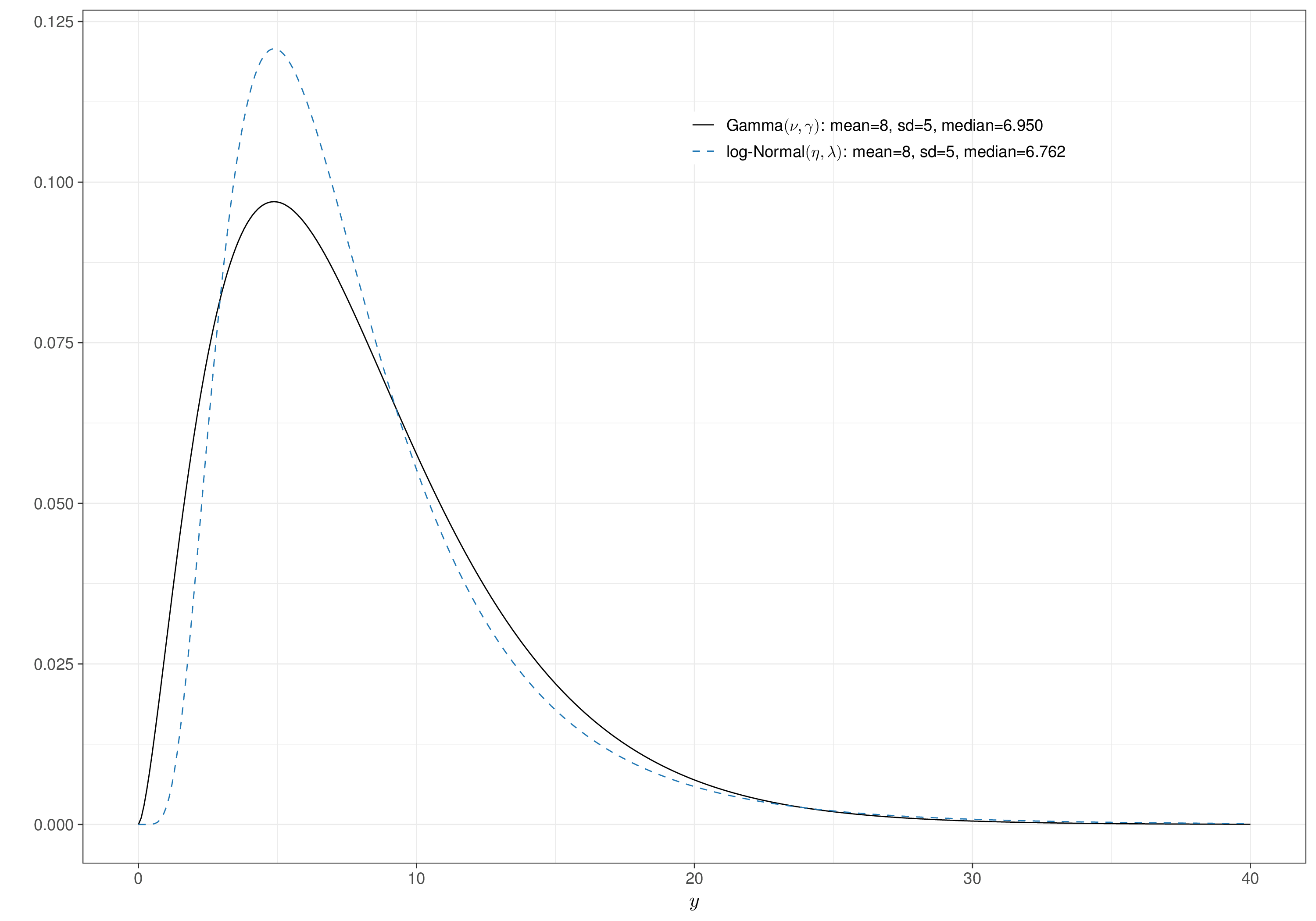
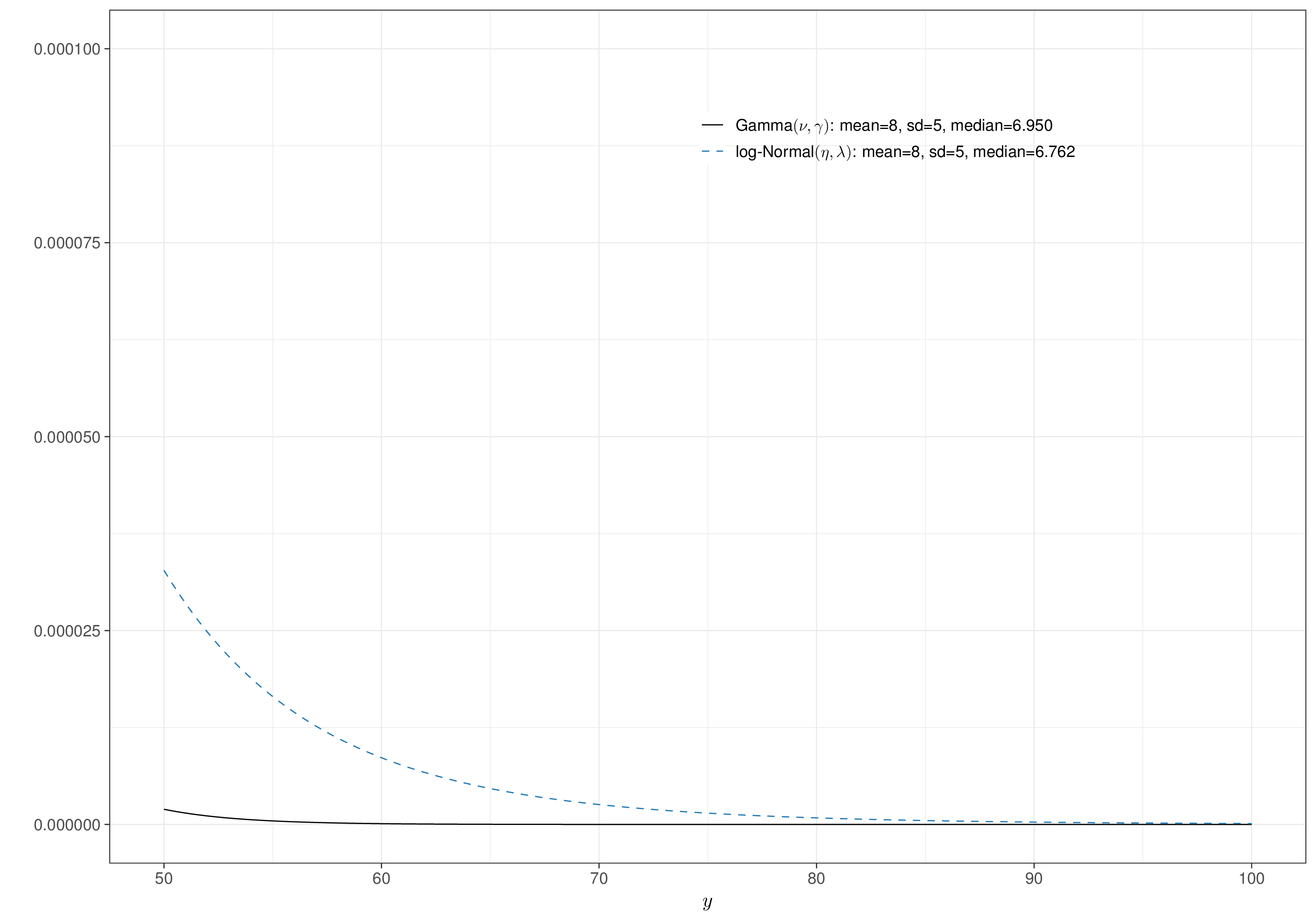
While the shape of the Gamma and log-Normal distribution tends to be superficially similar, there is an important difference. By the mathematical properties of the two distributions, the log-Normal tends to have much heavier tails, meaning that it tends to assign higher probability to very large values of the underlying variable, as is obvious in Figure 5.5 (b).

This may be seen as an attracting feature, in case we want to safeguard from the theoretically justified possibility of having very large values (e.g. for the cost associated with a given treatment), even without having observed any in the data.

Generally speaking, however, this often implies that the Gamma is a safer option to model variables such as costs, limiting the potential impact of too large ranges in the estimates (Thompson and Nixon, 2005).

When we can write down the algebraic relationships linking the natural-scale to the original-scale parameters analytically then posterior predictive Monte Carlo estimation is not necessary – given simulations for \((\eta,\lambda)\), we can simply rescale them properly and obtain simulations for the relevant parameter. For instance, to retrieve samples from the distribution of the natural scale variable \(y\) in the example above, we simply need to invert the relevant relationship in Equation 5.11 and compute \[\mu=\exp\left(\eta + \frac{1}{2}\lambda^2\right)\] directly using the output of our model.

Example 5.5. 10TT (continued): Gamma/Gamma MCF model – posterior predictive estimation. We can compute the estimates for the population average benefits using posterior predictive Monte Carlo simulation, using the following R code.

# Extracts the relevant parameters from the JAGS object 
nu.e=model$gg_mcf$BUGSoutput$sims.list$nu.e
mustar.e=model$gg_mcf$BUGSoutput$sims.list$mustar.e

# Compute the "average" rate 
rate=nu.e/mustar.e

# Posterior predictive estimation for the mean on the original scale
# 1. defines the number of MC simulations for the outcome
N=4000
# 2. defines the dimension of the object 'mu' in which to store the means
mu=matrix(NA,nrow=nrow(rate),ncol=2)
# 3. loops over the simulations for 'nu.e' and 'rate' 
for (i in 1:nrow(nu.e)) {
  for (t in 1:2) {
# Simulate 'mcsim' values of estar, for the current value of the parameters
    estar=rgamma(N,shape=nu.e[i,t],rate=rate[i,t])
# Computes the mean for the *inverse transformation*
    mu[i,t]=3-estar |> mean()
  }
}

# Computes the summary statistics
colnames(mu)=c("mu.e[1]","mu.e[2]")
mu |> bmhe::stats()

            mean         sd     2.5%   median    97.5%
mu.e[1] 1.584921 0.02156517 1.543266 1.584931 1.626938
mu.e[2] 1.566990 0.03320395 1.499450 1.567333 1.629637

As is possible to see, the posterior predictive version of this calculation aligns with the one provided directly in the JAGS model – but of course, in case of non-linear transformations for the outcomes, it would be necessary to either perform the back-transformation analytically, or by a similar numerical process as the one highlighted here.

5.3 Model selection

As shown throughout Section 5.2, there may be several formulations for our model, particularly in terms of “structural” assumptions, i.e. the way in which we describe both the sampling variability and the epistemic uncertainty about the model parameters. Sometimes, this is immaterial, because, at the end of the process, the inference is basically identical (just as in the case of the models in Examples 5.2 and 5.3). In general, however, the results will be sensitive to the structural choices and assumptions we make and thus it is natural to compare the performance of the models we have used, in order to select the “best” one.

Note 5.1: All models are wrong

In reality, we can never select the “best” model, at least not in absolute terms, as suggested by the famous statistical aphorism “All models are wrong but some are useful” (Box, 1979).

The deeper meaning of George Box’ quote is that the real aim of statistical modelling is not so much to find a hidden “truth”, but rather to update and, hopefully, reduce the uncertainty we have in our current understanding of complex phenomena, which we often struggle to even approximate to a reasonable degree.

Nonetheless, we can use statistical tools to assess the performance of competing model specifications, in order to narrow down even further our uncertainty and present results that are as consistent and robust as possible.

More importantly, we also note here that the idea presented in this section do not just apply to the case where ILD are available – assessing the impact of structural assumptions (e.g. using the tools described below) is an important part of any statistical modelling exercise and should be applied more widely.

5.3.1 Deviance Information Criterion (DIC)

One of the most popular tools to assess model fit and perform model selection in a Bayesian context is the Deviance Information Criterion (DIC, Spiegelhalter et al., 2002). The DIC is based on the model deviance, defined as \[D(\boldsymbol\theta)=-2\log \mathcal{L}(\boldsymbol\theta\mid\boldsymbol{y}). \tag{5.12}\] In isolation, a model’s deviance is meaningless, because the scale on which the likelihood is defined varies with different models and parameterisations – see Note 5.2 below. Thus, reporting the value of a single model’s deviance does not give information on its performance. Comparatively, however, it can be used to assess how well a given model fits the observed data, with respect to an alternative one. Models associated with a lower deviance fit the observed data better.

Similarly to other information criteria, e.g. the Akaike Information Criterion (AIC, Akaike, 1974) or the Bayesian Information Criterion (BIC, Schwarz, 1978), the DIC is designed to safeguard against the phenomenon of overfitting (which occurs when a model with a large number of parameters tends to do extremely well for the data at hand, but generally struggles to adapt to new/different data) by adding a penalty for model complexity.

Formally, in its original definition, the DIC is constructed as \[ \text{DIC}= \underbrace{\overline{D(\boldsymbol\theta)}}_{\text{"\texttt{dbar}"}} + p_D = \underbrace{D(\overline{\boldsymbol\theta})}_{\text{"\texttt{dhat}"}}+2p_D, \tag{5.13}\] where: \[\begin{align*} \overline{D(\boldsymbol\theta)}=\text{E}\left[D(\boldsymbol\theta)\right] & = \int -2\log\mathcal{L}(\boldsymbol\theta\mid\boldsymbol{y})p(\boldsymbol\theta\mid\boldsymbol{y})d\boldsymbol\theta \\ & \approx \frac{1}{S}\sum_{s=1}^S -2\log \mathcal{L}(\boldsymbol\theta^{(s)}) \end{align*}\] is the average model deviance (averaged over the posterior distribution of the model parameters, which can be approximated using a sample of \(S\) draws \(\boldsymbol\theta^{(1)},\ldots,\boldsymbol\theta^{(S)}\sim p(\boldsymbol\theta\mid \boldsymbol{y})\) obtained from the MCMC process); \[\begin{align*} D(\overline{\boldsymbol\theta})=D(\text{E}\left[\boldsymbol\theta\mid\boldsymbol{y}\right]) & = -2\log\mathcal{L}\left(\int \boldsymbol\theta p(\boldsymbol\theta\mid\boldsymbol{y})d\boldsymbol\theta \right) \\ & \approx -2\log \mathcal{L} \left( \frac{1}{S}\sum_{s=1}^S \boldsymbol\theta^{(s)} \right) \end{align*}\] is the model deviance calculated in correspondence of the average value of the model parameters (which, again, can be approximated using the simulations from the MCMC process); and \[p_D=\overline{D(\boldsymbol\theta)}-D(\overline{\boldsymbol\theta}) \tag{5.14}\] is the penalty for model complexity. This is the version used by BUGS when calculating the DIC – as evident by the note at the bottom of the outcome of the print(mbugs,...) instruction in Section 3.3. Equation 5.14 has an interesting direct interpretation as an estimate of the number of free parameters in the model, a quantity usually referred as “effective number of model parameters” – see Section 6.2 as well as Spiegelhalter et al. (2002) and Lunn et al. (2013) for more details on this, in the context of hierarchical models.

Note 5.2: Deviance and rescaled data

Technically, the dataset used to fit the two Normal/Normal models of Examples 5.2 and 5.3 is slightly different than the one used to fit the Gamma/Gamma MCF of Example 5.4; this is due to the rescaling applied to define \(e^*_i=3-e_i\).

Fortunately, in this case, we can rely on a combination of two factors: firstly, the underlying Normal sampling distribution is symmetric; and secondly, the transformation applied to the data is affine (i.e. a linear transformation that does not need to preserve the origin), which means that the shape of the likelihood function is unchanged.

To fix ideas, let us consider the simple case of one observation \(y\sim\text{Normal}(\mu,\sigma)\): using Equation 1.4, the likelihood function is \[ \mathcal{L}(\mu,\sigma\mid y) = \frac{1}{\sigma}\exp\left(-\frac{1}{2}\left(\frac{y-\mu}{\sigma}\right)^2\right) \] and thus the deviance is \[ D(\mu,\sigma) = -2\log\mathcal{L}(\mu,\sigma\mid y) = -2\left(-\log(\sigma) - \frac{1}{2}\left(\frac{y-\mu}{\sigma}\right)^2\right). \]

Using basic probability theory, we get that \(y^*=(3-y) \sim \text{Normal}(3-\mu,\sigma)=\text{Normal}(\mu^*,\sigma)\) and thus \[ \begin{aligned} D(\mu^*,\sigma) & = -2\log\mathcal{L}(\mu^*,\sigma\mid y^*) = -2\left(-\log \sigma - \frac{1}{2}\left(\frac{y^*-\mu^*}{\sigma}\right)^2\right)\\ & = -2\left(-\log\sigma - \frac{1}{2}\left(\frac{(3-y)-(3-\mu)}{\sigma}\right)^2\right) = D(\mu,\sigma). \end{aligned} \]

We could re-run the two Normal/Normal models on the exact same data (i.e. using \(e_i^*\) instead of \(e_i\), throughout), but while this would change the parameter estimates, it would not modify the computed value for the model deviance in the two Normal/Normal models and hence the DIC. Consequently, we can simply compare the three models using the DICs computed above and summarised in Table 5.3.

Notice however that other transformations or different distributional assumptions would break this property and thus comparing models based on different data would not be appropriate, in that case.

For instance, using standard probability theory, if \(y\sim\text{Gamma}(\text{shape}=\nu,\text{rate}=\gamma)\), then rescaling the data by a factor \(\kappa\) implies that \(y^*=y/\kappa \sim\text{Gamma}(\nu,\kappa\gamma)=\text{Gamma}(\nu,\gamma^*)\). Using Equation 1.3, we can derive the likelihood associated with the Gamma distribution and thus \[ D(\nu,\gamma) = -2\log\mathcal{L}(\nu,\gamma\mid y) = -2\left(\nu\log\gamma - \log\Gamma(\nu) + (\nu-1)\log y + \gamma y\right) \] but, substituting \(y^*=y/\kappa\) and \(\gamma^*=\kappa\gamma\) we obtain \[ \begin{aligned} D(\nu,\gamma^*) & = -2\log\mathcal{L}(\nu,\gamma^*\mid y^*) \\ & = -2\left(\nu\log\gamma - \log\Gamma(\nu) + (\nu-1)\log y + \gamma y - \log \kappa\right) \neq D(\nu,\gamma). \end{aligned} \]

In the general case with \(n\) observations, this implies that \(D(\nu,\gamma)=D(\nu,\gamma^*) + 2n\log\kappa\). Thus, even if in theory we could simply use the original scale cost data to apply the Gamma/Gamma model of Example 5.4, if we want to compare it with the two Normal models in Examples 5.2 and 5.3 by means of the DIC, we must use the same cost data in all three models, because rescaling by £1000 makes the deviance off by a factor of \(2n\log\kappa=2(167\log 1000) = 2307.19\) in the Gamma/Gamma model.

Despite its success and popularity in applied work, the DIC has been subject to substantial criticism – some of the main limitations are described in Plummer (2008), as well as in the extensive discussion of the original paper by Spiegelhalter et al. (2002).

Among these, one of the most cited is the fact that \(p_D\) (and hence the whole DIC) is, in general, not invariant to re-parameterisations of the model. To counter this issue, Gelman et al. (2013) suggest a slightly different definition for the penalty \[p_V=\frac{1}{2}\text{Var}\left[D(\boldsymbol\theta)\right], \tag{5.15}\] which has the advantage of being invariant to re-parameterisations of the model and non-negative. This is the version used by JAGS, as reported at the bottom of the output for the print(mjags,...) command in Section 3.3 as well as in the outputs of all print() commands in the examples above.

Note \(p_V\) vs \(p_D\)

Somewhat confusingly, earlier versions of the R2jags package still indicated the computed value for \(p_V\) with the general terminology pD. R2jags would highlight in the summary table produced by the print() method that the computation was performed using Equation 5.15, but the naming convention was still confusing.

This behaviour has changed in version 0.8-9 (released in October 2024), since which R2jags explicitly distinguishes between pV (the default calculation) and pD, which is computed using the method described by Plummer (2008) and using in the background the function rjags::dic.samples() – this is a slightly different version than the original one defined by Spiegelhalter et al. (2002), although it usually provides near-identical results.

Equation 5.14 has the obvious advantage of being extremely easy to compute, once the deviance is monitored. In addition, in the case of weak prior information, it also approximates the effective number of model parameters. When the prior is not dominated by the likelihood, however, this result does not hold and the penalty can vary in ranges that are more complex to analyse. This implies that the scale of the penalty and thus of the DIC may be different when using BUGS (i.e. \(p_D\)), as opposed to the default specification of JAGS based on \(p_V\).

5.3.2 Computing \(p_D\) manually

Irrespective of the software used to perform the MCMC analysis, we can still compute the penalty \(p_D\) by using the resulting simulations to estimate \(\overline{D(\boldsymbol\theta)}\) and \(D(\overline{\boldsymbol\theta})\).

The first one is easy to obtain as the mean of the simulated values for the deviance. For instance, considering the model in Example 5.4, this can be easily extracted from the JAGS object, as we show below.

As for \(D(\overline{\boldsymbol\theta})\), this is a bit more involved, because we first need to extract the mean value of all the model parameters and then compute the full likelihood function associated with these values.

In the case of the model in Example 5.4 this can be done using the following code. First we consider the part of the model that deals with the effects.

# 1. Model for the effects
# Extracts the shape parameter 
nu.e=c(
  model$gg_mcf$BUGSoutput$summary["nu.e[1]","mean"],
  model$gg_mcf$BUGSoutput$summary["nu.e[2]","mean"]
)
# Extracts the regression coefficients 
alpha0=model$gg_mcf$BUGSoutput$summary["alpha0","mean"]
alpha1=model$gg_mcf$BUGSoutput$summary["alpha1","mean"]
alpha2=model$gg_mcf$BUGSoutput$summary["alpha2","mean"]
# Computes the linear predictor
trt=data$Trt-1
u0=data$u0star
log.phi.e=alpha0 + alpha1*trt + alpha2*u0
# Computes the overall mean (needed for the costs)
mustar.e=numeric()
for (t in 1:2) {
  mustar.e[t]=exp(alpha0 + alpha1*(t-1))
}
# Computes the rate parameter
gamma.e=numeric()
for (i in 1:data$N) {
  gamma.e[i]=nu.e[data$Trt[i]]/exp(log.phi.e[i])
}
# Computes the likelihood contribution from each observation
lik.e=-2*dgamma(data$estar,shape=nu.e[data$Trt],rate=gamma.e,log=TRUE) 

The R code effectively replicates the constructions described for the JAGS model to use the mean value of the shape parameter nu.e and the linear predictor log.phi.e to derive the rate parameter gamma.e.

We then use the R built-in function dgamma() to compute the likelihood given the observed data data$estar and the shape and rate parameters computed at the average value. Note that this code computes the full likelihood, including any constant that does not depend on the parameters.

Technically, dgamma() returns the density of a Gamma distribution using Equation 1.2, given the value of the parameters. In the calculation here, however, we use always the same fixed (observed) data data$estar, but vary the parameters, thus constructing a likelihood, rather than a sampling distribution – and, incidentally, this is the same strategy used by BUGS when computing \(p_D\).

The option log=TRUE computes the likelihood on the log scale and by multiplying it by \(-2\) we obtain the individual contribution for the deviance with respect to the effects.

We can replicate this computation for the part of the model that deals with the costs, as in the code below.

# 2. Model for the costs
# Extracts the shape parameter 
nu.c=c(
  model$gg_mcf$BUGSoutput$summary["nu.c[1]","mean"],
  model$gg_mcf$BUGSoutput$summary["nu.c[2]","mean"]
)
# Extracts the regression coefficients 
beta0=model$gg_mcf$BUGSoutput$summary["beta0","mean"]
beta1=model$gg_mcf$BUGSoutput$summary["beta1","mean"]
beta2=model$gg_mcf$BUGSoutput$summary["beta2","mean"]
# Computes the linear predictor
log.phi.c=beta0 + beta1*(data$estar-mustar.e[data$Trt]) + beta2*(trt)
# Computes the rate parameter
gamma.c=numeric()
for (i in 1:data$N) {
  gamma.c[i]=nu.c[data$Trt[i]]/exp(log.phi.c[i])
}
# Computes the likelihood contribution from each observation
lik.c=-2*dgamma(data$c,shape=nu.c[data$Trt],rate=gamma.c,log=TRUE) 

The objects lik.e and lik.c are vectors of length 167 – one value for each individual in the data.

Once we have an estimate for these, we can simply sum them up to obtain an estimate for \(D(\overline{\boldsymbol\theta})\), which, in accordance with BUGS parlance, we indicate as dhat in the code below. Together with the estimate for \(\overline{D(\boldsymbol\theta)}\), indicated as dbar and obtained by simply extracting the average for the posterior distribution of the deviance, we can simply compute \(p_D\) and the DIC, according to Equations 5.14 and 5.13, using the code below.

# 3. Finally computes pD & DIC
# Computes the average model deviance
dbar=model$gg_mcf$BUGSoutput$summary["deviance","mean"]
# Computes the deviance at the average value for the parameters
dhat=sum(lik.e) + sum(lik.c)
# Computes pD
pD=dbar-dhat
# Computes DIC
DIC=dbar+pD

The computed values are \(p_D=-10.2\) and \(\text{DIC}=470\), which in this case are fairly similar to the estimates based on the calculation of \(p_V\), provided by JAGS (which can be found in the summary table in Example 5.4), although this is not necessarily always the case.

Note 5.3: Computing the likelihood using built-in JAGS functions

Of course, it is always possible to obtain the log-likelihood using the simulations for the model parameters and R commands, at the point of post-processing the output of the JAGS model.

However and conveniently, there is a built-in facility to generate a node that contains the individual contributions to the (log)likelihood, directly in the JAGS script.

For every distribution dxxxx that is available for sampling, JAGS has also a function logdensity.xxxx(), which takes as arguments the data and the relevant parameters to compute the resulting log-density, which in turns constitutes the full form of the likelihood function (see Note 1.3 in Section 1.2).

For example, if we consider a simple linear regression model, we can create the following JAGS code

model=function() {
  # Model for the data and linear predictor
  for (i in 1:n) {
    y[i] ~ dnorm(mu[i], tau)
    mu[i] <- X[i,] %*% beta
  # Computes the log-likelihood for the model
    log.lik[i] <- logdensity.norm(y[i], mu[i], tau)
  }
  # Prior distributions
  for (k in 1:K) {
    beta[k] ~ dnorm(0,0.001)
  }
  sigma ~ dexp(0.1)
  tau <- pow(sigma,-2)
}

to embed the basic assumptions and add a node log.lik[i], which, for each observation i automatically computes the individual contribution to the overall log-likelihood. We expand on this in Example 5.7.

While with a bit of coding and maths to obtain the relevant values for the deviance we can always post-process a JAGS object and obtain an estimate for \(p_D\), we do not necessarily need to do so and instead obtain an approximation to the value of \(p_D\) as would be computed by BUGS (and thus a more direct estimate of the number of effective parameters) using the function dic.samples() from the rjags package (which is automatically loaded when R2jags is). For instance, we can use code such as

rjags::dic.samples(object$model,n.iter=1000,type="pD")

where object is a R2jags object (e.g. mjags above) and n.iter is the number of iterations to be used to make the computation. When type=pD (which is the default), the element penalty in the output object is an approximation to \(p_D\).

In addition, since version 0.8-6, R2jags embeds this calculation in the call to the function jags(), where it is possible to specify an input pD=TRUE. If that is the case, then R2jags will first run the model and then dic.samples() to compute the penalty \(p_D\), which is stored in the resulting JAGS object, alongside the default \(p_V\), as we demonstrate in Example 5.6.

5.3.3 Using DIC to compare models

Technically speaking, a full-on, proper Bayesian analysis concerned with model selection would work by identifying a set of finite and exhausting models \(\mathcal{M}=(\mathcal{M}_1,\ldots,\mathcal{M}_H)\), where each of the models is indexed by a set of parameters \(\boldsymbol\theta\) and a suitable prior distribution \(p(\boldsymbol\theta\mid\mathcal{M}_h)\). In addition to this “standard” framework, we would add a prior distribution \(p(\mathcal{M}_h)\) for each of the alternative models – this would indicate the contextual assessment of model \(\mathcal{M}_h\) being the “true” one.

Under this framework, we would use the observed data \(\boldsymbol{y}\) and estimate \[ p(\mathcal{M}_h\mid \boldsymbol{y}) \propto p(\mathcal{M}_h) \int p(\boldsymbol{y}\mid \boldsymbol\theta,\mathcal{M}_h)p(\boldsymbol\theta\mid \mathcal{M}_h)d\boldsymbol\theta, \] which would then be used to compute a weighted average for any function of the parameters over the space of models.

While this approach is perfectly aligned with the Bayesian machinery, it has the important limitations of i) requiring that all possible models are completely specified and given a prior probability; and ii) that the set \(\mathcal{M}\) does include the “true” model. This is usually a very tall order – most of the times, we only have a very limited and far from exhaustive number of models that we can possibly use, which presents a major limitation to the fully-fledged Bayesian framework (see Lunn et al., 2013, sec. 8.3.3 for further discussion).

To overcome this issue, if we have two or more models based on the exact same data, we can use the DIC to provide a ranking and assess whether differences in model fit are “substantial” across the various models – notice that a meaningful comparison is not possible for models using different data, because, by definition, the likelihood function (which is conditional on the observed data) would be different – with the caveats discussed in Note 5.2, above.

Focussing on AIC, Burnham and Anderson (1998) propose a heuristic rule of thumb to compare models based on information criteria and Spiegelhalter et al. (2002) map this onto an evaluation based on DIC. Specifically, for a set of \(H\) competing models, we can compute the absolute difference in DIC between the \(h-\)th model and the one associated with the lowest DIC \[ \Delta\text{DIC}_h = \mid \min_h(\text{DIC}_h) - \text{DIC}_h \mid \tag{5.16}\] and then values for \(\Delta\text{DIC}_h<2\) indicate that model \(h\) deserves some consideration, while differences in the range [3–7] indicate less support towards model \(h\) and, in line with Burnham and Anderson (2002) discussion based on AIC, differences exceeding 10 indicate no support for the \(h-\)th model.

Example 5.6. 10TT (continued): model selection. Comparing the models in Example 5.2 and in Example 5.3 we can see from the summary tables that they have rather similar DIC values: 686 and 674, respectively. While the estimates are materially indistinguishable (as evident from Figure 5.4), according to the rule-of-thumb described above, the Normal/Normal MCF provides a much better fit to the data, as its DIC is over 10 points lower than that of the Normal/Normal independent model.

If we include in the mix the model in Example 5.4, the situation becomes even more clear-cut, as the DIC for the Gamma/Gamma MCF version is substantially lower, with a computed value of 493 – that is a difference of over 200 points with respect to the two versions of the Normal/Normal model, indicating a much better fit for the Gamma/Gamma MCF.

Especially in the absence of genuine information in the prior distributions, the computed value for \(p_V\) generally tends to agree with the value that could be obtained for \(p_D\). In this case, for Gamma/Gamma MCF model, \(p_V=12.4\), which is slightly higher than those for the Normal/Normal models, respectively obtained at 9 and 9.8. In this particular case, all the \(p_V\) values are reasonably aligned with the nominal number of fundamental parameters, which is 9 (alpha0, alpha1, alpha2, beta0, beta1, sigma.e[1], sigma.e[2], sigma.c[1] and sigma.c[2]) for the model in Example 5.2, 10 (with beta2 in addition to the ones above) for the model in Example 5.3 and 10 (alpha0, alpha1, alpha2, beta0, beta1, beta2, nu.e[1], nu.e[2], nu.c[1] and nu.c[2]) for the model in Example 5.4.

As mentioned above, more generally we can directly compute \(p_D\) from R2jags by adding the option pD=TRUE to the call to the function jags(). As all the models above have reached reasonable convergence, we can keep the other optional argument n.iter.pd to its default (1000 extra simulations) and re-run the three models. For instance, for the Normal/Normal independence model, the revised call to jags() would be as in the following code.

# Re-runs the model adding the option pD=TRUE
model$nn_indep=jags(
  data=data,
  parameters.to.save=c(
    "mu.e","mu.c","alpha0","alpha1","alpha2","beta0","beta1","sigma.e","sigma.c"
  ),
  inits=NULL,n.chains=2,n.iter=5000,n.burnin=3000,n.thin=1,DIC=TRUE,
  # This specifies the model code as the function nn_indep()
  model.file=nn_indep,
  # Adds the computation for pD
  pD=TRUE
)

# Shows the summary table, including the estimate for pD
print(model$nn_indep,digits=3,interval=c(0.025,0.5,0.975))

Inference for Bugs model at "/tmp/RtmpbIPSKN/modelff8ab4e104790.txt", 
 2 chains, each with 5000 iterations (first 3000 discarded)
 n.sims = 4000 iterations saved. Running time = 0.67 secs
            mu.vect sd.vect     2.5%      50%    97.5%  Rhat n.eff
alpha0        1.551   0.021    1.511    1.552    1.591 1.002  1100
alpha1       -0.006   0.039   -0.081   -0.006    0.072 1.001  4000
alpha2        1.277   0.072    1.133    1.278    1.418 1.001  4000
beta0         1.556   0.136    1.298    1.556    1.823 1.001  4000
beta1         1.092   0.429    0.255    1.089    1.919 1.001  4000
mu.c[1]    1556.303 135.586 1298.248 1555.970 1822.789 1.001  4000
mu.c[2]    2647.949 408.872 1855.692 2647.651 3440.929 1.001  4000
mu.e[1]       1.551   0.021    1.511    1.552    1.591 1.002  1100
mu.e[2]       1.545   0.033    1.480    1.545    1.610 1.001  4000
sigma.c[1]    1.354   0.101    1.173    1.348    1.566 1.001  4000
sigma.c[2]    3.323   0.289    2.800    3.306    3.921 1.001  4000
sigma.e[1]    0.208   0.015    0.181    0.207    0.239 1.004   460
sigma.e[2]    0.267   0.024    0.226    0.266    0.317 1.001  4000
deviance    676.771   4.284  670.450  676.079  686.917 1.001  4000

For each parameter, n.eff is a crude measure of effective sample size,
and Rhat is the potential scale reduction factor (at convergence, Rhat=1).

DIC info (using the rule: pV = var(deviance)/2)
pV = 9.2 and DIC = 686.0
DIC info (using the rule: pD = Dbar-Dhat, computed via 'rjags::dic.samples')
pD = 9.1 and DIC = 685.8
DIC is an estimate of expected predictive error (lower deviance is better).

The summary table now includes at the bottom the values for \(p_D\) and the revised DIC – notice that, because JAGS needs to re-runs the model to compute \(p_D\), the DIC associated with it is computed based on a new (possibly slightly different) distribution of the deviance, although if the model is at convergence, the discrepancy is minimal. For the same reason, the reported values for \(p_V\) and DIC are also slightly different to the ones in Example 5.2, but these differences are only down to Monte Carlo error (due to the new MCMC run used to construct this table).

Table 5.3: Model selection via DIC, using the two versions – the first one based on \(p_V\) and the second based on \(p_D\). The values reported for \(p_V\) are those obtained in Examples 5.2, 5.3 and 5.4, based on the original model runs

Model	\(p_V\)	\(\text{DIC}=p_V+\overline{D(\boldsymbol\theta)}\)	\(p_D\)	\(\text{DIC}=p_D+\overline{D(\boldsymbol\theta)}\)
Normal/Normal independent	8.95	686	9.14	686
Normal/Normal MCF	9.83	674	10.56	675
Gamma/Gamma MCF	12.39	493	10.68	491

We can do the same for all three models considered here. The resulting values for the model fitting statistics are presented in Table 5.3. As mentioned above, the Normal/Normal independent model is the one with the worst performance, according to the DIC, with values that are over 10 points higher than for the Normal/Normal MCF and almost 200 points above the Gamma/Gamma MCF, confirming its better performance over the others. For the Gamma/Gamma MCF, the value computed by R2jags::jags() is also close (but not identical, again due to simulation error) to the one we obtained manually in Section 5.3.2.

NoteWhat if?…

Incidentally, if we included some substantial information in the prior for the shape of the effects, in the Gamma/Gamma MCF model of Example 5.4, e.g. \(\nu_{et}\sim\text{Exponential}(6)\), to encode the assumption that \(\Pr(\nu_{et}>0.5)\approx 0.05\), then we would get estimates for the DIC of 795, for \(p_V\) of 129 and for \(p_D\) of 10.3.

Because of the gross mis-specification for the shape parameter, not only would this change the scale of the estimate for \(p_V\), but also the ordering of the three models – this new version of the Gamma/Gamma MCF would have worse performance than the two Normal/Normal models!

5.3.4 Other information criteria

As mentioned above, the DIC is not the only (or necessarily the best) way of assessing model fitting and, in fact, several alternatives have been proposed; Gelman et al. (2013, ch. 7) present a few, including the Watanabe Applicable Information criterion (WAIC), as well as procedures such as leave-one-out cross validation (LOO-CV), which are perhaps considered more “modern” measures of predictive accuracy. These are similar to DIC as they use a penalty to discount a measure of model fit. However, instead of directly on the likelihood, they are based on the posterior predictive distribution, given the observed data.

Formally, for each observation \(i=1,\ldots,n\), we define the log pointwise predictive density (lpd) as \[ \begin{aligned} \text{lpd} & = \sum_{i=1}^n \log p(y_i \mid \boldsymbol{y}) = \sum_{i=1}^n \log \int p(y_i\mid\boldsymbol\theta)p(\boldsymbol\theta\mid\boldsymbol{y})d\boldsymbol\theta \\ & = \sum_{i=1}^n \log \text{E}_{\boldsymbol\theta\mid\boldsymbol{y}}\left[p(y_i\mid\boldsymbol\theta)\right] \\ & \approx \sum_{1=1}^n \log \frac{1}{S}\sum_{s=1}^S p\left(y_i \mid \boldsymbol\theta^{(s)}\right) \end{aligned} \] and \[ \text{WAIC}= -2\text{lpd} + 2p_W, \] where \(p_W\) is the penalty. There are different choices for the definition of \(p_W\), but a simple and effective one is to consider \[ \begin{aligned} p_W & = \sum_{i=1}^n \text{Var}_{\boldsymbol\theta\mid\boldsymbol{y}}\left[\log p(y_i\mid\boldsymbol\theta) \right] \\ & \approx \sum_{i=1}^n \frac{1}{S-1} \sum_{s=1}^S \left[ \log p\left(y_i\mid \boldsymbol\theta^{(s)}\right) - \frac{1}{S}\sum_{s=1}^S \log p\left(y_i\mid\boldsymbol\theta^{(s)}\right) \right]^2. \end{aligned} \tag{5.17}\] The penalty can be interpreted similarly to \(p_D\), as a measure of “effective number of parameters”.

These computations are implemented in the R package loo (Vehtari et al., 2024), which can be used to compute the \(\text{WAIC}\), as well as the LOO-CV, which is an estimate of out-of-sample predictive, where the lpd is modified to consider \(\log p(y_i\mid\boldsymbol{y}_{-i})\). More details are presented in Vehtari et al. (2017) and Gelman et al. (2013).

Example 5.7. Computing the WAIC using the loo package. We can slightly modify the Gamma/Gamma MCF model to include the computation of the individual log-likelihood contribution, which we can then use to compute WAIC and LOO. As discussed in Note 5.3 above, it is sufficient to add a single command to the model code function defined in Example 5.4

gg_mcf_waic=function(){
  for (i in 1:N) {
    ...
   # Computes the individual contributions to the log-likelihood
   log.lik[i] <- logdensity.gamma(estar[i], nu.e[Trt[i]], gamma.e[Trt[i],i]) + 
                 logdensity.gamma(c[i], nu.c[Trt[i]], gamma.c[Trt[i],i])
  }
  ...
}

to include a node log.lik[i], which sums the contributions to the likelihood from both cost and effects data. We can run the model, e.g. using the following R code

m_waic=jags(
  data=data,parameters.to.save=c("log.lik"),model.file=gg_mcf_waic,
  inits=NULL,n.chains=2,n.iter=5000, n.burnin=3000,n.thin=1,DIC=TRUE
)

and then use the simulated values for the node log.lik (which consist of n.sims=4000 simulations for each of the 167 individual observations) to feed into the loo functions and compute the WAIC, for example as in the following R code.

# Prints the WAIC
loo::waic(m_waic$BUGSoutput$sims.list$log.lik)

Computed from 4000 by 167 log-likelihood matrix.

          Estimate   SE
elpd_waic   -245.4 21.3
p_waic        10.3  1.4
waic         490.8 42.5

2 (1.2%) p_waic estimates greater than 0.4. We recommend trying loo instead. 

The first quantity returned by this function is an estimate of the expected log pointwise predictive density, defined as \[ \text{elpd} = \text{E}_{Y_i}\left[\sum_{i=1}^n \log p(y_i\mid \boldsymbol{y})\right] = \sum_{i=1}^n \int \tilde{p}(y_i)\log p(y_i \mid \boldsymbol{y})dy_i, \] where \(\tilde{p}(\cdot)\) is the unknown distribution representing the “true” data-generating process for an observation \(y_i\). The elpd is a measure of predictive accuracy for the \(n\) data points, taken one at a time and is estimated as \(\widehat{\text{elpd}}=\text{lpd}-p_W\); this is the quantity labelled as elpd_waic, above.

The computed value for the \(\text{WAIC}\) and \(p_W\) are fairly close to the ones obtained using DIC and \(p_D\) (see Table 5.3). In this particular case, loo() returns a warning: as is obvious by Equation 5.17, the penalty is computed by summing over all the individual \(n\) contributions and the fact that for some observations \(p_W\) exceeds the arbitrarily chosen threshold of 0.4 may pose some concerns around the reliability in the overall estimate (see Vehtari et al., 2017 for more details on diagnostics for the WAIC).

For this reason, loo() suggests moving to the more robust LOO-CV approach, which we can obtain using the following R commands.

# Prints the LOO-CV
loo::loo(m_waic$BUGSoutput$sims.list$log.lik)

Computed from 4000 by 167 log-likelihood matrix.

         Estimate   SE
elpd_loo   -245.4 21.3
p_loo        10.4  1.4
looic       490.9 42.6
------
MCSE of elpd_loo is 0.1.
MCSE and ESS estimates assume independent draws (r_eff=1).

All Pareto k estimates are good (k < 0.7).
See help('pareto-k-diagnostic') for details.

The estimates are effectively identical and in fact, the LOO suggests that the estimates are consistent (see Vehtari et al., 2017 for more details on how Pareto smoothed importance sampling is used to improve the efficiency of the LOO estimate).

5.3.5 Model averaging

One possible way to reconcile the uncertainty over distributional assumptions (cfr. also the discussion in Section 4.3.4) is to consider a form of “model averaging”. Here, instead of simply presenting a measure of model fitting with a view to selecting the “best” option (as in Table 5.3), the idea is to instead use the model fitting statistics to derive weights and then construct a “meta-model”, which combines the feature of all the options being considered.

Expanding on a suggestion based on AIC in Burnham and Anderson (2002), as well as related work in Jackson et al. (2009), Baio (2012) proposes to weigh each of the \(H\) competing models using weights determined as \[ w_h=\frac{\exp(-0.5\Delta\text{DIC}_h)}{\sum_{h=1}^H \exp(-0.5\Delta\text{DIC}_h)}, \tag{5.18}\] with \(\Delta\text{DIC}_h\) defined in Equation 5.16.

The underlying implication is that the weight for the \(h-\)th model decreases steeply with the increase in the absolute difference between its DIC and the one associated with the minimum DIC – and effectively vanishes to 0 as \(\Delta\text{DIC}_h\) approaches 10, as shown in Figure 5.6 (in the case of two models being compared) and in line with Section 5.3.3.

Figure 5.6: The relationship between a model weight and its absolute difference with the model associated with the lowest DIC, assuming these are the only models under consideration.

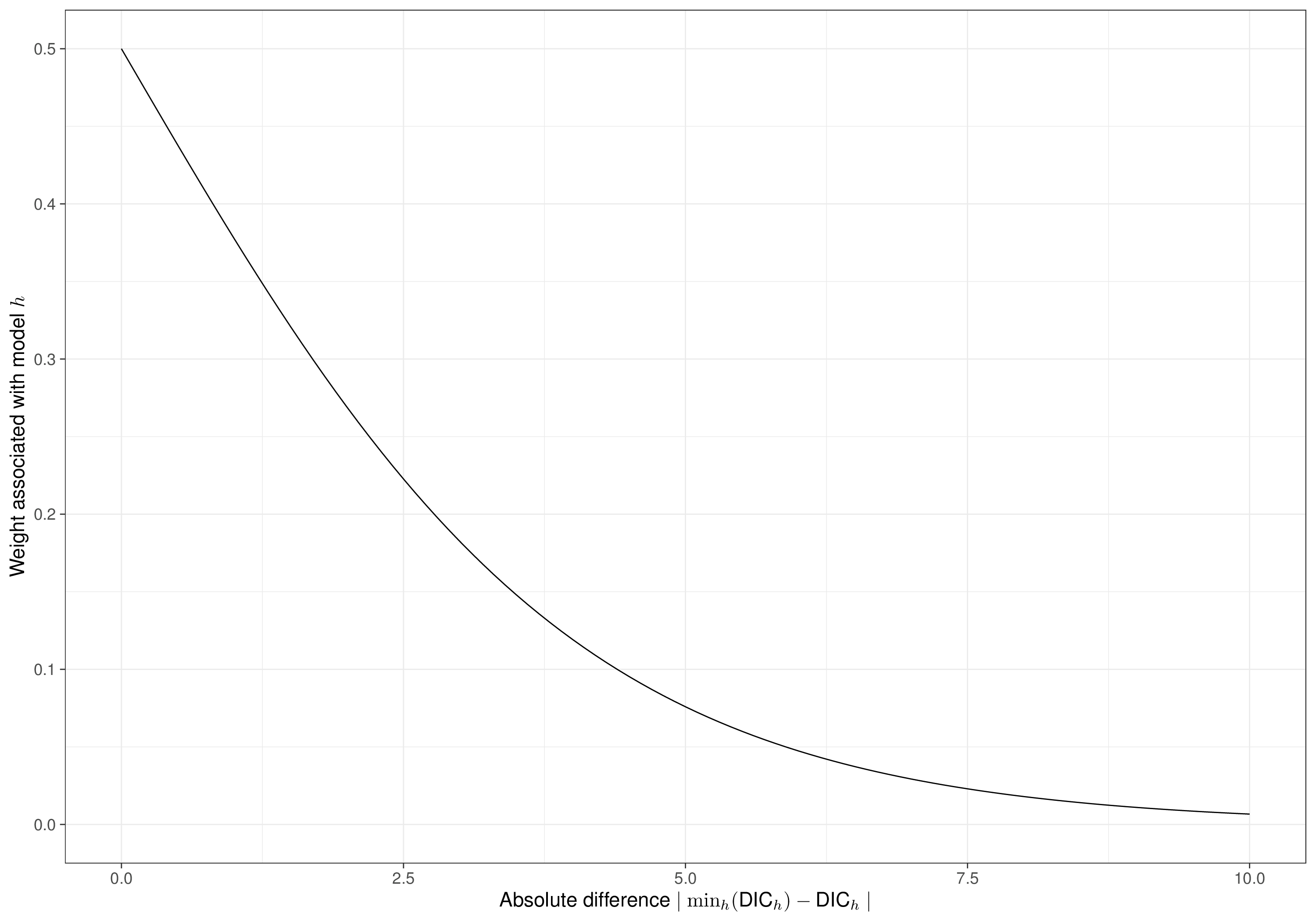
In order to construct the model average, we can simply multiply the MCMC simulations for the main parameters or computed quantities of interest for each of the \(H\) models being considered by the respective weights in Equation 5.18. We demonstrate this computation in Example 5.6. Note that the analysis in Figure 5.6 suggests that constructing the model average is only useful if there is substantial uncertainty among at least two of the \(H\) options, because otherwise the weights will be very small and thus the model average will be almost entirely driven by the best fitting model (for example as in Example 5.6).

5.4 Cost-effectiveness modelling

As discussed in Chapter 4, the statistical model is the most fundamental building block for the process of HTA, but once we have the estimates for the relevant parameters, we still need to post-process them to propagate the underlying uncertainty all the way to the decision process.

In the context of ILD and especially in the case of HTA alongside trial data, the model parameters are very close to the actual economic quantities, necessary for the HTA evaluation – typically we retrieve directly full estimates for the population average benefit and costs, in each treatment arm and these are simply combined to obtain the quantities \((\Delta_e,\Delta_c)\), upon which we base the decision making, e.g. by computing summary measures such as the ICER and EIB, as well as performing the uncertainty analysis, as detailed in Chapter 4.

Example 5.8. 10TT (continued): cost-effectiveness analysis. We can post-process the outcome by accessing directly the simulations from the BUGS model, for instance stored in the object model$sims.list. For instance, we could construct the relevant variables \((\Delta_e,\Delta_c)\) as

delta_e=model$nn_indep$BUGSoutput$sims.list$mu.e[,2]-
  model$BUGSoutput$sims.list$mu.e[,1]
delta_c=model$nn_indep$BUGSoutput$sims.list$mu.c[,2]-
  model$BUGSoutput$sims.list$mu.c[,1]

and then we could use these to, for instance, plot the Cost-Effectiveness plane.

Alternatively (and, perhaps, more efficiently), we can use the R package BCEA (Baio et al., 2025). This is a rather simple package, really, which codes up a set of operations to be performed on objects given as input by the user, representing simulations from the distribution of the population average cost and benefits².

This means we would only need to feed the simulations to the function bcea() to then produce a range of standardised output for the economic evaluation. For instance, we could use the following R code.

# Load 'BCEA'
library(BCEA)
# Defines a list of labels for the interventions
interventions=c("Standard","Active intervention")
# Sets the reference (t=2=intensive case management)
ref=2

# 1. Normal/Normal independent
# Defines the variables for effects and costs
eff=model$nn_indep$BUGSoutput$sims.list$mu.e
cost=model$nn_indep$BUGSoutput$sims.list$mu.c
# Runs BCEA  
m_nn_indep=bcea(
  eff=eff,cost=cost,interventions=interventions,ref=ref
)

# 2. Normal/Normal MCF
# Defines the variables for effects and costs
eff=model$nn_mcf$BUGSoutput$sims.list$mu.e
cost=model$nn_mcf$BUGSoutput$sims.list$mu.c
# Runs BCEA
m_nn_mcf=bcea(
  eff=eff,cost=cost,interventions=interventions,ref=ref
)

# 3. Gamma/Gamma MCF
# Defines the variables for effects and costs
eff=model$gg_mcf$BUGSoutput$sims.list$mu.e
cost=model$gg_mcf$BUGSoutput$sims.list$mu.c
# Runs BCEA
m_gg_mcf=bcea(
  eff=eff,cost=cost,interventions=interventions,ref=ref
)

Figure 5.7 shows the cost-effectiveness plane with overlaid a contour for the joint posterior distribution of \((\Delta_e,\Delta_c)\) – these figures can be obtained using the contour2() function from BCEA.

(a)

 

(b)

 

(c)

 

Figure 5.7: The contour plot overlaid on the cost-effectiveness plane. Panel (a) shows the cost-effectiveness plane for the Normal/Normal independent model, while panel (b) presents the results for the Normal/Normal MCF. The two are virtually identical. Panel (c) shows a different picture and interpretation, for the Gamma/Gamma MCF model.

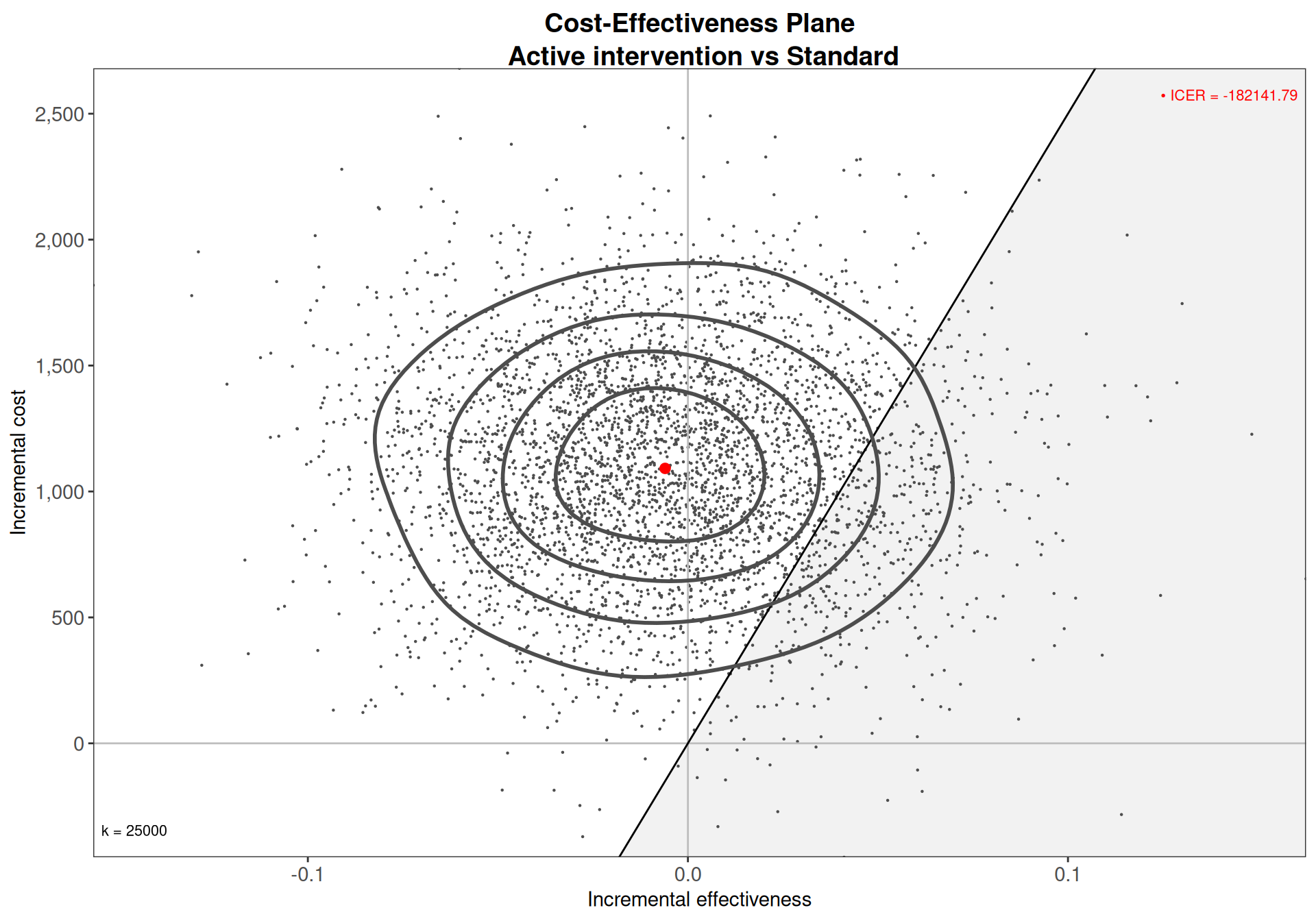
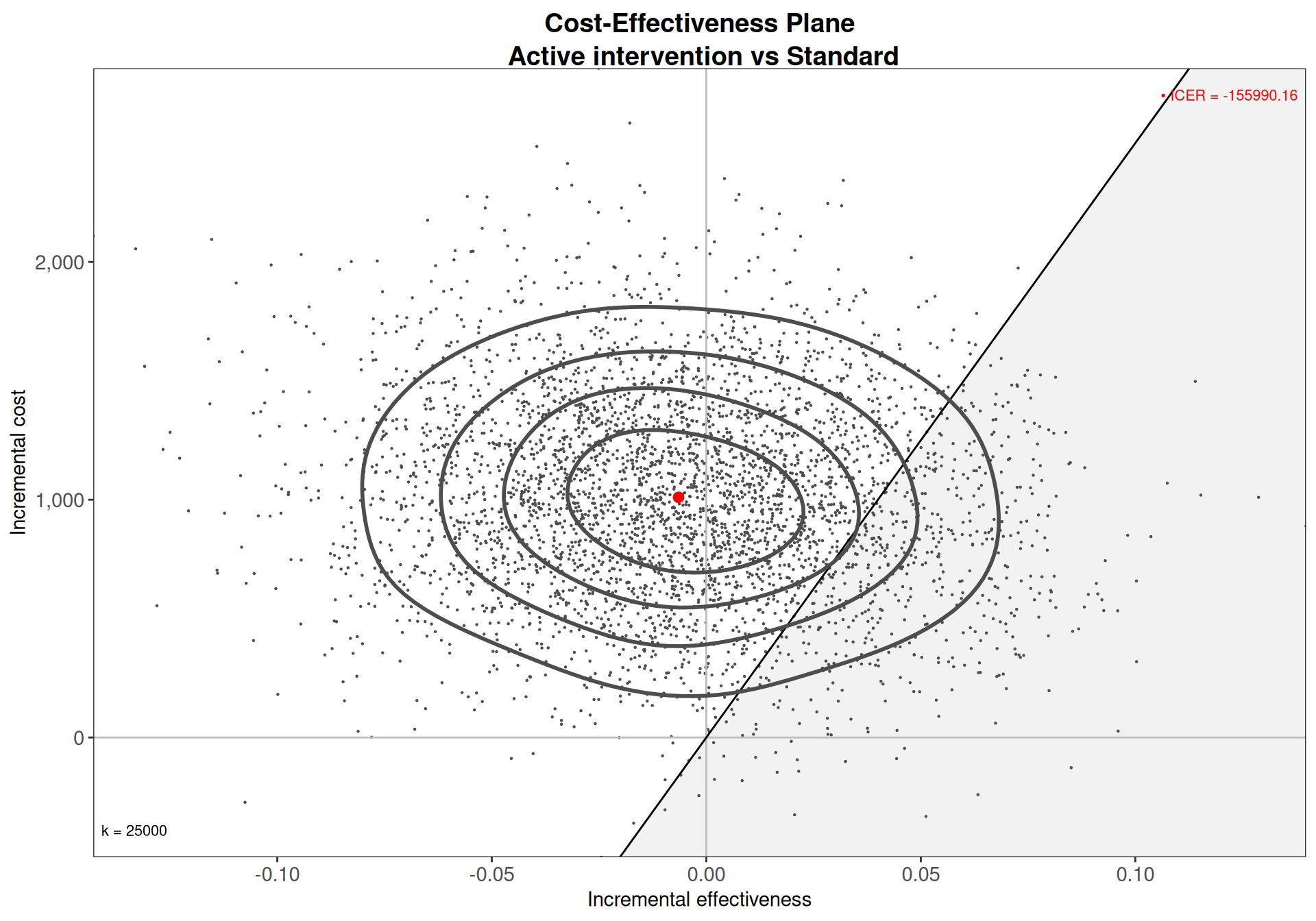
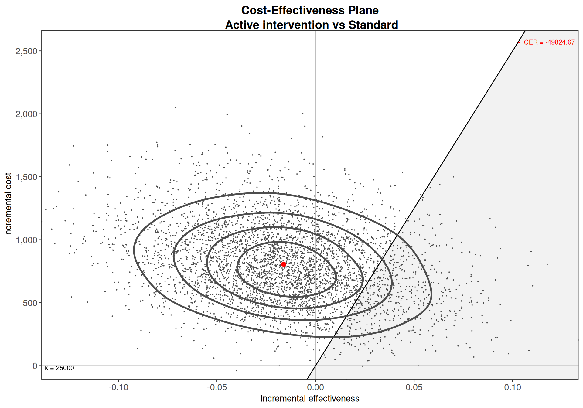
As is possible to see (and consistently with the discussion detailed throughout this chapter), the two Normal/Normal models of Examples 5.2 and 5.3 provide similar results. Figures 5.7 (a) and 5.7 (b) show more or less the same picture, with the larger dot in the middle of the contour representing the ICER that, albeit numerically slightly different, is firmly placed outside the “sustainability area”. In both cases, we would conclude that the intervention is not cost-effective, for the default threshold of £25 000 per QALY, although there seems to be some uncertainty, based on the proportion of points that lay below the cost-effectiveness threshold line. As for the Gamma/Gamma MCF, this result is generally confirmed, while the ICER is numerically different.

These results are even more obvious when looking at the CEACs displayed in Figure 5.8 and obtained using the BCEA function ceac.plot(). Generally speaking, when a BCEA object is constructed through the call to the function bcea(), as shown above, then it is possible to apply various plotting and summary methods by simply using it as the main parameter for a given function. For instance, the command ceac.plot(m_nn_indep) plots the CEAC for the Normal/Normal independent model.

More importantly, if in the call to any BCEA plotting method we specify the option graph=gg (= ggplot) for the graphical engine, then the resulting objects can be manipulated further, taking advantage of the ggplot2 capabilities. For instance, Figure 5.8 is obtained using the following code.

# Plots the CEAC with the 'ggplot' graphical engine and saves the graphs to the
# R objects 'p1', 'p2' and 'p3'
p1=ceac.plot(m_nn_indep,graph="gg")
p2=ceac.plot(m_nn_mcf,graph="gg")
p3=ceac.plot(m_gg_mcf,graph="gg")

# Post-processes the graphs to superimpose the three CEACs
# First stack the underlying data (extracted from the three 'ggplot' objects)
# And associate each with a 'model' variable
p1$data |> mutate(model="Normal/Normal indep") |>
  bind_rows(p2$data |> mutate(model="Normal/Normal MCF")) |>
  bind_rows(p3$data |> mutate(model="Gamma/Gamma MCF")) |> 
# Then use 'ggplot' to make the actual plot using the three original datasets
# but different colours for each model
  ggplot(aes(k,ceac,color=model)) + geom_line() +
# And then provide further customisation
  xlab("Willingness to pay") + ylim(0,1) +
  ylab("Probability of cost effectiveness") + 
  labs(title="Cost Effectiveness Acceptability Curves",color="Model") +
  theme(
    legend.position="inside",legend.position.inside=c(.6,.75),
    legend.background=element_blank()
  ) + scale_color_manual(values=c("#000000","#1F77B4","#FF7F0E"))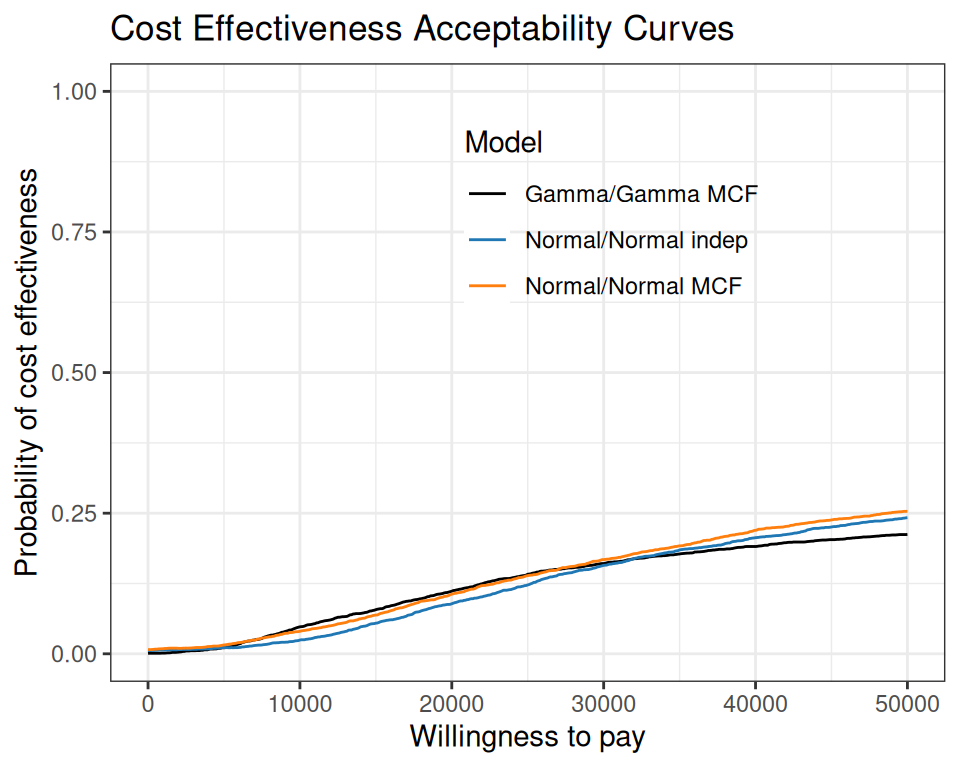 

Figure 5.8: The Cost-Effectiveness Acceptability Curves for the three models described in the chapter.

All CEACs in Figure 5.8 have consistently a low value (well below 0.5), which is only relatively sensitive to the choice of the willingness to pay threshold along the \(x\)–axis, indicating that, in this particular occasion, there is clear evidence (and little uncertainty) about the fact that, conditionally on the model assumptions, the new intervention is not cost-effective.

The optimal decision is then to keep the standard of care, which can also be assessed using the summary() method from BCEA. For instance, when applied to the Gamma/Gamma MCF model, this would return the following output.

summary(m_gg_mcf)

Cost-effectiveness analysis summary 

Reference intervention:  Active intervention
Comparator intervention: Standard

Standard dominates for all k in [0 - 50000] 


Analysis for willingness to pay parameter k = 25000

                    Expected net benefit
Standard                           38084
Active intervention                36873

                                    EIB   CEAC   ICER
Active intervention vs Standard -1211.5 0.1415 -49825

Optimal intervention (max expected net benefit) for k = 25000: Standard
          
EVPI 80.27

We can also use the models simulations to perform a structural uncertainty analysis, combining them into a “model average”, based on weights determined by the respective DICs, as described in Section 5.3.5. We could do this manually, first constructing the weights according to Equation 5.18, then multiplying them by the objects eff and cost for each of the three alternative models and finally adding the results together and feeding them to BCEA, to obtain the model average output, say m_avg.

More simply, we can use the BCEA function struct.psa(), which runs exactly these operations in the background.

# Defines a list with the simulations for the effects
effects=list(
  model$nn_indep$BUGSoutput$sims.list$mu.e,
  model$nn_mcf$BUGSoutput$sims.list$mu.e,
  model$gg_mcf$BUGSoutput$sims.list$mu.e
)
# Defines a list with the simulations for the costs
costs=list(
  model$nn_indep$BUGSoutput$sims.list$mu.c,
  model$nn_mcf$BUGSoutput$sims.list$mu.c,
  model$gg_mcf$BUGSoutput$sims.list$mu.c
)
# Defines a list of models
models=list(
  "nn-indep"=model$nn_indep,"nn-mcf"=model$nn_mcf,"gg-mcf"=model$gg_mcf
)

# Finally runs struct.psa to compute the model average
m_avg=struct.psa(
  models,effects,costs,ref=ref,interventions=interventions
)

The object m_avg is for all intents and purposes similar to the various BCEA objects created above (and, in fact, it also is in the class bcea, which means that it can access all the same methods and functions as the three BCEA fits above). In addition, however, it also contains a few more outputs (and the additional class struct.psa).

We can visualise the weights associated with each of the three models considered using the following command.

# Shows the weights for each of the three models, in the order with which 
# we have passed them in the 'models' list
m_avg$w

    nn-indep       nn-mcf       gg-mcf 
1.587980e-42 4.859974e-40 1.000000e+00 

Unsurprisingly, here the third model dominates, with a weight of effectively 1. This is of course consistent with Figure 5.6 and Table 5.3: we already know that the Gamma/Gamma MCF is way superior in terms of model fitting, as assessed by the DIC. We can check this also by creating the summary for the model average,

summary(m_avg)

Cost-effectiveness analysis summary 

Reference intervention:  Active intervention
Comparator intervention: Standard

Standard dominates for all k in [0 - 50000] 


Analysis for willingness to pay parameter k = 25000

                    Expected net benefit
Standard                           38084
Active intervention                36873

                                    EIB   CEAC   ICER
Active intervention vs Standard -1211.5 0.1415 -49825

Optimal intervention (max expected net benefit) for k = 25000: Standard
          
EVPI 80.27

which looks identical to the one produced above for the Gamma/Gamma MCF alone. Of course, in cases where competing models based on the same data showed closer fit, the model average would be a mixture of its individual components and would be much more worthy of reporting.

5.5 Conclusions

This chapter has focused on the analysis of individual-level data, e.g. coming from HTA alongside a RCT. We have discussed the “standard” framework of analysis, often based on unrealistic simplifying assumptions, such as independence between costs and benefits and underlying Normality. We have also showed how a Bayesian approach is able to naturally and relatively simply relax these assumptions, especially through the “Marginal/Conditional” factorisation.

We have also considered various other important aspects of ILD modelling, including assessement of model fitting and its use to make model selection choices. We have also explored suitable measures such as the DIC, which will also be used later in the book.

In the next chapter, we present a different background for HTA modelling, in which the data do not provide information at the individual-level, but rather are obtained using summary statistics, perhaps coming from systematic literature review.

Akaike, H., 1974. A new look at the statistical model identification. IEEE Transactions on Automatic Control 19, 716–723.

Baio, G., 2012. Bayesian Methods in Health Economics. CRC Press, Boca Raton, FL.

Baio, G., Heath, A., Berardi, A., Green, N., 2025. Bayesian Cost-Effectiveness Analysis with the R Package BCEA, 2nd ed. Springer.

Beeken, R., Leurent, B., Vickerstaff, V., Wilson, R., Croker, H., Morris, S., et al., 2017. A brief intervention for weight control based on habit-formation theory delivered through primary care: results from a randomised controlled trial. International Journal of Obesity 41, 246–254.

Box, G., 1979. Robustness in the strategy of scientific model building, in: Robustness in Statistics. Elsevier, pp. 201–236.

Burnham, K., Anderson, D., 2002. Model Selection and Multimodel Inference, 2nd ed. Springer.

Burnham, K., Anderson, D., 1998. Model Selection and Inference. Springer.

Gabrio, A., Mason, A., Leurent, B., Gomes, G., 2025. Missing Data, in: Baio, G., Thom, H., Pechivanoglou, P. (Eds), R for Health Technology Assessment. Chapman and Hall/CRC.

Gelman, A., Carlin, J.B., Stern, H.S., Dunson, D., Vehtari, A., Rubin, D., 2013. Bayesian Data Analysis, 3rd ed. Chapman and Hall/CRC, New York, NY.

Jackson, C.H., Thompson, S.G., Sharples, L.D., 2009. Accounting for uncertainty in health economic decision models by using model averaging. Journal of the Royal Statistical Society: Series A 172, 383–404.

Keng, M.J., Schlackow, I., Pullenayegum, E., 2025. Individual level data, in: Baio, G., Thom, H., Pechivanoglou, P. (Eds), R for Health Technology Assessment. Chapman and Hall/CRC.

Lunn, D., Jackson, C., Best, N., Thomas, A., Spiegelhalter, D., 2013. The BUGS Book. Chapman and Hall/CRC.

National Institute for Health and Care Excellence [NICE], 2016. The Social Care Guidance Manual. URL https://www.nice.org.uk/process/pmg10

O’Mahony, J., Paulden, M., 2014. NICE’s selective application of differential discounting: ambiguous, inconsistent, and unjustified. Value in Health 17, 493–496.

Plummer, M., 2008. Penalized loss functions for Bayesian model comparison. Biostatistics 9, 523–539.

Schwarz, G., 1978. Estimating the dimension of a model. The Annals of Statistics 461–464.

Spiegelhalter, D., Best, N., Carlin, B., Van Der Linde, A., 2002. Bayesian measures of model complexity and fit. Journal of the Royal Statistical Society: Series B 64, 583–639.

Thompson, S., Nixon, R., 2005. How sensitive are cost-effectiveness analysis to choice of parametric distributions? Medical Decision Making 14, 421–428.

Vehtari, A., Gabry, J., Magnusson, M., Yao, Y., Bürkner, P., Paananen, T., et al., 2024. loo: Efficient leave-one-out cross-validation and WAIC for Bayesian models. URL https://mc-stan.org/loo/

Vehtari, A., Gelman, A., Gabry, J., 2017. Practical Bayesian model evaluation using leave-one-out cross-validation and WAIC. Statistics and Computing 27, 1413–1432.

Willan, A., Briggs, A., 2006. The Statistical Analysis of Cost-effectiveness Data. John Wiley and Sons, Chichester, UK.

Zellner, A., 1962. An efficient method of estimating seemingly unrelated regressions and tests for aggregation bias. Journal of the American Statistical Association 57, 348–368.

---

1. Unsurprisingly, the author does prefer to speak Statistics.

2. In reality, as far as BCEA is concerned, the inputs do not have to come from a full Bayesian analysis and thus represent samples from the joint posterior distributions. As long as simulations are provided (e.g. from a bootstrap procedure, in a frequentist approach), the user can call the main BCEA function and obtain the post-processed results. BCEA will silently judge the user, in that case, though.