| Placebo | Magnesium | |||||
|---|---|---|---|---|---|---|
| ID | Name | Year | Deaths \((r_1)\) | Total \((n_1)\) | Deaths \((r_2)\) | Total \((n_2)\) |
| 1 | Morton | 1984 | 2 | 36 | 1 | 40 |
| 2 | Rasmussen | 1986 | 23 | 135 | 9 | 135 |
| 3 | Smith | 1986 | 7 | 200 | 2 | 200 |
| 4 | Abraham | 1987 | 1 | 46 | 1 | 48 |
| 5 | Felstedt | 1988 | 8 | 148 | 10 | 150 |
| 6 | Shechter | 1989 | 9 | 56 | 1 | 59 |
| 7 | Ceremuzynski | 1989 | 3 | 23 | 1 | 25 |
| 8 | Bertschat | 1989 | 1 | 21 | 0 | 22 |
| 9 | Singh | 1990 | 11 | 75 | 6 | 76 |
| 10 | Pereira | 1990 | 7 | 27 | 1 | 27 |
| 11 | Shechter 1 | 1991 | 12 | 80 | 2 | 89 |
| 12 | Golf | 1991 | 13 | 33 | 5 | 23 |
| 13 | Thorgersen | 1991 | 8 | 122 | 4 | 130 |
| 14 | LIMIT-2 | 1992 | 118 | 1157 | 90 | 1159 |
| 15 | Shechter 2 | 1995 | 17 | 108 | 4 | 107 |
| 16 | ISIS-4 | 1995 | 2103 | 29039 | 2216 | 29011 |
6 Aggregated level data and evidence synthesis
6.1 Introduction
In Chapter 5 we have discussed models to deal with the nuances of correlated, non-symmetrical, bounded individual-level data – this situation often arise when HTA evaluations are conducted alongside randomised clinical trials. In that situation, often we consider the single source of evidence to inform the economic modelling.
However, robust healthcare decisions should involve a wider process that considers all costs and benefits, over a patients lifetime (e.g. beyond the time horizon of a randomised study), as well as being evidence-based, reflecting all the relevant sources of information. Of course, limiting ourselves to data from a single RCT has several disadvantages, in general.
First, we may fail to capture longer-term costs/benefits, which manifest well beyond the duration of an experimental study, for example in case of rare side-effects, which are unlikely to occur in a limited sample size, but become more visible as the follow-up and relevant target population increase.
Second, randomised studies often do not generalise to other populations/settings. This is particularly relevant because, by necessity, RCTs have exclusion and inclusion criteria that may not apply to the general population in which a given intervention is eventually rolled out. Thus, the conclusions of an HTA evaluation based exclusively on RCT data may simply not be relevant for the economic decision-making process.
Finally, the one randomised study we have available (perhaps because we are working closely with the sponsor and hence are able to directly access the ILD) may not be the only relevant source of evidence and perhaps not even the most relevant comparison: for instance, very often RCTs are conducted on a pairwise comparison against placebo. While this is good for the purpose of market authorisation, placebo is never one of the options in the real world and cost-effectiveness need to be measured against all other active interventions that are available for a given disease – we return to this point in Chapters 7 and 11.
For these reasons, it is usually important to expand the sources of data to all relevant evidence, using transparent, reproducible and specific processes (often termed “systematic literature review”, SLR), which is a cornerstone of the vast majority of HTA evaluations (see among others Welton et al., 2012; Grant and Di Tanna, 2025).
More importantly, when doing so, we are extremely unlikely to access individual-level data for all the relevant studies. In reality, while it is still possible that we access a full ILD for a specific source, for all the others we would have only access to summary statistics, derived by published literature.
6.2 Meta-analysis of aggregated summaries from RCTs
In this section, we describe the process of evidence synthesis, using various modelling assumptions and a running example, based on data reported in the form of “number of occurrence for the event under study out of number of individuals observed” (i.e. binary data).
Of course, there is no reason why this should always be the case – and in principle, we can extend the modelling framework to account for other assumptions in terms of how we represent the sampling variability in the data.
Example 6.1. Magnesium (adapted and expanded from Spiegelhalter et al., 2004). In the late 1980s and throughout the early 1990s, much research has been devoted to investigating the effect of intravenous magnesium sulphate in reducing the risk of acute myocardial infarction, especially by preventing serious arrhythmia.
A series of relatively small and potentially non-definitive studies have been conducted throughout the decade 1984-1994, mostly indicating a positive effect, with a marked reduction of the odds of death, until the very large ISIS-4 trial seemingly reversed this finding and actually indicated a lack of any meaningful effect. Table 6.1 shows the data collected in \(S=16\) studies, in terms of the number of deaths out of the total number of people observed in the placebo and magnesium arms.
As seen above, data are reported for the magnesium trials as counts indicating the number of “events” (in this case, deaths), out of the overall sample size included in each study. Thus, we can model for study \(s\) in arm \(t\) (for \(t=1\): placebo or \(t=2\): magnesium) \[ r_{st} \sim \text{Binomial}(\pi_{st},n_{st}) \tag{6.1}\] and then construct a suitable model for the underlying study- and arm-specific probability of death, e.g. using logistic regression. The most general form for the linear predictor is \[ \text{logit}(\pi_{st}) = \alpha_s + \delta_s (\text{Trt}_{st}-1)\,[+\ldots], \tag{6.2}\] where \(\text{Trt}_{st}=1,2\) is a treatment arm indicator for study \(s\) and arm \(t\), with 1 indicating placebo and 2 the magnesium arm. Here, \(\alpha_s\) is a baseline (rescaled) probability of death for study \(s\), while \(\delta_s\) is an incremental effect that is activated only for the magnesium arm – in the case of a logistic regression, this is measured in terms of a log odds ratio (log OR) \[ \delta_s = \log\text{OR}=\log\left(\frac{\pi_{s2}}{1-\pi_{s2}} \middle/ \frac{\pi_{s1}}{1-\pi_{s1}}\right), \] describing how much more (or less) likely individuals in the magnesium arm are to die, in comparison to the individuals in the placebo arm. Similarly to Section 5.2, the notation \([+\ldots]\) indicates that we may or may not add other covariates to the linear predictor.
Note 6.1: Absolute vs relative effects
Head-to-head studies (whose results are typically the summaries obtained by SLRs) are designed to provide relative effects, i.e. how much better is the active treatment, when compared to placebo. Depending on the scale on which the analysis is performed, the actual nature of the summary can vary. For instance, in the case of binary outcomes (as in Table 6.1) and logistic regression, we would estimate a log odds ratio; in a linear regression, the estimate would be a mean difference; or in a survival model, we may target a hazard ratio (see Chapter 8 for more details).
On the other hand, the full economic evaluation is likely to be interested in the absolute effects, i.e. what is the actual benefit provided by a given intervention. Examples include a probability of occurrence (e.g. \(\pi_{st}\) in Equation 6.1), mean scores, or event rates.
Relative effects are typically more generalisable than absolute effects, but the latter are more specific to the HTA problem. Thus, the goal is to apply relative effects to reference absolute effect to obtain absolute treatment effects. For instance, if we have an estimate for a baseline mean score, say \(\mu_0\) (which applies to the “untreated” population) and we can obtain a measure of mean difference, say \(\delta\), then we can retrieve an estimate for the mean score in the treated population as \[ \mu_1 = \mu_0 + \delta. \tag{6.3}\] Similarly, in a simple logistic regression context the parameters \((\theta_0,\theta_1)\) represent the probability of experiencing the event under study for the general and the treated population, respectively. If we define \(\text{odds}_0=\theta_0/(1-\theta_0)\) and \(\text{odds}_1=\theta_1/(1-\theta_1)\), then we can use the relationship \[ \log\text{odds}_1 = \log\text{odds}_0 + \log \text{OR} \] or, equivalently (and perhaps more intuitively) \[ \text{logit}(\theta_1)=\text{logit}(\theta_0)+\log \text{OR} \tag{6.4}\] and then, given an estimate for \(\text{logit}(\theta_0)\) and a log OR, we can obtain an estimate for the absolute effect in the treated population \(\text{logit}(\theta_1)\), which we can scale back as a probability using the inverse logit transformation \[ \theta_1 = \frac{\exp\left(\text{logit}(\theta_0)+\log \text{OR} \right)}{1+\exp\left(\text{logit}(\theta_0)+\log \text{OR} \right)}. \]
Of course, we need to fully propagate the uncertainty in the relative to the absolute effect to perform the full economic evaluation (including the uncertainty analysis). In this case, being Bayesian makes life easier, because, once a posterior distribution is available for the quantities in the right-hand side of Equation 6.3 or Equation 6.4, the deterministic relationships automatically determine a full posterior probability for the left-hand side terms.
Given the formulation of Equations 6.1 and 6.2, applying the inverse logit transformation yields: \[\pi_{st} = \left\{\begin{array}{ll}\displaystyle \frac{\exp(\alpha_s\,[+\ldots])}{1+\exp(\alpha_s\,[+\ldots])} & \mbox{for the placebo arm }(t=1) \\ & \\ \displaystyle \frac{\exp(\alpha_s+\delta_s\,[+\ldots])}{1+\exp(\alpha_s+\delta_s\,[+\ldots])} & \mbox{for the magnesium arm } (t=2). \end{array}\right.\]
Under this general structure, we can encode different assumptions on the mechanism for the data-generating process and the resulting judgement about the relationships among the data and the model parameters.
6.2.1 No-pooling
At one extreme, we may deem the \(S\) studies to be so different that it would be inappropriate to pool them together. Figure 6.1 shows a general graphical representation of this modelling assumption, in form of a DAG (see Section 1.1).
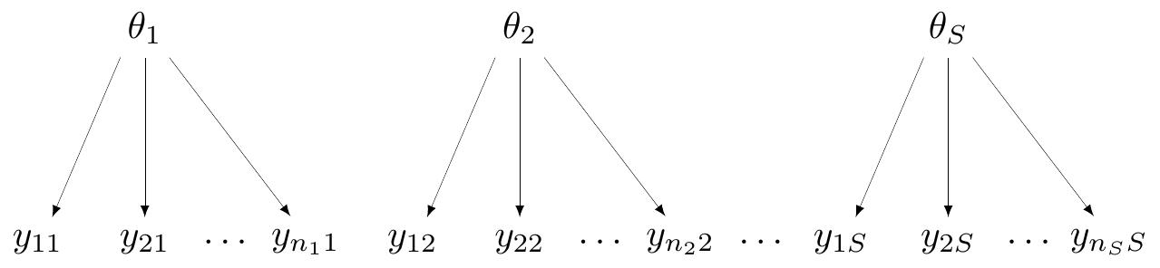
Here, the observed data are represented at the bottom of the graph and labelled as \(\boldsymbol{y}_s=(y_{1s},y_{2s},\ldots,y_{n_s s})\), for each of the \(s=1,\ldots,S\) groups (say, studies) considered. Generally speaking, while each study will be based on individual-level data such as \(\boldsymbol{y}_s\), in reality, when working with evidence synthesis we are more likely to actually access only a summary, for instance the total count for the occurrence of the event under study, \(r_s\), in the magnesium example.
In Figure 6.1, each study is assumed to follow a data-generating process that depends on a specific parameter (in this case, labelled as \(\theta_1,\theta_2,\ldots,\theta_S\)). Effectively, there is no connection whatsoever across the \(S\) studies and the data in each of them contribute solely to the estimate of the study-specific parameter, an assumption encoded by \(\theta_1,\ldots,\theta_S \stackrel{iid}{\sim} p(\cdot)\).
In the magnesium example, this assumption amounts to modelling \(\alpha_s\) and \(\delta_s\) independently \[ \alpha_s, \delta_s \stackrel{iid}{\sim}\text{Normal}(0,sd), \tag{6.5}\] for some suitable value of the standard deviation \(sd\).
Figure 6.2 is a specific version of the more general Figure 6.1, with reference to the magnesium example. Note that we explicitly include in the DAG representation the core parameters \((\alpha_s,\delta_s)\), of which the probabilities \(\pi_{st}\) are just transformations nodes that are defined as deterministic function – in fact, we could write the model in Equation 6.1 as \[r_{st} \sim \text{Binomial}(\underbrace{\text{logit}^{-1}\left(\alpha_s + \delta_s(\text{Trt}_{st}-1)\right)}_{\pi_{st}},n_{st}).\] However, for ease of representation, we omit from the DAG the constant \(\text{Trt}_{st}\).
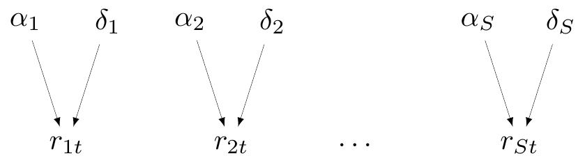
The model with “no-pooling” is not very helpful for the purpose of evidence synthesis, but it may be the most appropriate, for instance if we have some knowledge to deem (some of) the studies fundamentally different.
6.2.2 Complete pooling
At the other extreme, we may be willing to assume that all the studies are generated by the exact same mechanism and thus they share a common effect. A generalised version of this assumption can be shown graphically in Figure 6.3. Here, all the data points across the \(S\) studies depend on a single, common parameter \(\theta\) – this model is often referred to as “fixed effects”, particularly in a non-Bayesian context.
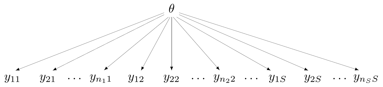
In this case, all the data are connected (and thus, in principle, strongly dependent) through the single DGP that we are assuming. This is of course the most useful assumption in terms of pooling and producing a precise estimate of the parameter \(\theta\). However, of course, complete pooling does represent a very strong modelling formulation, which is often difficult to defend dogmatically, as studies may embed inevitable heterogeneity (by design, measurements, inclusion/exclusion criteria, etc.).
In the case of the magnesium example, the complete pooling model is characterised by the assumption that \[ \delta_s = d \quad \mbox{for all } s=1,\ldots,S. \tag{6.6}\]
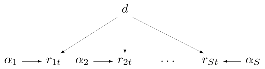
Figure 6.4 shows the DAG for this modelling assumption. Here, technically, the \(\alpha_s\) parameters are in fact specified for each different study; however, they essentially represent some “background noise” (i.e. the baseline for the probability of death) and the key parameter is the treatment effect \(d\), which is assumed to be just one and common across all studies.
6.2.3 Partial pooling (hierarchical models)
An intermediate situation is represented by the assumption of partial pooling, sometimes referred to as “random effects”. In a more general case, partial pooling can be depicted as in Figure 6.5, which can be seen as a compromise between the representations of Figures 6.1 and 6.3.
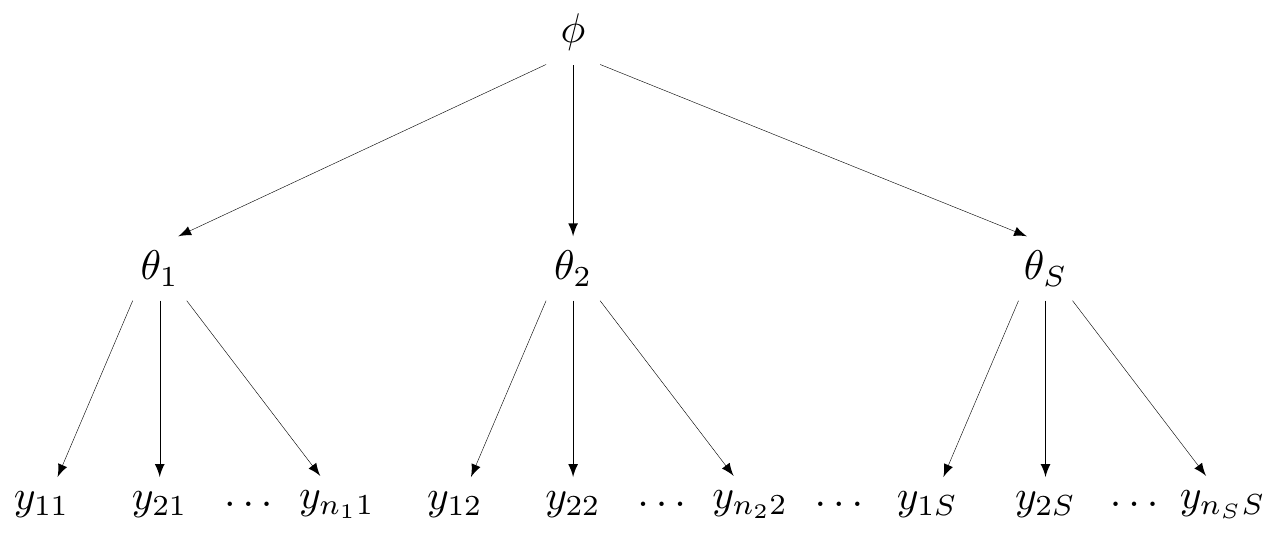
In each of the \(S\) studies, the data \(\boldsymbol{y}_1,\boldsymbol{y}_2,\ldots,\boldsymbol{y}_S\) are assumed to be generated by study-specific parameters \(\theta_1,\theta_2,\ldots,\theta_S\), exactly as in Figure 6.1. However, in the spirit of Figure 6.3, the study-specific parameters are also assumed to be subject to a common data-generating process, which is governed by a “hyper-parameter”, indicated as \(\phi\) in Figure 6.5.
Generally speaking, this implies a factorisation of the overall prior distribution as \[ p(\theta_1,\ldots,\theta_S,\phi) = p(\phi)\prod_{s=1}^{S} p(\theta_s\mid\phi). \]
NoteFixed vs random effects
In a Bayesian context, the distinction between fixed and random effects is not very helpful – in fact, perhaps even a bit confusing. In both cases, within a Bayesian framework, the relevant parameters are random, in the sense that we associate a probability distribution with them, to describe our uncertainty before seeing the data.
The real difference between the two models is in fact in the assumption we make for the distribution – following the phrasing suggested by Gelman and Hill (2007), in the former case, we use an “unstructured” approach, where the study-specific effect is assumed to be “fixed” across all the studies (i.e. there is a single \(d\) parameter, in the magnesium case); in the latter, we use a rather “structured” approach, where the various study-specific parameters are modelled using a common data-generating process.
For this reason, a better terminology (especially from a Bayesian perspective) would be to identify the two model specifications as “structured” vs “unstructured” effects (as opposed to “random” vs “fixed” effects).
This slightly more complex model formulation is often referred to as “hierarchical” or “multilevel”, to highlight the fact that we have several layers in our model. The evidence from the data will directly inform the study-specific parameters; however, because of the common “ancestor” \(\phi\), learning something about one of the study-specific parameter will allow us to also learn some information about all the others.
This process is sometimes referred to as “borrowing information” and it is particularly relevant if, for instance, one of the studies is small. In that case, the estimate for the corresponding parameter \(\theta_s\) is likely to be very imprecise, because of the lack of information in the data. However, through the implied correlation with all the other elements of the study-specific vector \(\boldsymbol\theta\), we can get a more precise estimate, by “borrowing” the information provided by the other studies. We return to this point in Section 6.2.7.
Under this setting, for the magnesium example, we would model \[ \begin{aligned} \delta_s & \sim \text{Normal}(d,\sigma_\delta) \\ d & \sim \text{Normal}(0,sd) \\ \sigma_\delta & \sim p(\sigma_\delta), \end{aligned} \tag{6.7}\] for a fixed value \(sd\) and a suitable prior distribution \(p(\sigma_\delta)\).
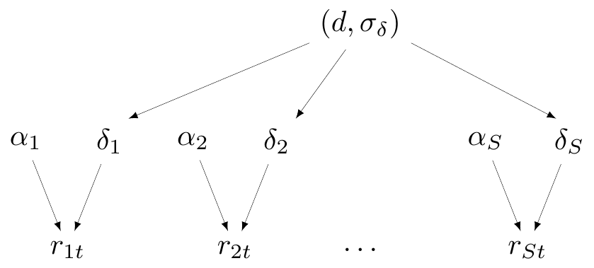
Figure 6.6 shows the DAG for partial pooling with specific reference to the magnesium example. To keep the parallel with Figure 6.5, here \(\boldsymbol\theta=(\boldsymbol\alpha,\boldsymbol\delta)\) and \(\boldsymbol\phi=(d,\sigma_\delta)\) are the hyper-parameters.
6.2.4 Exchangeability
An important implication of considering a hierarchical structure is the assumption of exchangeability across the study-specific parameters. From the technical point of view, exchangeability is a rather complex concept, first introduced by the work of Bruno de Finetti in the 1930s, although the definitive references for this are perhaps the later textbooks by de Finetti (1974) and Bernardo and Smith (1999).
Formally, a sequence of random variables \((y_1,\ldots,y_n)\) is judged to be exchangeable if our degree of belief in the occurrence of that sequence does not depend on the order in which the variables are observed. For example, considering \(n=3\) binary variables taking values \((0,1)\), exchangeability implies that \[\Pr(Y_1=1,Y_2=0,Y_3=1) = \Pr(Y_1=0,Y_2=1,Y_3=1) = \Pr(Y_1=1,Y_2=1,Y_3=0).\]
More pragmatically, a judgement of exchangeability implies that the variables under consideration are assumed to be similar, or to put it in a more technical way, that they are generated by a common process, which is governed by common random parameters.
Example 6.2. Pasta consumption and exchangeability (based on Gelman et al., 2013). Data are available from the 2012 International Pasta Organisation Annual Survey (yes: that is a real thing!) on the annual average per-capita pasta consumption (in kg).
You are told that 9 European countries have been selected and the average consumption of pasta has been recorded; these values are indicated as \(y_1,\ldots,y_9\). Notice that, at this stage, you do not know which countries have been selected for this study.
The concept of exchangeability can be explained making reference to “ignorance”. In the data, as currently provided, there is nothing for you to distinguish what the country associated with \(y_1\) may be, as opposed to that associated with \(y_9\), say.
We probably know something about the underlying target population, for instance that, generally speaking, European countries like pasta and make large use of it in their diets. But, for now, there is nothing in the data for us to be able to “tell which one is which”. Consequently, for the moment at least, it is probably reasonable to assume exchangeability, under this set up.
Imagine now that, out of the original 9 countries, we randomly select 8 and the actual observed results are the following (in kg): \[{4.4, 8.1, 6.6, 7.3, 8.1, 9.3, 7.5, 4.1.}\] Should this modify our assessment of exchangeability (or lack thereof)? And what should our best estimate of the value for the ninth European country, that has not been selected at this stage be?
The actual data (which now we get to see, at least partially) show some variability. There is a range of values, with some higher than others, but we may still assume that this is down to sampling variability and that all the observed values are drawn from a common data-generating process. In the absence of any other information, we may take the mean of the observed values (6.92kg per capita) as the “best estimate” for the missing country.
Now, suppose we are told that the 9 countries are: France, Latvia, Hungary, Portugal, Switzerland, Italy, Lithuania, Croatia, Germany – note that the order in which this information is presented is not the same in which the data are given. At this stage, we still do not know for which country the data have not been presented. Should this change your assessment of exchangeability (or lack thereof)?
Now we know that Italy is part of the sample and we may know how crazy Italians are about pasta. Thus, perhaps this may change your judgement – we may now think that the largest observed value is actually Italy, which means we would be able to distinguish one of the \(y\)-s from the others.
Or, perhaps, we may now be willing to stipulate that the missing value is Italy, which again would mean we would be able to tell some values apart from the others. Perhaps, at this stage, conditionally on all the information you now have, exchangeability would be broken and you may not be willing to assume it anymore.
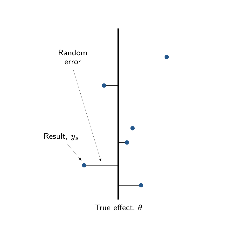
The main distinction between complete and partial pooling can be visualised in Figure 6.7. Figure 6.7 (a) shows that, under complete pooling, we are assuming a single, “fixed” true overall effect, \(\theta\); each study produces some observed results \(y_s\), which are subject to some random error, representing a deviation from the true overall mean, \(\theta\).
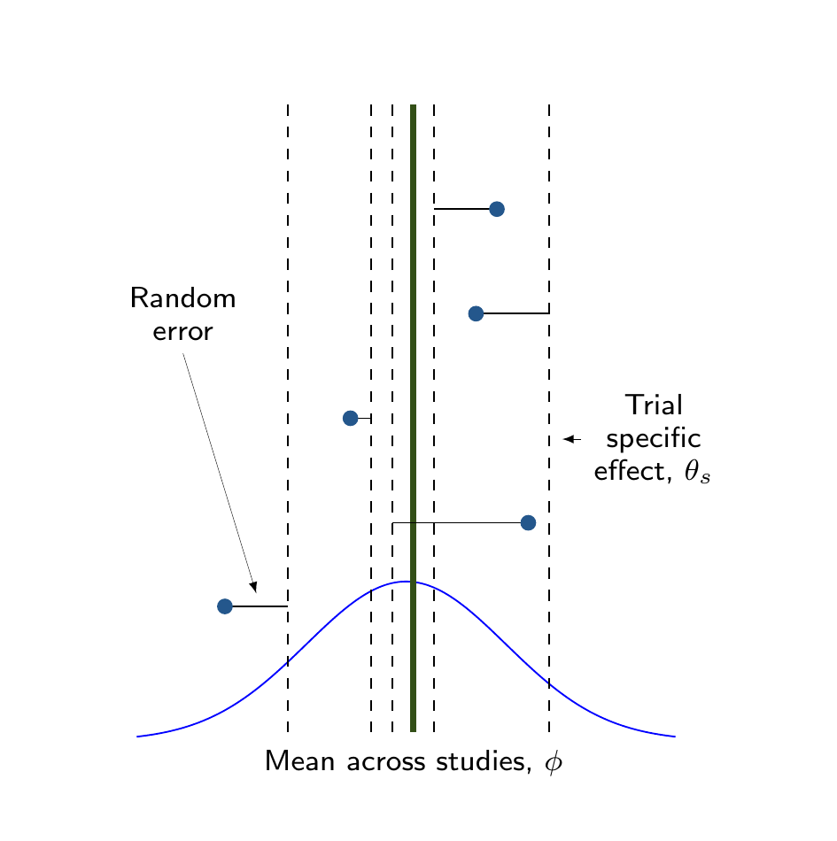
In Figure 6.7 (b), conversely, each study is characterised by a trial-specific effect \(\theta_s\) (the dashed vertical lines) and the study specific results (again described by the solid dots) are also subject to random errors with respect to that trial-specific effect. These, in turn, are drawn from a common distribution, whose mean \(\phi\) represents the overall pooled estimate.
Example 6.3. Magnesium (continued): no-pooling analysis. Assuming no other covariate is available or relevant, we could assume some very vague priors (i.e. \(sd \rightarrow \infty\)) on the regression coefficients \(\alpha_s\) and \(\delta_s\), defined in Equation 6.5. In the presence of large data, this would be, most likely, immaterial.
However, it would also be overly cautious and rather unnecessary – we are modelling the probability of death in the two arms on the logit scale. At face value, priors such as \(\alpha_s \sim \text{Normal}(0,sd=4)\) may look too restrictive and potentially bringing too much information in the analysis. Looking more closely, however, this actually implies a large variability, given the scale in which they are defined. We can check this using forward sampling (see Section 1.2.6), with the following code.
# Simulates 10000 values from the prior alpha_i ~ Normal(0,sd=4)
tibble(alpha=rnorm(10000,0,4)) |>
  # Rescales to probabilities applying inverse logit
  mutate(pi=exp(alpha)/(1+exp(alpha))) |> select(pi) |>
  # Uses 'bmhe' to summarise the simulations
  bmhe::stats()
mean sd 2.5% median 97.5%
pi 0.4975282 0.3974699 0.0003924477 0.4956394 0.9996017As is possible to see, the distribution for the resulting parameter pi, the probability that a random individual in the placebo arm dies, effectively spans the whole \([0;1]\) range.
Similarly, the parameters \(\delta_s\) represent the log OR for magnesium treatment, i.e. indicate how much more or less likely a random individual is to die if they are treated with magnesium, instead of placebo. We could go overboard and assume a very vague distribution, say \(\delta_s\sim\text{Normal}(0,sd=1000)\), so as to remove any bias in favour of the active treatment and “let the data speak for themselves”.
However, this is also a rather silly assumption, because we would be implying a ridiculous prior on the resulting OR, with extremely high and implausible values being given a large amount of probability, in the prior. Already assuming \(sd=2\) would imply a large range, when suitably rescaled.
# Simulates 10000 values from the prior alpha_i ~ Normal(0,sd=4),
# and delta_i ~ Normal(0,sd=2)
tibble(alpha=rnorm(10000,0,4),delta=rnorm(10000,0,2)) |>
  # Rescales to probabilities applying inverse logit
  mutate(pi=exp(alpha+delta)/(1+exp(alpha+delta))) |> select(pi) |>
  # Uses 'bmhe' to summarise the simulations
  bmhe::stats()
mean sd 2.5% median 97.5%
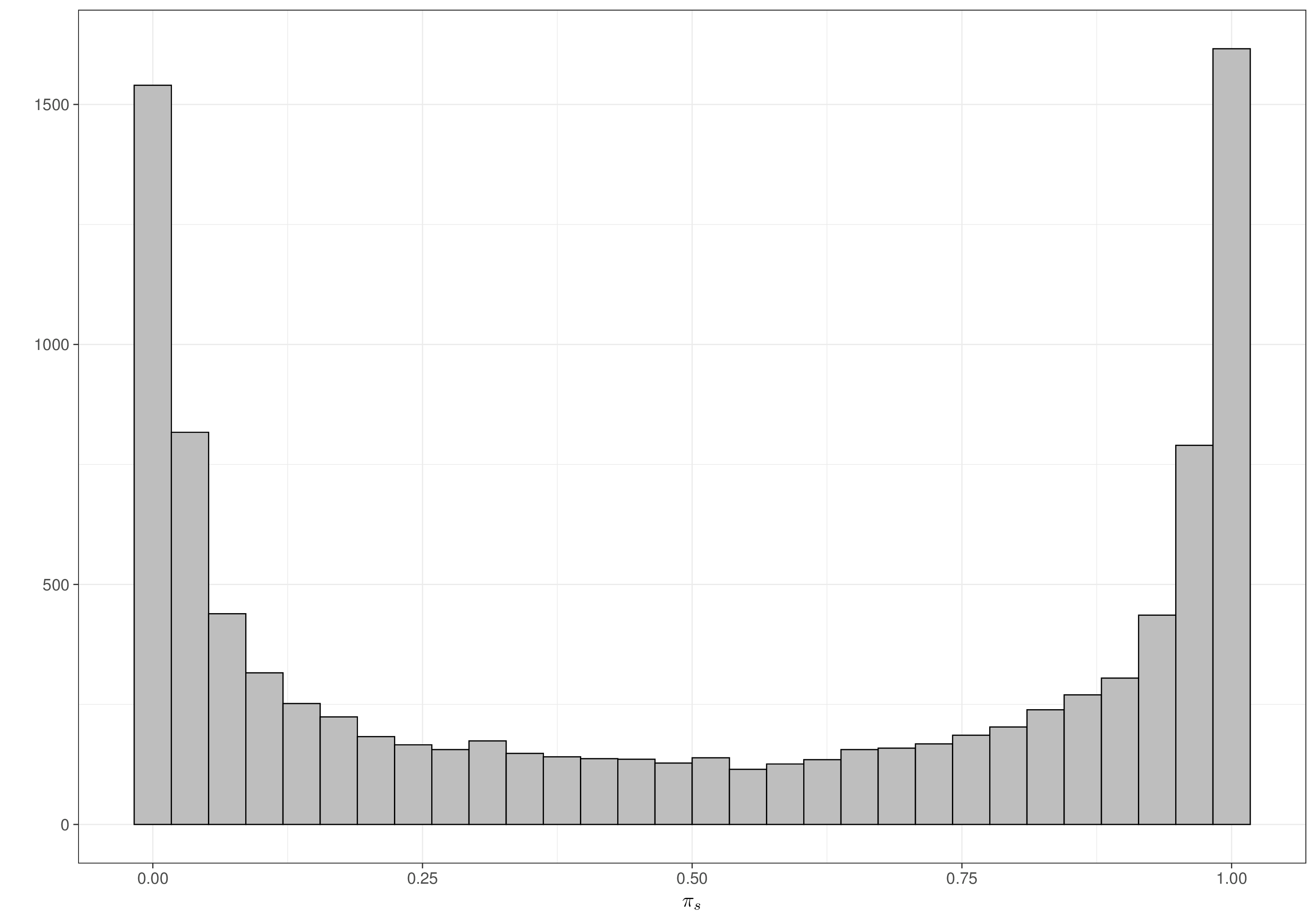
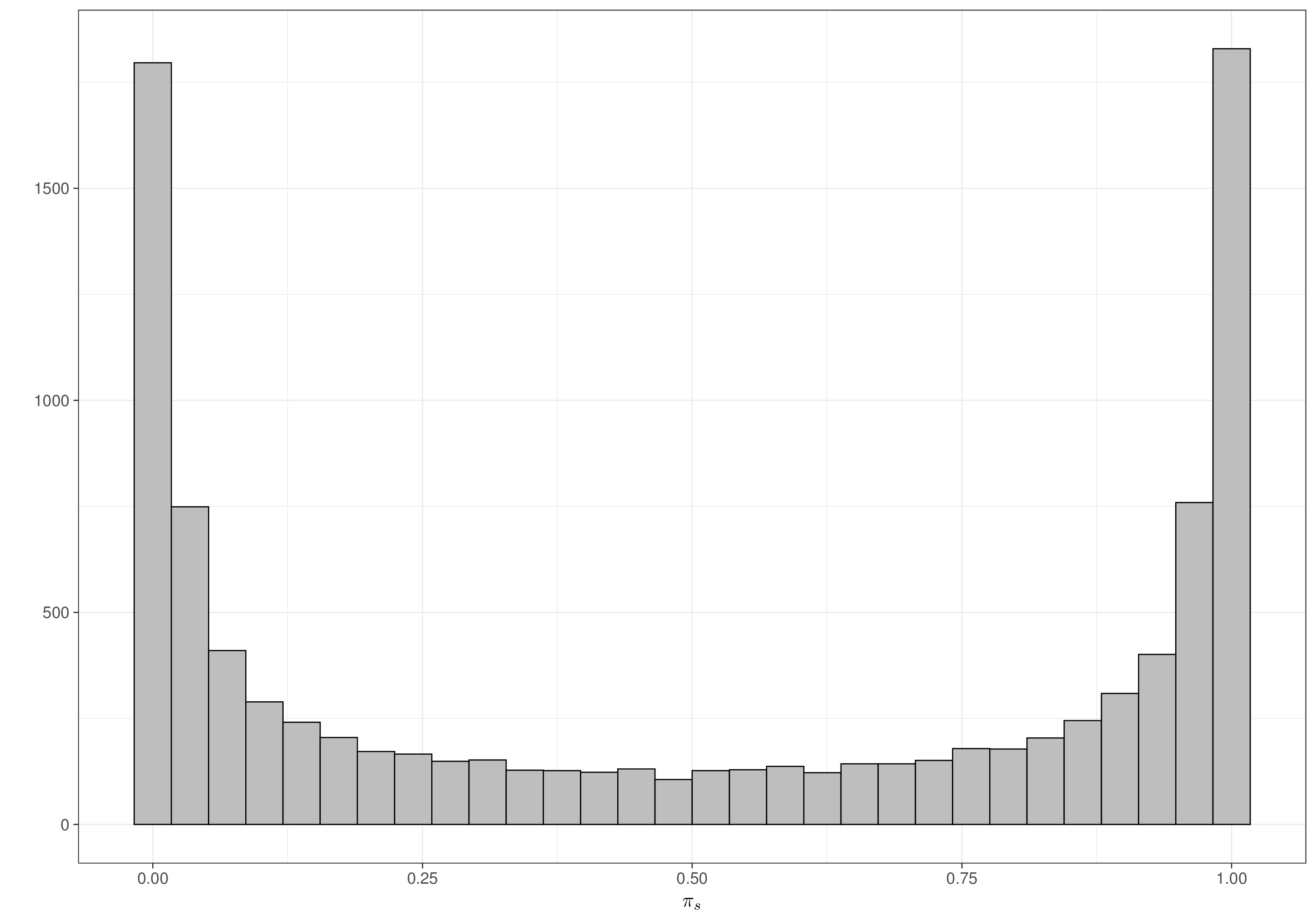
pi 0.5063376 0.4098462 0.0001353949 0.5208656 0.9998531Once again, when rescaled to the probability range, the distribution for pi, which in this case represents the probability of death for a random individual treated with magnesium, does effectively cover the whole \([0;1]\) range, indicating that even a seemingly informative prior, in this particular case, is vague enough. Figures 6.8 (a) and 6.8 (b) show the resulting prior for each of the \(\pi_s\), in the placebo and treatment arm, respectively – as is possible to see these distribution resemble closely the Jeffreys’ prior discussed in Note 2.1 in Example 2.5 and shown in Figure 2.10.
Crucially, we allow for sufficient mass at either end of the range (i.e. towards 0 or 1), which should be able to safeguard against marked heterogeneity in the individual studies estimates.
Note 6.2: The parachute effect
While we do not want to impose too strong priors on the “treatment effect”, there is much information that we can use to restrict the reasonable range of a log OR.
For instance, consider an experiment in which we test the effectiveness of parachutes, when jumping off a flying plane. We define our outcome \(Y\) as 0 if the individual jumps off the plane and dies and 1 if they survive. The treatment is measured through \(X_i\), taking value 1 if individual \(i\) is given a parachute and 0 otherwise.
In a situation such as this, we may expect the treatment to have a very large effect – almost everyone with a parachute can be reasonably expected to survive, while almost (or probably just!) everyone without one is most likely to die. So if we define \(\theta_1=\Pr(Y=1 \mid X=1)\) and \(\theta_0=\Pr(Y=1 \mid X=0)\), we could reasonably estimate something like \(\theta_1 =0.9\) and \(\theta_0=0.1\) (the actual numbers are irrelevant – but the magnitude is important and arguably realistic). Thus, in this case the OR would be \[ \begin{aligned}[t] \text{OR} & = \left. \frac{\theta_1}{1-\theta_1}\middle / \frac{\theta_0}{1-\theta_0} \right. \\ & = \left. \frac{0.9}{1-0.9} \middle / \frac{0.1}{1-0.1} \right.\\ & = \left. \frac{0.9}{0.1}\middle / \frac{0.1}{0.9} \right. = \left. 9 \middle / \frac{1}{9} \right. = 81. \end{aligned} \tag{6.8}\] This means that people with a parachute are 81 times more likely to survive the jump off the plane than those without a parachute. This massive OR comes about, of course, because of the assumptions we are making about such a large treatment effect – almost everyone without the parachute dies, while almost everyone with survives. In a case such as this, we may be prepared to believe a very large OR. But in most cases, interventions do not have such dramatic effects. And thus, it is reasonable to imagine that ORs greater than 3 or perhaps 4 are already relatively unlikely to be observed in practice!
We can write down the JAGS code for the no-pooling assumption as below.
no_pooling=function(){
  for(s in 1:S) {
  # Sampling distributions
    r1[s] ~ dbin(pi1[s], n1[s])
    r2[s] ~ dbin(pi2[s], n2[s])
    logit(pi1[s]) <- alpha[s]
    logit(pi2[s]) <- alpha[s] + delta[s]
  # Baselines (NB: sd=4 => precision = 0.0625)
    alpha[s] ~ dnorm(0,0.0625)
  # Study-specific treatment effects (sd=2 => precision = 0.25)
    delta[s] ~ dnorm(0,0.25)
  }
}
We can then run the model using R2jags – notice that we specify a function inits() which randomly generates initial values for alpha and delta. In this case, we choose a vector of 16 random draws from a \(\text{Normal}(0,1)\). This is not essential (and we could leave the generation of the initial values to JAGS, as we have done in all the examples in Section 5.2), but it is helpful to have the option, particularly for model that are a bit more complex.
Moreover, we use a relatively large number of simulations (10 000) and apply thinning of 1 every 4 simulations (so as to save 4000 iteration at the end of the process) – we do this to combat potential issues with autocorrelation, which we can expect, since we are assuming that each study is modelled independently with no possibility of “borrowing information” from the others. Thus, small studies or those where information is very sparse (e.g. study number 8, where there have been only 1 death in total, with very small sample sizes) will be harder to estimate, given the lack of definitive evidence in the data.
# Defines the data list
data=list(r1=r1,r2=r2,n1=n1,n2=n2,S=nrow(trials))

# Initialises the object 'model' as a list to store all the results
model=list()

# Stores the JAGS output
model$no_pooling=jags(
  data=data,
  parameters.to.save=c(
    "alpha","delta"
  ),
  inits=function(){
    list(alpha=rnorm(16,0,.5),delta=rnorm(16,0,.5))
  },n.chains=2,n.iter=10000,n.burnin=2000,n.thin=4,DIC=TRUE,
  model.file=no_pooling
)
We can visualise the diagnostic measures for the model, using the bmhe::diagplot() function (and customising it using ggplot2 facilities), as shown in Figure 6.9.
# Rhat
bmhe::diagplot(model$no_pooling)

# n.eff
# Highlights all parameters where n.eff < 10% of the nominal sample size (400)
bmhe::diagplot(model$no_pooling,what = "n.eff",label=TRUE) +
  geom_hline(yintercept=400, linetype="dashed") +
  annotate("rect",xmin=-Inf,xmax=Inf,ymin=-Inf,ymax=400,alpha=0.2,fill="gray70")

# Traceplots for selected nodes (below 10% of the nominal number of simulations)
bmhe::traceplot(
  model$no_pooling,parameter=which(
    model$no_pooling$BUGSoutput$summary[,"n.eff"]<400
  ) |> names()
)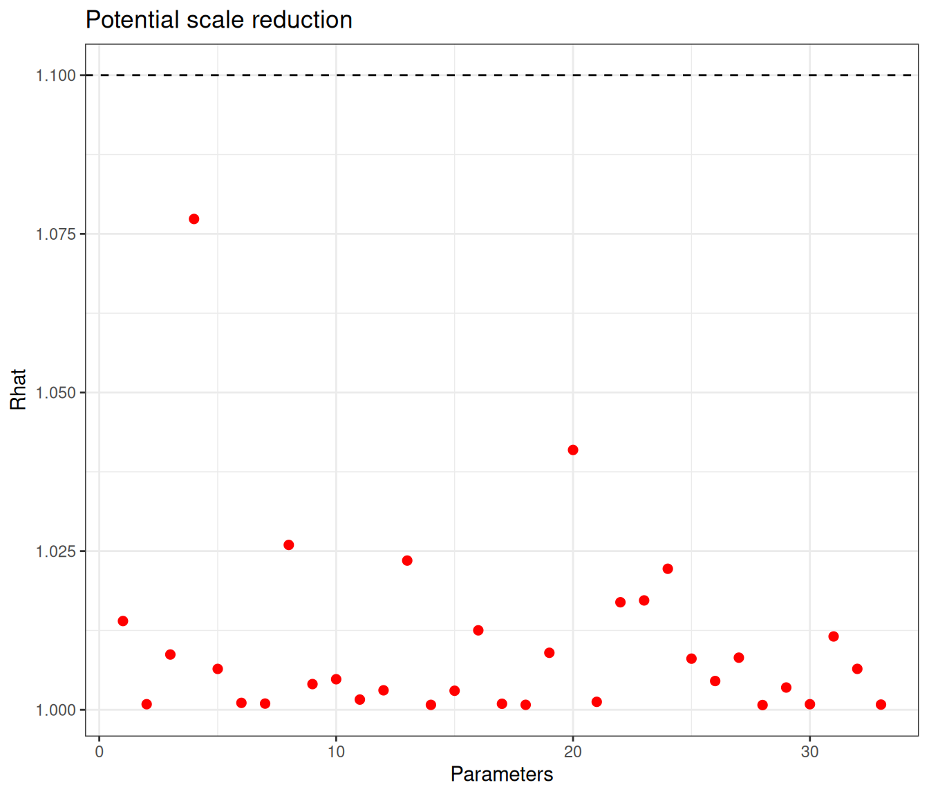
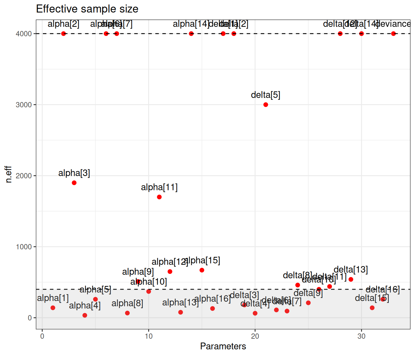
Figure 6.9 (a) generally indicates satisfactory convergence for the model – looking at the \(\hat{R}\) statistic, almost all nodes have values below the cutoff of 1.1. Even with thinning and a long run, autocorrelation seems to impact quite a few parameters, for which the effective sample size is rather low. Figure 6.9 (b) shows the value of the effective sample size for each of the model parameters – we have highlighted in the grey area the few ones with ESS below 10% of the nominal sample size (i.e. 400).
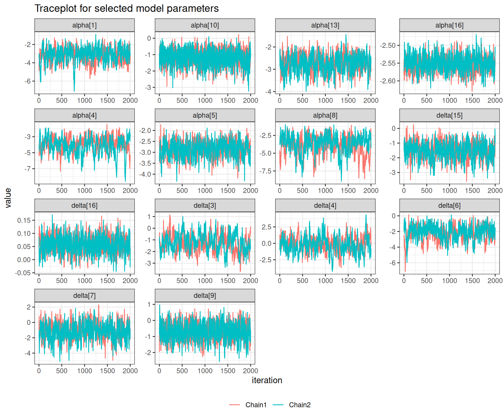
There are not very many of them and thus, on this occasion, we may still be satisfied with the convergence of the model, although perhaps we may want to run for an even longer number of iterations or test different specifications for the priors. This is confirmed by the analysis of the traceplots for these nodes, which is depicted in Figure 6.10, in which all seem reasonably mixing, despite the larger autocorrelation.
NoteThe art of setting priors
Notice that there is nothing special whatsoever to the values of 4 and 2 for the standard deviations of \(\alpha_s\) and \(\delta_s\) – these choices should be dictated by contextual knowledge, as well as subject to substantial sensitivity analysis.
For example, we could use a “lazy” option and set priors for \(\alpha_s,\delta_s\stackrel{iid}{\sim}\text{Normal}(0,sd=100)\). In this case, for most parameters, the choice of priors would not make a difference – not to in a tangible fashion, anyway. However, it is likely that the node delta[8] would struggle to converge, if we used a very wide, “non-informative” prior.
This is not entirely surprising: study number 8 (Bertschat) in Table 6.1 has very low numbers of observed deaths (only 1 in the placebo arm and none in the magnesium arm, in correspondence of very small sample sizes too). For this reason, the estimate for the log OR parameter \(\delta_8\) can be highly unstable, particularly if we do not “help” by suggesting a reasonable range in the prior, given that we take every study as separate in the no-pooling model.
Example 6.4. Magnesium (continued): complete-pooling analysis. We can code up the model in Equations 6.1 and 6.6 into the following JAGS code. Notice that we use here the following prior specification: \(\alpha_s \sim \text{Normal}(0,sd=4)\) and \(d\sim\text{Normal}(0,sd=2)\), in line with the model used in Example 6.3.
complete_pooling=function() {
  for(s in 1:S) {
  # Sampling distributions
    r1[s] ~ dbin(pi1[s], n1[s])
    r2[s] ~ dbin(pi2[s], n2[s])
  # Model
    logit(pi1[s]) <- alpha[s]
    logit(pi2[s]) <- alpha[s] + d
  # Baselines
    alpha[s] ~ dnorm(0,0.0625)
  }
  # Priors
  d ~ dnorm(0,0.25)
  OR <- exp(d)
}
In addition, now that we have a (rather strong) form of pooling across the various studies, we are able to produce an overall measure of treatment effect. We can simply rescale the parameter \(d\) by exponentiating it to obtain an overall OR – the node OR indicates the odds ratio for magnesium treatment, or, in other words, a measure of how more likely a random individual is to die if they are treated with magnesium, rather than with placebo.
The model is run using code all but identical to that shown in Example 6.3 – we just change the name of the output to the object model$complete_pooling and point the execution of JAGS to the function describing the relevant model, model.file=complete_pooling in this case. We use again a relatively long run with 40 000 iterations and thinning of 18, to limit the impact of autocorrelation.
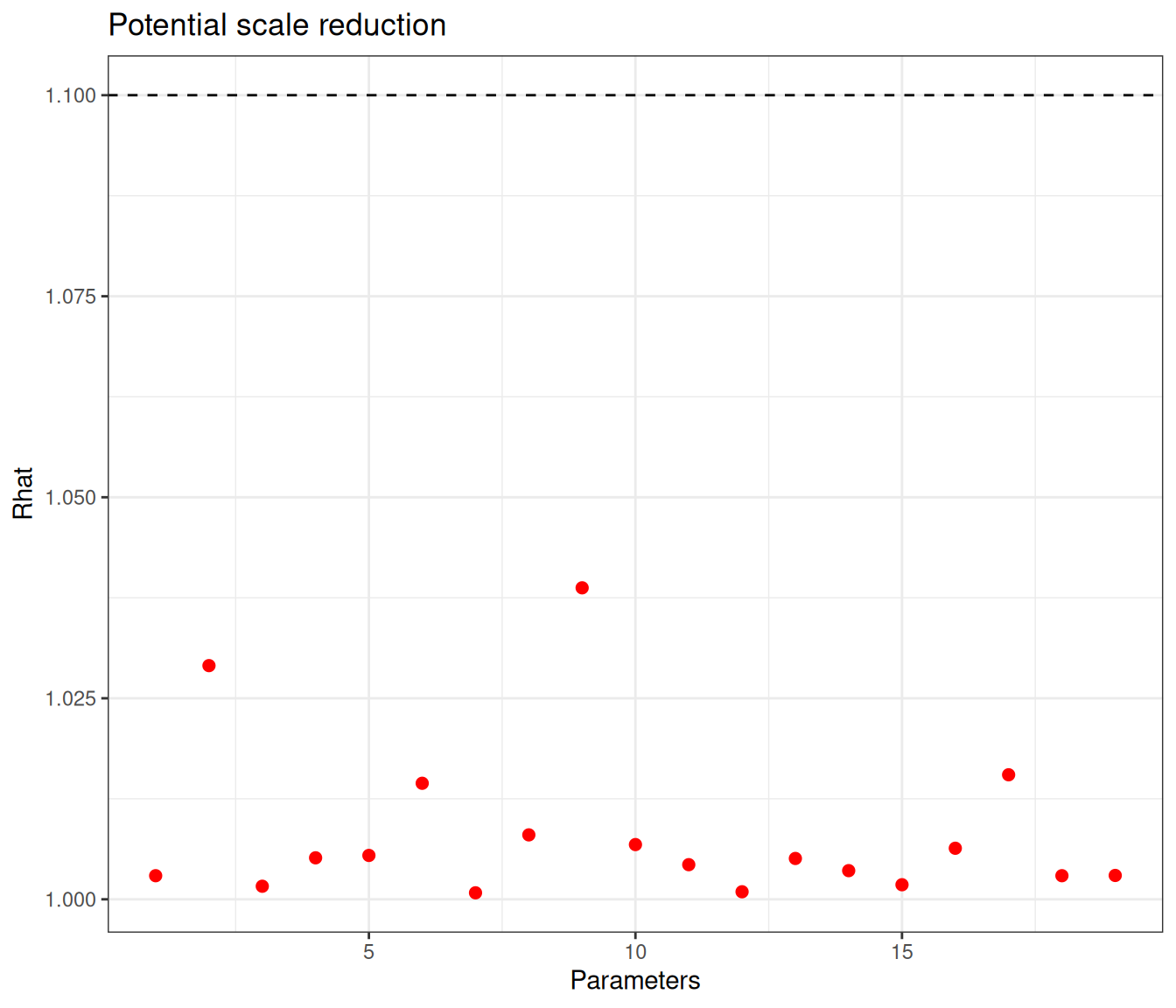
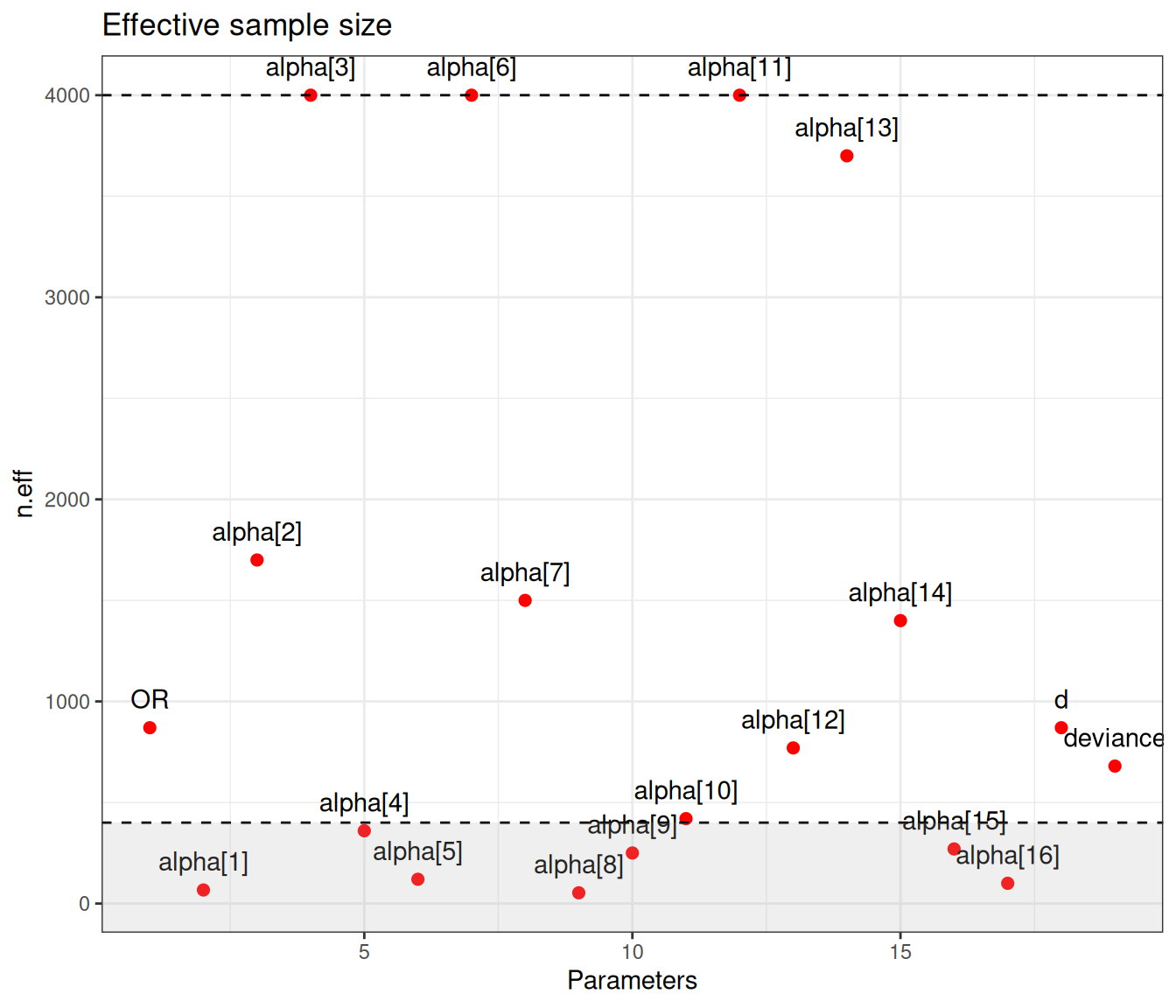
Figure 6.11 shows graphical summaries for the model diagnostics – again, with the selected model specification, convergence is reached (according to the threshold of 1.1 for the \(\hat{R}\) statistic) for all nodes. There are a few that are still subject to some substantial autocorrelation – this time only 7 (alpha[1], alpha[4], alpha[5], alpha[8], alpha[9], alpha[15] and alpha[16]) are below the cutoff of 10% of the nominal sample size, again set at 4000 iterations, but, all in all, we may be satisfied with the model convergence.
Example 6.5. Magnesium (continued): partial-pooling analysis. We complete the range of models for the magnesium trials fitting the hierarchical version of Equation 6.7. In this case, we still keep the prior for \(\alpha_s \sim \text{Normal}(0,sd=4)\), implying a precision of 0.0625. As for the structured effects \(\delta_s\), we model their standard deviation using a PC prior, encoding the assumption that \(\Pr(\sigma_\delta>1) \approx 0.1\), giving an \(\text{Exponential}(2.31)\) – see Example 2.5. Finally, the pooled estimate \(d\), which represents the mean around which all the \(\delta_s\) are distributed, is given a minimally informative prior \(\text{Normal}(0,sd=2)\).
Notice also that, this time, we are able to produce two different pooled summaries. The first one is the same as in Example 6.4, i.e. the pooled \(\text{OR}=\exp(d)\). The second is based on the predictive distribution of the treatment effects \(\delta_s\) – this can be interpreted as the prediction for an entirely new study, assumed exchangeable with the 16 analysed thus far. Exponentiating the node delta.pred would provide an estimate of the OR for this new study.
The model is defined in the following R code
partial_pooling=function(){
    for(s in 1:S) {
  # Sampling distributions
    r1[s] ~ dbin(pi1[s], n1[s])
    r2[s] ~ dbin(pi2[s], n2[s])
  # Model
    logit(pi1[s]) <- alpha[s]
    logit(pi2[s]) <- alpha[s] + delta[s]
  # Baselines
    alpha[s] ~ dnorm(0,0.0625)
  # Random Effects
    delta[s] ~ dnorm(d, prec)
  }
  # Priors
  d ~ dnorm(0,0.25)
  # Pr(sigma.delta>1) \approx 0.1
  sigma.delta ~ dexp(2.31)
  prec <- pow(sigma.delta,-2)
  # Summaries
  OR <- exp(d)
  delta.pred ~ dnorm(d, prec)
}
and can be run using code similar to the one used for the previous models. We store the output in an object model$partial_pooling and set model.file=partial_pooling.
Similarly to the previous analyses, we can check the diagnostics using Figure 6.12.
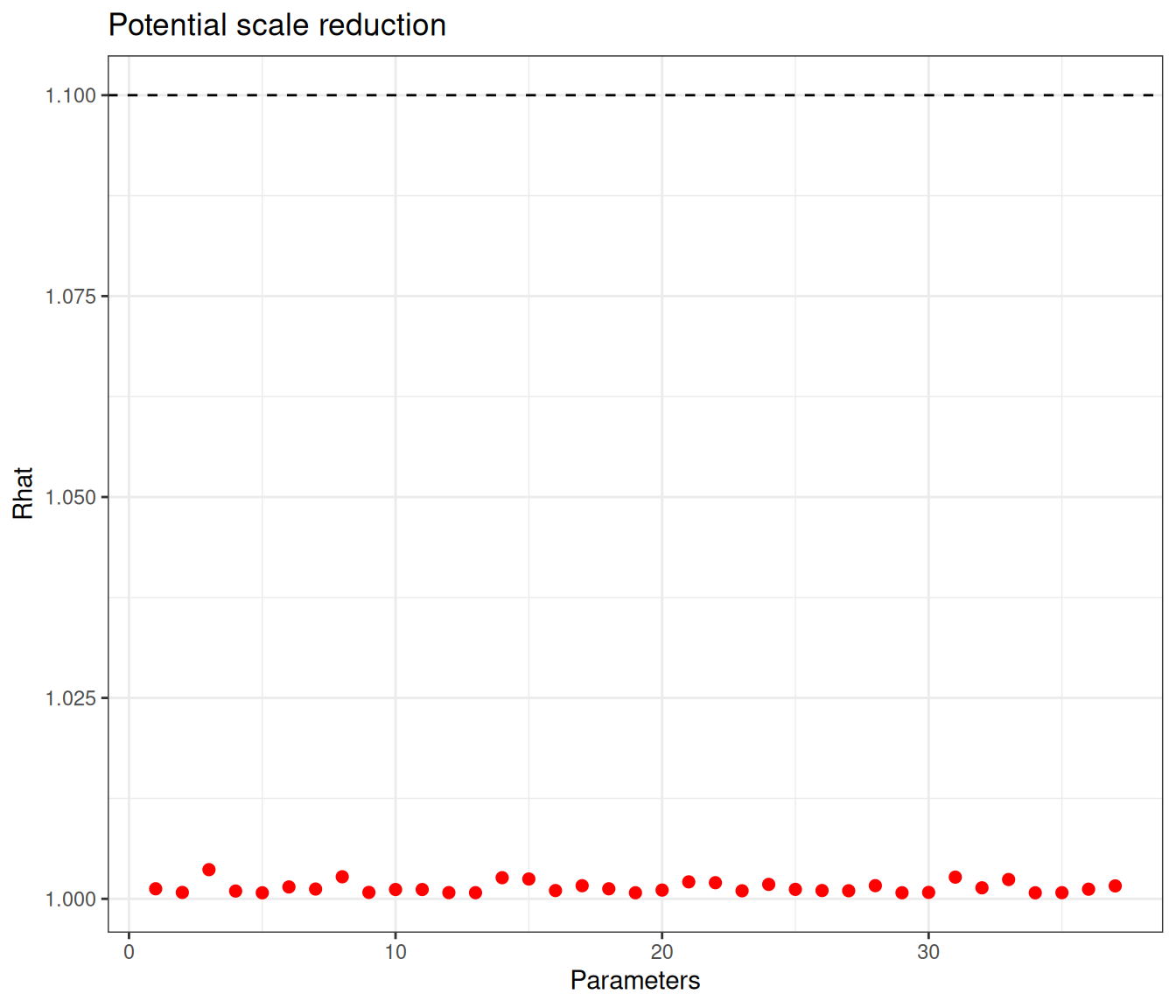
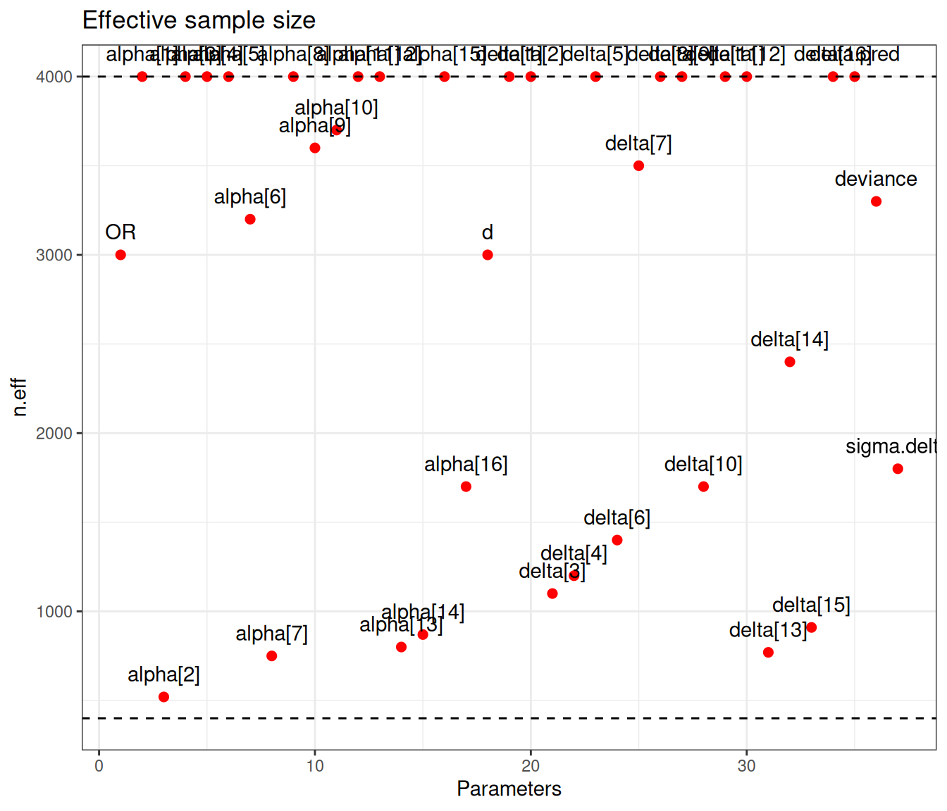
This time convergence is really not an issue – all nodes show values for \(\hat{R}\) well below 1.1 and none of the nodes has an effective sample size that is below 10% of the nominal one. The information is shared across all the studies, through the hierarchical structure.
The model code and discussion above highlights how the partial pooling is effectively a bigger version of the model for evidence synthesis, which includes as special cases the two extremes of no- and complete pooling. In fact, from the model in Equation 6.7 we can derive the complete pooling by setting \[ \delta_s \sim \text{Normal}(d,\sigma_\delta=0) \] — if the standard deviation in the distribution of the structured effects is 0, then there is no variability across them and so each one of them is identical with their mean, \(d\), exactly as in Equation 6.6.
Similarly, if we set \[ \delta_s \sim \text{Normal}(d,\sigma_\delta\rightarrow \infty) \] then the variations across the structured effects are so large that each \(\delta_s\) is different from the others and, crucially, they become unrelated – just like in Equation 6.5.
6.2.5 When should we use hierarchical models?
Intuitively, the discussion above suggests that we probably are better off at least testing a hierarchical version of the model: if the data provide no evidence for pooling, then the model will respond by estimating \(\sigma_\delta \rightarrow \infty\); if on the other hand, the data indicate little or no heterogeneity, then, in the posterior, \(\sigma_\delta \rightarrow 0\). The strong assumptions encoded in either of the two extreme versions of the model are much less flexible.
Of course, if we only have a small number of groups (e.g. studies) to pool across, then using hierarchical models becomes a bit more complicated, because we would have very little information to estimate the standard deviation \(\sigma_\delta\). Gelman and Hill (2007) suggest that we need at least 3 groups for a “vanilla” hierarchical model to work – this is of course sensible, because with only 2 data points, any estimate for a standard deviation is highly unstable.
From a purely Bayesian perspective, however, even low number of groups does not pose an impossibility to the use of partial pooling – this simply means that the information present in the data is sparse and, as such, in order to have consistent inference, we need to complement it with strong prior assumptions. More importantly, generally speaking, we need to be careful when setting models for the standard deviation of the “random effects” – unless we have a large amount of data over a large number of groups, we probably will not be able to get away with lazy, vague priors.
For instance, a model with \(\sigma_\delta\sim\text{Uniform}(0,K)\) for some constant \(K\) is often suggested and used in applied work. Again, this may work well if there is enough information in the data and, more importantly, if this information is strong enough to “travel against the arrow” in Figure 6.5 – there is a long way from the evidence in the bottom layer of the DAG (the data \(y_{1s},y_{2s},\ldots,y_{{n_s} s}\)) to update first the “level 1” parameters (\(\theta_1,\ldots,\theta_S\)) and then the hyper-parameter \(\phi\).
A subtle artifact of using this modelling structure with insufficient data/groups is that, in the posterior, \(\sigma_\delta\) will tend to push to the upper range of the Uniform. Thus, in the absence of firm evidence, a model with this prior will probably have a posterior for the standard deviation of the hyper-parameter highly concentrated towards \(K\) – but note that, of course, no matter what the data say, a Uniform prior will not allow the posterior to have any mass outside of the range (\([0; K]\), in this case).
The PC prior that we have used in Example 6.5 is certainly a good compromise, because while not implying unduly strength in the prior, it manages to stabilise the inference and does allow for values that are larger than where most of the mass is, in the prior. We thus recommend the use of this formulation and discourage other options, such as the conjugate vague \(\text{Gamma}(\varepsilon,\varepsilon)\) on the precision scale, for a small constant \(\varepsilon\) (say 0.001), or the \(\text{Uniform}(0,K)\) for the standard deviation – see Note 6.3 below, for a more detailed discussion.
Another useful alternative is the Half Cauchy model with location \(\mu=0\) and scale \(\lambda\), suggested by (Gelman, 2006), which is often implemented as the default in Stan. This is equivalent to modelling \[
\sigma_\delta \sim \text{Cauchy}(\mu=0,\lambda)\mathbb{I}(0,\infty),
\] where, in general \[
y \sim \text{Cauchy}(\mu,\lambda) \quad \Rightarrow \quad p(y\mid \mu,\lambda) = \pi\lambda \left(1+\left(\frac{y-\mu}{\lambda}\right)^2\right)^{-1}
\tag{6.9}\] (with the Half Cauchy, we restrict the expression in Equation 6.9 to \(\mathbb{R}^+\), as we are modelling a standard deviation) – see Example 7.3 for more detailed discussion. Gelman and Hill (2007, p. 428) also provide more details on the definition and use of Half Cauchy distributions in hierarchical models.
Note 6.3: The problem with Gamma priors on the precision
A \(\text{Gamma}(\alpha,\beta)\) prior on the precision (defined as in Equation 1.2) implies \[ \sigma^2 \sim \text{Inverse-Gamma}(\alpha,\beta) \quad\Rightarrow\quad p(\sigma^2) = \frac{\beta^\alpha}{\Gamma(\alpha)}\sigma^{-2(\alpha+1)}\exp\left(-\frac{\beta}{\sigma^2}\right) \tag{6.10}\] – we can derive this applying the change of variable rule in Equation 1.14 with \(\sigma^2=1/\tau\). As \((\alpha,\beta)\rightarrow 0\), this becomes a proper version (i.e. it still integrates to 1 over the range of \(\sigma^2\)) of the Jeffreys’ prior \(p(\sigma^2)\propto \frac{1}{\sigma^2}\) (see the general discussion in Note 2.1 in Example 2.5).
Together with the fact that a Gamma is conjugated for a precision (see Equation 2.9 and Example 2.7), this has made Equation 6.10 a popular choice to give a conjugate, vague prior to model precisions/variances, often used uncritically in applied work, especially early on in the BUGS revolution of the 1990s.
In the context of hierarchical modelling, however, Gelman (2006) has shown that there are some potential pitfalls to this particular choice. Applying again Equation 1.14, we can derive the implied prior on the scale of the standard deviation, using the following relationships: \[ \sigma = \frac{1}{\sqrt{\tau}} \Rightarrow \tau = \frac{1}{\sigma^2} = \sigma^{-2}, \] which imply that \[\begin{eqnarray*} \left\lvert \frac{\partial \sigma^{-2}}{\partial \sigma} \right\rvert = \left\lvert -2 \sigma^{-3} \right\lvert = 2\sigma^{-3} \!\!\quad\!\! \Rightarrow \!\!\quad\!\! p(\sigma) & \!\!\!\! = & \!\!\!\! \frac{\beta^\alpha}{\Gamma(\alpha)}\sigma^{-2(\alpha-1)}\exp\left(-\frac{\beta}{\sigma^2}\right) 2\sigma^{-3} \\ & \!\!\!\! = & \!\!\!\! \frac{2\beta^\alpha}{\Gamma(\alpha)}\sigma^{-(2\alpha+1)}\exp\left(-\frac{\beta}{\sigma^2}\right) \\ & \!\!\!\! \propto & \!\!\!\! \sigma^{-(2\alpha+1)}\exp\left(-\frac{\beta}{\sigma^2}\right). \end{eqnarray*}\]
This formulation tends to have extremely heavy right tail, which in turn implies that very large values of \(\sigma\) are highly probable. When data are directly observed to estimate the variance parameter, this may not matter much. But in the case of hierarchical models, the parameter of interest (e.g. \(\sigma_\delta\)) is only informed indirectly by the data – see Figure 6.5, which may lead to unintended (and dangerous) consequences.
This is because the use of (an approximation to) the Jeffreys’ formulation for the precision means that, while we do not mean to imply a strong prior near 0 (and thus towards large values for the variance (see the discussion in Note 2.1 in Example 2.5), the Bayesian machinery takes this information at face value and the standard deviation may be unduly pulled towards large values, implying excess of heterogeneity – cfr. Section 6.2.5.
We can easily check using Monte Carlo forward sampling, as with the following code.
# Simulates from the prior for the precision
tau=rgamma(10000,shape=0.001,rate=0.001)
# Computes tail-area probabilities
sum(tau>0.001)/length(tau)
[1] 0.0141Under this formulation for the precision, there is very, very little chance of exceeding values as small as 0.001! Consequently, as the whole distribution for the precision is highly concentrated towards 0, the resulting distribution for \(\sigma\) will exhibit a large number of large values and thus a model based on this assumption will often infer a very large standard deviation, even when the data show little support to it.
Conversely, while still allowing to control for the amount of mass placed above a certain threshold, e.g. in our case \(\Pr(\sigma_\delta>1)\), using a Half-Cauchy or a PC prior tends to spread the mass over a large enough range of possible values, while leaving the posterior free to move towards specific values, given the support from the data. In addition to this, by being directly defined on the scale of interest, it is easier to include even minimal information and thus we prefer and recommend it, at least as a default choice.
6.2.6 Model selection
As we have seen in Section 5.3, one simple criterion to perform model selection, or at any rate, to assess the performance of competing models in terms of fitting to the same data, is to use the DIC. Because in all the examples above, we have used 2 chains to run the Gibbs sampling via JAGS, this is automatically computed and stored, together with the penalty.
We can extract the penalty and the DIC from an object x generated by a call to R2jags::jags() simply calling the elements x$BUGSoutput$pD and x$BUGSoutput$DIC. For the three models stored in the elements of the object model, created in Example 6.3 and then populated in Examples 6.4 and 6.5, the resulting values are presented in Table 6.2.
| Model | \(p_V\) | DIC | \(\text{E}\left[D(\boldsymbol\theta)\right]\) | \(\text{sd}\left[D(\boldsymbol\theta)\right]\) |
|---|---|---|---|---|
| No-pooling | 30.20 | 177.93 | 147.74 | 7.77 |
| Complete pooling | 16.14 | 211.14 | 195.00 | 5.69 |
| Partial pooling | 26.38 | 173.47 | 147.10 | 7.26 |
As is possible to see, the values are substantially different across the three models – the partial pooling model has values for the DIC smaller than for the other two models. This indeed indicates a better performance of the hierarchical model, particularly against the complete pooling model.
Ultimately, the analysis of Table 6.2 strongly suggests that the partial pooling model should be used here, to cope with the inherent heterogeneity across the studies. We can also compute the penalty as \(p_D\) (as in Equation 5.14), which provides a more direct assessment of the amount of correlation across the structured effects, which the model is able to detect.
6.2.7 Borrowing information
Intuitively, the no-pooling model of Example 6.3 has a nominal number of parameters equal to the sum of the number of \(\alpha_s\) parameters and the number of \(\delta_s\) parameters, resulting in \(16+16=32\). This is because they are the only parameters included in the model and there is no sharing of information/correlation implied.
At the other extreme, the complete pooling model of Example 6.4 has 16 \(\alpha_s\) parameters in addition to the pooled effect, \(d\) and thus, in total, 17 parameters, nominally.
For the partial pooling model of Example 6.5, things are a bit more complicated: there are 16 \(\alpha_s\), as well as, nominally, 16 \(\delta_s\) in addition to the pooled log OR, \(d\), the predicted log OR (\(d_{pred}\)) and the standard deviation of the structured effects \(\sigma_\delta\). At face value, we thus have 35 parameters. However, because we are implying correlation across the \(\delta_s\), through the hierarchical structure, the number of effective parameters (which is estimated by \(p_D\) – but, in general, not by \(p_V\); recall the discussion in Section 5.3) is generally reduced. The amount of “shrinkage”, i.e. how many effective parameters are saved by the hierarchical structure, is a measure of how much correlation the model is able to pick up.
Example 6.6. Magnesium (continued): analysis and model comparison. As discussed in Section 5.3, we can compute an approximation to the version of the penalty defined in Equation 5.14 using the function rjags::dic.samples(), which returns the estimated \(p_D\) (penalty) and the resulting DIC (Penalized deviance) – notice however, that we can compute both versions of the penalty by adding the input pD=TRUE to the call to the function R2jags::jags().
Figure 6.13 shows the overall value for the DIC for the three models, partitioned into the contribution of the average deviance, \(\overline{D(\boldsymbol\theta)}\) and the estimate of the effective number of parameters, \(p_D\). As it is often (but not necessarily always) the case, the estimates for \(p_V\) and \(p_D\) are fairly aligned with very minimal numerical differences.
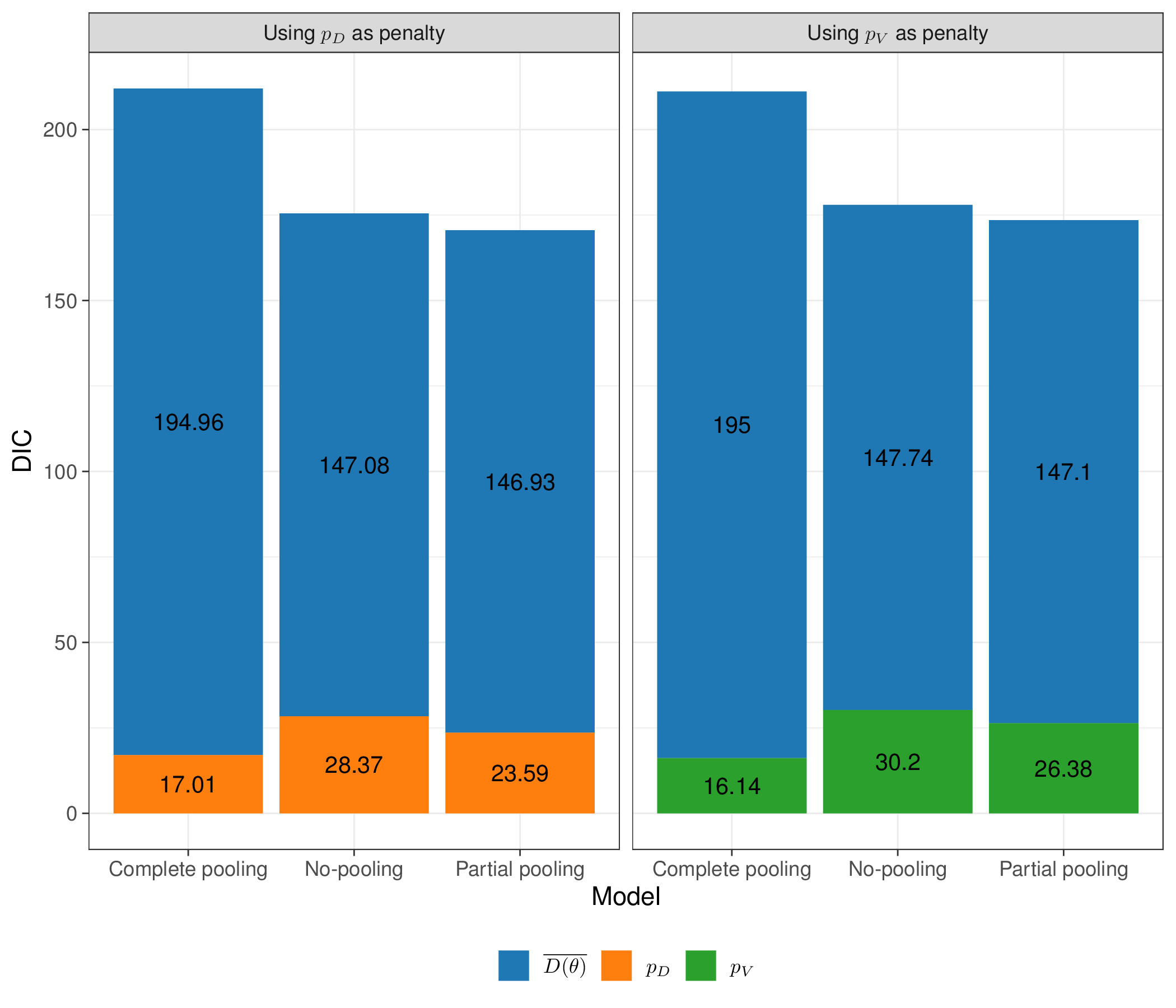
The value of \(p_D\) for the partial pooling model indicates that the effective number of parameters (23.59) is substantially lower than the nominal one (35), by effect of the implied correlation and borrowing of information among the \(\delta_s\). This is also in line with \(p_V\), as reported in Table 6.2.
Note 6.4: Model averaging
In line with the discussion in Section 5.3.5, instead of simply selecing the “best” model, we could instead use the resulting values for the DIC to combine them, in a model average-framework. We can use the following R code to determine the weights associated with each of the three versions of the model described above.
# Extracts the DIC values from the list 'model'
dic=unlist(lapply(model,function(x) x$BUGSoutput$DIC))
# Computes the absolute difference in DIC vs the model with lowest value
delta.dic=abs(min(dic)-dic)
# Computes the weights
(exp(-.5*delta.dic)/sum(exp(-.5*delta.dic))) |> format(scientific=FALSE)
no_pooling complete_pooling partial_pooling
"0.097032364701307" "0.000000005975042" "0.902967629323651" First, we extract the value of the DIC from each of the three models, stored in the list model; then we construct the values for \(\Delta\text{DIC}_h\) for each of the \(H=3\) options and then apply Equation 5.18 to compute the weights.
As is possible to see, in this case, the mixture is a bit more meaningful: the partial pooling model still drives the model average (with a weight of around 0.9); however, because the difference in DIC between the partial pooling and the complete pooling is around 4.5, in line with Figure 5.6, the latter has a non-negligible weight of around 0.1.
Table 6.3 shows some summary comparison of the complete vs partial pooling model. Interestingly, when assuming no heterogeneity in the trials, the effect of magnesium disappears – the OR is virtually 1 and the 95% interval is relatively narrow and spanning across 1. This is highly influenced by the ISIS-4 trial, which is by far the largest and with a result at odds with most of the other trials.
When allowing for the possibility of heterogeneous effects with the partial pooling model, the results change dramatically, with magnesium now being substantially protective. The posterior mean OR of death is 0.43 (i.e. an average reduction in the odds of death of around 57%) and the entire 95% interval is below 1.
| Model | OR (95% interval) | Between study sd (\(\sigma_\delta\)) | \(\overline{D(\boldsymbol\theta)}\) | \(p_D\) | DIC |
|---|---|---|---|---|---|
| Complete pooling | 1 (0.95; 1.07) | --- | 195.0 | 17.01 | 212.01 |
| Partial pooling | 0.43 (0.25; 0.64) | 0.61 (0.32; 1.03) | 147.1 | 23.59 | 170.69 |
Figure 6.14 shows an analysis of the magnesium effect across the three models. In some cases, the estimates for the log OR from the no- and partial pooling are fairly similar – that is the case for trials with large sample size. However, for those with weaker evidence (e.g. \(\delta_4\)), the no-pooling model shows much larger uncertainty. This is because the estimate is based only on that small study, while for the partial pooling model, it benefits from the information coming from the other larger studies.
As mentioned above, another interesting point is that the complete pooling model is highly influenced by ISIS-4, which is by far the largest study. The estimate for \(d\) is pooled towards the estimate for \(\delta_{16}\). However, the partial pooling model mitigates this and the posterior distribution for \(d\) is more balanced and influenced by the combined evidence present in the other 15 trials.
Finally, we also show the estimate for the predictive distribution \(\delta_{pred}\): unsurprisingly, this is more or less centred around the same mean as \(d\), but with larger variance. This is because the best estimate for a future trial is essentially given by the average of what has been observed so far – but we are more uncertain because the new study has not been observed yet.
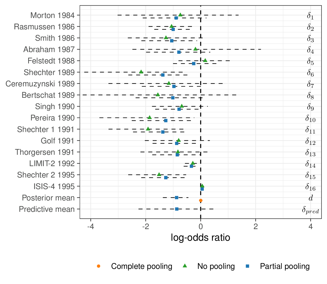
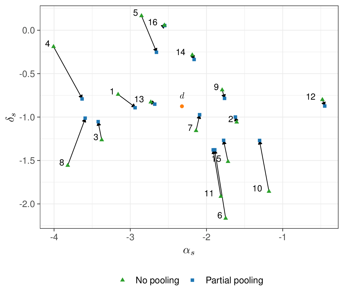
Figure 6.15 shows the amount of “shrinkage” – that is the phenomenon whereby the estimates are pulled towards the grand mean (\(d\)). Again, for smaller study, the amount of pulling is larger – it is possible to see that the arrow from the no- to the partial pooling for, say, study number 4 (which only has around 50 individuals in each arm) is much longer than for, say, study number 16 (ISIS-4), for which there is basically no difference in the two estimates.
6.3 Evidence synthesis and economic modelling
We can use the principles described above and extend the statistical modelling to the actual economic evaluation, by further combining the estimates for the model parameters so as to obtain relevant measures of population average benefit and costs.
Generally speaking, when the inputs are made by ALD, the process can be divided into the following steps. First, we build a population level model, for example using decision trees or Markov models (see Chapter 9), to represent the “natural history of the disease”. This is typically a simplified version of the underlying reality, which we use to describe how individuals may be affected by a given disease.
Again, in general terms, there is no reason why the actual data might not comprise of a combination of individual- and aggregated-level data: for instance, we may have access to a full dataset (as in Example 5.1 and throughout Chapter 5) that can inform some of the relevant parameters, but only summary statistics for others. Even more realistically, we may have access to a number of studies that we can use to inform our final estimate and then propagate the resulting uncertainty all the way to the decision process, as we demonstrate in Example 6.7.
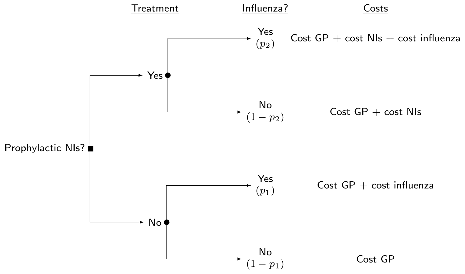
Example 6.7. Influenza (adapted and expanded from Cooper et al., 2004). Neuraminidase inhibitors (NIs) are a class of antiviral drugs that provide additional potential strategies for the control of influenza. The objective of this analysis is to build an economic model to determine the cost-effectiveness of the prophylaxis with NI, compared to a “status quo” in which no other treatment is available. Figure 6.16 shows a decision tree, in which we assume that the only relevant uncertainty is about whether people can be infected by influenza or not. Depending on the treatment that they are given, this happens with different probabilities (say, \(p_2\) under the active treatment arm, or \(p_1\), in case the prophylaxis is not applied/available).
In reality, the underlying clinical pathways may be much more complicated – for instance, here, we do not consider complications, other adverse events, etc., but, in line with Cooper et al. (2004), do limit the analysis to this much simplified version of the problem.
Evidence synthesis for the relative effectiveness of NIs
Cooper et al. (2004) consider a number of \(S=6\) randomised trials comparing the use of NIs against no prophylaxis to reduce the incidence of influenza (specifically the A and B types) during an epidemic.
The data are shown in Table 6.4 and can be modelled in a similar way to the ones used in Example 6.1, i.e. \(r_{st}\sim\text{Binomial}(\pi_{st},n_{st})\), for \(s=1,\ldots,S=6\) studies and \(t=1,2\) treatment arms. The linear predictor is modelled as \[ \text{logit}(\pi_{s1}) = \alpha_{s} \qquad \mbox{and} \qquad \text{logit}(\pi_{s2}) = \alpha_s + \delta_s, \] where \(\alpha_s\) is a study-specific log event (i.e. baseline risk of influenza) rate in the placebo group, while \(\delta_s\) is the study-specific log OR, quantifying the effect of the prophylaxis.
| Placebo | NIs | ||||
|---|---|---|---|---|---|
| Study | Age group | Total \(n_1\) | Cases \(r_1\) | Total \(n_2\) | Cases \(r_2\) |
| Monto et al. (1999) | 18-64 | 554 | 34 | 553 | 11 |
| Hayden et al. (2000) | 5+ | 423 | 40 | 414 | 7 |
| Kaiser et al. (2000) | 13-65 | 144 | 9 | 144 | 3 |
| Hayden et al. (1999) | 18-65 | 268 | 19 | 268 | 3 |
| Hayden et al. (1999) | 18-65 | 251 | 6 | 252 | 3 |
| Welliver et al. (2001) | 12-85 | 462 | 34 | 493 | 4 |
We slightly modify the original analysis in Cooper et al. (2004) and complete our evidence synthesis model with the following assumptions: \[ \begin{aligned} \alpha_s & \sim \text{Normal}(0,\text{sd}=10) \\ \delta_s & \sim\text{Normal}(\mu_\delta,\sigma_\delta) \\ \mu_\delta & \sim \text{Normal}(0,\text{sd}=10) \\ \sigma_\delta & \sim \text{Exponential}(\lambda_\delta). \end{aligned} \] In this specification, the baseline risk \(\alpha_s\) are modelled independently (no-pooling), while the treatment effect \(\delta_s\) is modelled using partial pooling; thus, \(\text{OR}=\exp\left(\mu_\delta\right)\) represents the pooled OR overall relative treatment effect.
Evidence synthesis for the underlying probability of influenza in the adult population
In addition to the \(S\) head-to-head comparisons for NIs vs placebo, there are data from \(H=9\) randomised studies in which the control arm (placebo) can be used to measure the incidence of influenza among healthy adults, in terms of number of observed cases \(\boldsymbol{y}=(y_1,\ldots,y_H)=(0,6,5,6,25,18,14,3,27)\) over the total sample size \(\boldsymbol{m}=(m_1,\ldots,m_H)=(23,241,159,137,519,298,137,24,132)\).
Again, we slightly modify the model originally presented in Cooper et al. (2004) and assume \(y_h\sim\text{Binomial}(\theta_h,m_h)\) with \[ \begin{aligned} \text{logit}(\theta_h) & = \beta_h \sim\text{Normal}(\mu_\beta,\sigma_\beta)\\ \mu_\beta & \sim \text{Normal}(0,\text{sd}=10) \\ \sigma^2_\beta & \sim\text{Exponential}(\lambda_\beta). \end{aligned} \]
Rescaling \(\mu_\beta\) allows us to obtain an estimate of the pooled baseline probability of influenza infection for a random individual of the general population, i.e. in case no treatment is available, i.e. \[ p_1 = \frac{\exp(\mu_\beta)}{1+\exp(\mu_\beta)} \quad \Leftrightarrow \quad \text{logit}(p_1) = \mu_\beta. \]
NotePooling all background information
In the model described above, the parameters \(\alpha_s\) and \(\beta_h\) are modelled as two separate and independent processes: in the case of the baseline risks for the \(S\) head-to-head studies, we apply no-pooling, while we pool together the other \(H\) studies to estimate the background probability of influenza \(p_1=\text{logit}^{-1}(\mu_\beta)\).
We could use a slightly different version of the model, in which also the baseline risk \(\alpha_s\) are modelled using partial pooling across the \(S\) studies, which could be achieved by assuming the following structure \[ \begin{aligned} \alpha_s & \sim \text{Normal}(\mu_\alpha,\sigma_\alpha) \\ \mu_\alpha & \sim \text{Normal}(0,\text{sd}=10) \\ \sigma_\alpha & \sim \text{Exponential}(\lambda_\alpha). \end{aligned} \] In this case, we would also estimate a pooled background risk of influenza (\(\mu_\alpha\)). This specification would relax the original assumption that the \(S\) head-to-head studies are effectively too heterogeneous in their definition of the placebo arm (and hence not pooled at all), while allowing for some shrinkage in the estimates for the \(\alpha_s\) parameters. Even in this case, however, the parameters \(\alpha_s\) and \(\beta_h\) would be modelled separately.
On the one hand, this separation may be justified, for instance if we think that there may be strict inclusion criteria for the \(S\) head-to-head studies that perhaps do not really match those that characterise the \(H\) studies from which we gather evidence to estimate the baseline probability \(p_1\). Perhaps, the head-to-head studies are very specific and therefore we do not want to use them to inform a parameter that is supposed to work at the general population level.
On the other hand, we may in fact think that, in reality, the \((S+H)\) studies are all fairly similar, at least in their definition of the placebo arm and, if that is the case, we may be willing to actually model \(\alpha_s\) and \(\beta_h\) as exchangeable – in other words to assume that they have a common data-generating process, e.g. \[ \alpha_s,\beta_h \sim \text{Normal}(\mu_\beta,\sigma_\beta). \]
If this assumption is reasonable, we would probably gain some precision in the resulting estimate for \(p_2\), because it would be based on a larger number of data points. Of course, if the two sets of studies are actually quite heterogeneous, we may not be willing to assume exchangeability among the main parameters and be better off modelling them separately (although as exchangeable within the two modules).
We can combine the two modules and apply the estimated treatment effect (OR) from the first evidence synthesis to the baseline probability \(p_1\), estimated in the second module. As by definition the OR is the ratio of two probability odds, e.g. \(\displaystyle \frac{p_2}{1-p_2} = \text{OR}\frac{p_1}{1-p_1}\), then taking logs on both sides we obtain \[ \begin{aligned} \text{logit}(p_2) = \log\left(\frac{p_2}{1-p_2}\right) & = \log\left(\text{OR}\frac{p_1}{1-p_1}\right) \\ & = \log\text{OR}+ \log\left(\frac{p_1}{1-p_1}\right) \\ & = \log\text{OR}+ \text{logit}(p_1). \end{aligned} \] In a Bayesian context, this of course means that we propagate the uncertainty in the estimates for OR and \(p_1\) all the way to the implied posterior distribution for \(p_2\).
NoteBaseline-risk adjustment
The original model in Cooper et al. (2004) considers a slightly different structure for the evidence synthesis on the \(S\) head-to-head trials, where the linear predictor for the treatment arm is \[ \text{logit}(\pi_{s2})=\alpha_s + \delta^*_s + \gamma(\alpha_s-\bar{\alpha}). \] In this formulation, the study-specific log OR is then \(\delta_s = \delta^*_s + \gamma(\alpha_s + \bar{\alpha})\), where \(\delta^*_s\sim\text{Normal}(\mu_\delta,\sigma_\delta)\) is a study-specific treatment effect, while \(\gamma(\alpha_s-\bar{\alpha})\) is used to adjust for differences in the study-specific background risk. In this model, \(\mu_\delta\) is the pooled treatment effect – this is obtained for a hypothetical study in which the baseline risk is identical to the underlying average and thus the term \((\alpha_s-\bar{\alpha})\) is 0.
While, in general, this adjustment may be important and reduce bias (Welton et al., 2012, pp. 107–109), when the underlying data are reasonably consistent, there may not be any material difference, in practice.
Cost and benefit parameters
Following Cooper et al. (2004), we consider that the course of prophylaxis assumes 6 weeks of daily treatment at a cost of £2.4 per day and thus, assuming VAT at 17.5%, a total \(c^{\rm{\it NI}}=\) £118.44, as well as a fixed cost \(c^{\rm{\it GP}}=\) £19 for a GP visit. As indicated in Figure 6.16 and in line with the original analysis in Cooper et al. (2004), we assume that even in the case where NIs are not prescribed, there is a background GP visit (and hence a cost of \(c^{\rm{\it GP}}\) even in the bottom branch of the decision tree).
As for the cost of treating a case of influenza (including GP visits, outpatient visits and inpatient stays but not time off work, for adults), we should account for the individual variance. Official resource use data suggest that the average total cost is £16.78 and a standard deviation of £2.34. We can use these values to define an informative prior to model the total cost of treatment for influenza, for example using \(c^{\rm{\it Inf}}\sim\text{Normal}(\text{mean}=16.78,\text{sd}=2.34)\).
Technically, the Normal distribution is not the most appropriate for a quantity that must be positive, but given the values for the mean and standard deviation, the chance of this quantity being negative is effectively non-existent – and to be precise, this can be computed as pnorm(0,16.78,2.34)=0, which for all intents and purposes is 0.
The final element included in the model is the average duration of the influenza infection. Cooper et al. (2004) models this as \(l\sim\text{log-Normal}(\mu_l,\sigma_l)\), where the mean and standard deviation \((\mu_l,\sigma_l)\) are selected so that on the natural scale the mean is 8.2 and the standard deviation is 2 days. We can use the function lognPar() from the package bmhe to map the natural scale values to the log scale
mu.l=bmhe::lognPar(8.2,2)$mulog
sigma.l=bmhe::lognPar(8.2,2)$sigmalog
and the resulting values are computed at \(\mu_l = 2.0752411\) and \(\sigma_l = 0.2403875\).
JAGS modelling and analysis
The modelling assumptions described above can be embedded in the code listed below. Notice that we use a PC prior \(\text{Exponential}(1.65)\) for all the standard deviations of the structured effects \(\alpha_s\), \(\beta_h\) and \(\delta_s\), to imply \(\Pr(\sigma_\alpha>1)=\Pr(\sigma_\beta>1)=\Pr(\sigma_\delta>1)\approx 0.2\) (see Section 2.2.3). In line with the discussion of Section 6.2.5, we avoid the use of the \(\text{Gamma}(0.001,0.001)\) for the various precisions \(\tau_\delta\), which was used in the original model of Cooper et al. (2004)
Another difference in our setup is for the prior selected for \(\mu_\beta\), which in the original formulation has a very large value for the standard deviation (1 000 000). We change this too to a value of 10 – the underlying parameter is modelled on the logit scale and a standard deviation of 10 still implies a very large variance, when rescaled to the probability range \([0;1]\).
influenza=function() {
  # 1. Evidence synthesis of relative effectiveness vs placebo
  for (s in 1:S) {
    # Placebo arm
    r1[s] ~ dbin(pi1[s],n1[s])
    logit(pi1[s]) <- alpha[s]
    # NIs arm
    r2[s] ~ dbin(pi2[s],n2[s])
    logit(pi2[s]) <- alpha[s] + delta[s]
    # Study-specific baseline probability of influenza (logit scale)
    alpha[s] ~ dnorm(0,0.1)
    # Study-specific log-OR for NIs
    delta[s] ~ dnorm(mu.delta,tau.delta)
  }
  # Pooled log-OR for NIs vs placebo
  mu.delta ~ dnorm(0,0.1)
  # Prior on the sd of delta[s]
  sigma.delta ~ dexp(1.65);  tau.delta <- pow(sigma.delta,-2)
  # Pooled log-OR for NI vs placebo
  or <- exp(mu.delta)

  # 2. Evidence synthesis for incidence of influenza
  for (h in 1:H) {
    y[h] ~ dbin(theta[h],m[h])
    logit(theta[h]) <- beta[h]
    beta[h] ~ dnorm(mu.beta,tau.beta)
  }
  # Pooled influenza incidence among adults (with no NIs) on the logit scale
  mu.beta ~ dnorm(0,0.1)
  # Prior on the sd of beta[h]
  sigma.beta ~ dexp(1.65);   tau.beta <- pow(sigma.beta,-2)

  # 3. Probability of influenza with and without NIs
  # Rescaled pooled probability of influenza without NIs
  logit(p1) <- mu.beta
  # Rescaled probability of influenza with NIs
  logit(p2) <- logit(p1) + mu.delta

  # 4. Outcomes
  # Model for the costs of treating influenza (prec = 1/2.34^2 = 0.1826)
  c.inf ~ dnorm(16.78,0.1826)
  # Duration of infection (prec = 1/0.2403^2 = 17.3051)
  l ~ dlnorm(2.075,17.3051)
}
We can then construct a data list using the values in Table 6.4 and for the variables \(\boldsymbol{y}\), \(\boldsymbol{m}\), \(H\) and \(S\) and then call the function jags() to run the model and save the output in the object flu, say. We use 25 000 iterations, with a burn-in of 5000 and thinning of 1 every 10 iterations, to limit the potential impact of autocorrelation.
The resulting estimates are shown in the table below.
Inference for Bugs model at "/tmp/RtmpIMtjqt/modelffaea41801e97.txt",
 2 chains, each with 25000 iterations (first 5000 discarded), n.thin = 10
 n.sims = 4000 iterations saved. Running time = 0.816 secs
         mu.vect sd.vect   2.5%    25%     50%     75%   97.5%  Rhat n.eff
c.inf     16.774   2.388 12.126 15.168  16.766  18.368  21.431 1.001  4000
l          8.224   1.991  5.030  6.784   7.954   9.390  12.863 1.001  4000
or         0.208   0.060  0.117  0.171   0.202   0.238   0.331 1.002  1600
p1         0.061   0.018  0.033  0.049   0.059   0.071   0.103 1.001  2400
p2         0.014   0.006  0.006  0.010   0.012   0.016   0.027 1.001  4000
deviance 102.840   5.976 92.762 98.621 102.311 106.417 116.341 1.001  4000

For each parameter, n.eff is a crude measure of effective sample size,
and Rhat is the potential scale reduction factor (at convergence, Rhat=1).

DIC info (using the rule: pV = var(deviance)/2)
pV = 17.9 and DIC = 120.7
DIC info (using the rule: pD = Dbar-Dhat, computed via 'rjags::dic.samples')
pD = 15.9 and DIC = 118.8
DIC is an estimate of expected predictive error (lower deviance is better).
The diagnostic measures are satisfactory for all the major nodes included in the analysis. In particular, we see that the baseline pooled probability of influenza is estimated at 0.061 with a 95% posterior interval \([0.033; 0.103]\), whereas the probability of infection in the NIs prophylaxis arm is estimated at a much lower value 0.014 with a 95% posterior interval \([0.006; 0.027]\).
We can also run the version of the model in which \(\alpha_s\) and \(\beta_h\) are modelled as exchangeable (i.e. pooling together all the information on the background risk of influenza) – this is easy to do by simply ensuring that the two sets of parameters have the same data-generating process, e.g. by modifying the code above to alpha[s] ~ dnorm(mu.beta,tau.beta). Figure 6.17 shows a comparison of the results for the main model parameters (\(p_1,p_2,\text{OR}\)).
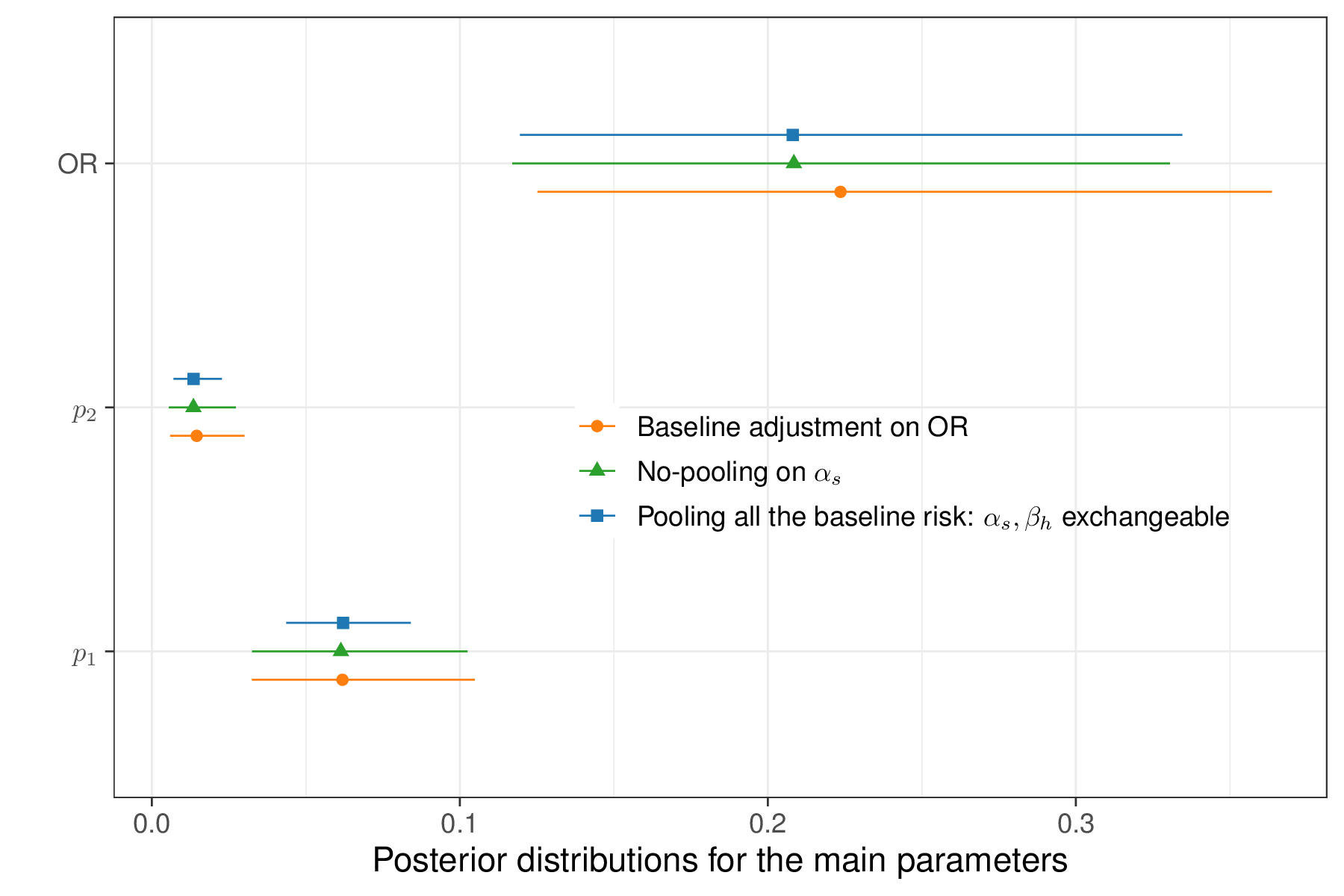
As is possible to see, in this particular case, the two versions of the model do not differ substantially. The model pooling all the available information in the background risk of influenza (labelled as “\(\alpha_s,\beta_h\) exchangeable” in Figure 6.17) tends to produce slightly more precise estimates for \(p_1\). This is due to the fact that the two sets of studies are indeed probably quite comparable. Conversely, the estimates for the OR are slightly more variable in the base-case analysis where \(\alpha_s\) and \(\beta_h\) are not pooled together, but they are still fairly aligned.
Figure 6.17 also displays the results for the model adjusting for the baseline risk in the \(S\) head-to-head studies – in this case, the posterior distribution for the OR is shifted to the right, with a slightly larger average value. However, these differences do not appear material, which is consistent with the fact that a posterior 95% interval of \([-2.14;0.56]\) is estimated for the parameter \(\gamma\); as it spans across 0, this indicates that the effect of the baseline adjustment is “non-significant”.
Even in terms of model fitting, the three versions described here have very minimal differences: in terms of DIC, the computed values are 118.8, 117.9 and 117.7 for the base-case, pooling for all the baseline risk and baseline risk adjustment versions.
Post-processing and economic evaluation
In order to fully quantify the costs and benefits of the two alternative strategies, we need to also consider further quantities. Assuming that \(l\) is the length of the influenza infection, \(c^{\rm{\it GP}}\) is the cost of a preliminary GP visit to issue the prescription of NIs, \(c^{\rm{\it NI}}\) is the total cost for the prophylactic NIs and \(c^{\rm{\it Inf}}\) is the cost of treating influenza, given the structure of the problem described in Figure 6.16, the population average outcomes are: \[ \mu_{e1}=-lp_1 \qquad \mbox{and} \qquad \mu_{e2}=-lp_2 \tag{6.11}\] for the clinical effectiveness, which we simplistically measure here as “the number of days required to clear the infection”, without any specific reference to utilities1 (with longer duration being worse – hence the negative sign); and \[ \begin{aligned} \mu_{c1}& =(1-p_1)c^{\rm{\it GP}} + p_1\left( c^{\rm{\it GP}} + c^{\rm{\it Inf}} \right) \\ \mu_{c2}& =(1-p_2)\left( c^{\rm{\it GP}} + c^{\rm{\it NI}} \right) + p_2 \left( c^{\rm{\it GP}} + c^{\rm{\it Inf}} + c^{\rm{\it NI}} \right), \end{aligned} \tag{6.12}\] for the costs – it is easy to follow the pathways in the decision tree of Figure 6.16 and work out what the resulting cost would be overall.
We can post-process the output of the Bayesian modelling to construct the main economic summaries, as defined in Equations 6.11 and 6.12, using the following R code
# Define the variables 'mu.e' and 'mu.c' as empty matrices with 'n.sims'
# rows (one per each MCMC simulation) and 2 columns (one per treatment arm)
n.sims=flu$BUGSoutput$n.sims
mu.e=mu.c=matrix(NA,n.sims,2)

# Fixed costs
# Cost of GP visit to issue NIs prescription
c.gp=19
# Cost of course of treatment with NIs
c.ni=2.40*6*7*1.175

# Extracts simulations from the object 'flu' (for simplicity in the code)
p1=flu$BUGSoutput$sims.list$p1
p2=flu$BUGSoutput$sims.list$p2
c.inf=flu$BUGSoutput$sims.list$c.inf
l=flu$BUGSoutput$sims.list$l

# Population average costs
mu.c[,1]=(1-p1)*c.gp + p1*(c.gp+c.inf)
mu.c[,2]=(1-p2)*(c.gp+c.ni) + p2*(c.gp+c.ni+c.inf)

# Population average effects
mu.e[,1]=-l*p1
mu.e[,2]=-l*p2

# Now uses 'BCEA' to make the economic analysis
m=bcea(mu.e,mu.c,interventions=c("Status quo","NIs prophylaxis"),ref=2)
# Economic analysis
summary(m,wtp=1000)
Cost-effectiveness analysis summary

Reference intervention:  NIs prophylaxis
Comparator intervention: Status quo

Optimal decision: choose Status quo for k < 300 and NIs prophylaxis for k >= 300


Analysis for willingness to pay parameter k = 1000

                Expected net benefit
Status quo                   -524.29
NIs prophylaxis              -248.48

                                 EIB    CEAC   ICER
NIs prophylaxis vs Status quo 275.81 0.99625 298.99

Optimal intervention (max expected net benefit) for k = 1000: NIs prophylaxis

EVPI 0.12583
As is possible to see from the BCEA output, the ICER is very small – around £299 and thus prophylaxis is a very cost-effective strategy, even for very small willingness to pay. We can also use the simulations from our model to summarise directly the differential costs and benefits.
Interestingly, the benefits in terms of number of days with influenza avoided are concentrated to a relatively small number – Figure 6.18 shows a histogram for the posterior distribution of the population average difference \(\Delta_e=(\mu_{e2}-\mu_{e1})\), as well as the empirical cumulative distribution function (ecdf).
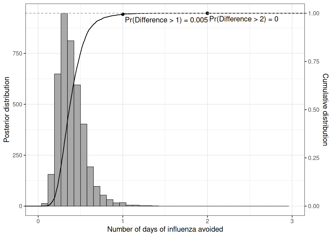
We can read the probability that the benefits exceed a given threshold along the \(x-\)axis directly off the ecdf; for instance, the chance of more than 1 day of influenza avoided is only around 1% – this can be computed as \(\Pr(\Delta_e>1) = 1-F_{\Delta_e}(1)\), i.e. the difference between 1 and the ecdf computed for 1.
6.4 Conclusions
This chapter has presented the principles of hierarchical modelling as a compromise between the extreme situations: one in which the data are distinctly heterogenous and therefore should not be pulled together and another in which, on the contrary, we can reasonably assume a single data-generating process, characterised by a single common (set of) parameters, which are then estimated with larger precision because all the information can be pulled together.
These models and a deeper understanding of when each may be appropriate, are the cornerstone of the almost ubiquitous process of “evidence synthesis”, which is very prevalent in HTA applications, especially when individual-level data are not directly available (e.g. for reasons due to confidentiality in clinical experimentation) and therefore the analysis is based on connecting various summary statistics.
The next chapter expands on these concepts to consider multiparameter evidence synthesis as well as situations in which the complex nature of the available data include the necessity of “filling the gaps” in a network of evidence for which specific pairwise comparisons are not directly observed.
While this is not ideal, it will not be too complicated to find estimates of the utility associated with having influenza↩︎