# Load the package - assuming it's been installed (check https://gianluca.statistica.it/software/survhe/ for guidance)
library(survHE)

# Loads the fictional dataset
data("survtrial")

# Turns the dataset into a "tibble" object and then inspects it
data=data %>% as_tibble()
data
## # A tibble: 367 × 8
##    ID_patient  time censored   arm   sex   age   imd ethnic
##         <int> <dbl>    <int> <int> <int> <int> <int>  <int>
##  1          1  0.03        0     0     1    34     1      4
##  2          2  0.03        0     0     0    29     4      2
##  3          3  0.92        0     0     0    30     4      5
##  4          4  1.48        0     0     0    31     5      1
##  5          5  1.64        0     0     0    27     4      1
##  6          6  1.64        0     0     0    37     5      4
##  7          7  1.7         0     0     0    31     2      5
##  8          8  1.7         0     0     1    30     2      4
##  9          9  1.74        0     0     0    40     3      5
## 10         10  1.77        0     0     0    34     3      3
## # ℹ 357 more rowsA (quick) tutorial on how to use survHE for survival modelling in health economics
survHE
Bayesian statistics
Health economics
This tutorial is based on the Journal of Statistical Software paper describing the philosophy underlying survHE and its main functionality. All the technical details (including the statistical background) are described in the paper, while this tutorial is only meant to provide some annotated description of the main important functions provided in survHE.
The example uses a fictional dataset — in fact the actual data are created by “digitising” an existing Kaplan Meier curve. survHE is based on the output produced by DigitizeIt, but there are other possibilities — and in the future we plan on including different sources for pre- and post-processing from within survHE.
The current version of survHE uses modern R tools and packages for data management and programming (based on the tidyverse). Thus when survHE is loaded in the R workspace, relevant functions from dplyr and “piping” (%>%) are immediately available for the user.
As a first example, we run a survival model using a few distributional assumptions. The main survHE function is fit.models, which can be used to specify:
- the model “formula”, which describes the relationships between the observed data and (potentially) relevant covariates;
- the data, which are used to estimate the model parameters and the relevant survival quantities (including the survival curves);
- the distribution to be used to approximate sampling variability for the outcome;
- the method that should be used to fit the model.
Survival modelling using Maximum Likelihood Estimators
A typical call to fit.models is like the following.
# First, defines the vector of models to be used
mods <- c("exp", "weibull", "gamma", "lnorm", "llogis", "gengamma")

# Then the formula specifying the linear predictor
formula <- Surv(time, censored) ~ as.factor(arm)

# And then runs the models using MLE via flexsurv
m1 <- fit.models(formula = formula, data = data, distr = mods)
Here, we are considering 6 different parametric distributions: Exponential, Weibull, Gamma, log-Normal, log-Logistic and Generalised Gamma. Because we’re specifying the value for the argument distr in a vector (with the 6 models), fit.models will store the results for all of them into a single object (in this case, m1). This is not necessary and alternatively, we can use a separate call to fit.models for each distributional assumption.
The model specified in the object formula essentially assumes the following specification. \[\begin{eqnarray*}
t_i & \sim & f(t_i \mid \boldsymbol\theta) \\
\boldsymbol\theta & = & (\mu, \alpha) \\
g(\mu_i) & = & \beta_0 + \beta_1 \mbox{Arm}_i.
\end{eqnarray*}\] Here, \(f(t_i \mid \boldsymbol\theta)\) is the density function associated with each of the 6 models specified; \(\boldsymbol\theta = (\mu, \alpha)\) is a vector of model parameters, including a location parameter \(\mu\) and a (set of) ancillary parameters \(\alpha\), indicating a measure of shape or variance for the underlying distribution. Moreover, we assume a generalised linear regression on the location parameter (based on a suitable link function \(g(\cdot)\), typically, the \(\log\)), which is based on an intercept \(\beta_0\) and a single covariate \(\mbox{Arm}_i,\) whose effect is quantified by the coefficient \(\beta_1\). Notice that because the formula specifies as.factor(arm), we essentially consider this as a categorical variable — taking values 0 for the controls and 1 for the individuals in the treatment arm.
In the R formula, we need to specify not only the observed outcome (in this case \(t=\) time), but also the censoring indicator (in this case \(d=\) censored). This is crucial in the context of survival modelling.
Survival modelling using Integrated Nested Laplace Approximation
For several reasons (many of which you would expect from me…), it is often useful to be Bayesians about modelling, particularly if the overarching objective is to feed the output of the statistical building block to an economic model and, downstream, to a decision-making process.
survHE uses two Bayesian inferential engine (section 2.3 of the paper explains why). The first one is Integrated Nested Laplace Approximation (INLA), which is a very efficient way of obtaining estimates from the marginal posterior distributions of the model parameters. While INLA currently fits only 4 parametric survival models, it is generally as fast as the MLE counterparts.
In survHE, the user can specify that they want to use INLA by simply adding an option method="inla" to the call to fit.models, something like the following.
# Runs the models using INLA using the formula and data specified above, but with the subset of distributions that INLA can fit
m2 <- fit.models(formula = formula, data = data, distr = c("exp","wei","lno","llo"), method="inla")
Survival modelling using Hamiltonian Monte Carlo
Markov Chain Monte Carlo (MCMC) methods are arguably the default mode of fitting Bayesian models. Software such as BUGS, JAGS, Nimble and, more recently, Stan all implement some MCMC algorithm to obtain samples from the posterior joint distribution of all the model parameters. In particular, rstan uses a version of MCMC, called Hamiltonian Monte Carlo (HMC), which can be very efficient in exploring the posterior distribution.
survHE implements rstan versions of all the parametric models described in the paper (which are recommended by NICE). Similarly to INLA, all the user needs to add is the option method="hmc" to instruct fit.models to run rstan in the background.
# Runs the models using HMC using the formula and data specified above
m3 <- fit.models(formula = formula, data = data, distr = mods, method="hmc")
Several more options are described in details in the survHE paper.
Printing and plotting with survHE
survHE is meant to simplify the workflow for health economic modellers by standardising the process (e.g. through a common and simplified call to define the models to be fitted, as shown above). To this aim, it comes with “methods” that can be deployed for survHE objects (such as m1, m2 and m3 created by the code above), to summarise and visualise the process.
These methods take the output created by either flexsurv, INLA or rstan and format it in a standardised way that the modellers can use to feed into the economic model. For instance, we can summarise the model coefficients using the print method.
# Prints the output of the three objects (by default shows the first of the models stored in the survHE objects)
print(m1)
##
## Model fit for the Exponential model, obtained using Flexsurvreg
## (Maximum Likelihood Estimate). Running time: 0.016 seconds
##
##                       mean         se       L95%      U95%
## rate             0.0824203 0.00828355  0.0676839  0.100365
## as.factor(arm)1 -0.4656075 0.15427132 -0.7679738 -0.163241
##
## Model fitting summaries
## Akaike Information Criterion (AIC)....: 1274.576
## Bayesian Information Criterion (BIC)..: 1282.387

print(m2)
##
## Model fit for the Exponential model, obtained using INLA (Bayesian inference via
## Integrated Nested Laplace Approximation). Running time: 0.47367 seconds
##
##                       mean         se       L95%       U95%
## rate             0.0824172 0.00842115  0.0674624  0.0999213
## as.factor(arm)1 -0.4676212 0.15225249 -0.7761718 -0.1836731
##
## Model fitting summaries
## Akaike Information Criterion (AIC)....: 1276.580
## Bayesian Information Criterion (BIC)..: 1288.296
## Deviance Information Criterion (DIC)..: 1278.222

print(m3)
##
## Model fit for the Exponential model, obtained using Stan (Bayesian inference via
## Hamiltonian Monte Carlo). Running time: 0.670 seconds
##
##                       mean         se       L95%       U95%
## rate             0.0826441 0.00827033  0.0667495  0.0991229
## as.factor(arm)1 -0.4706873 0.15763294 -0.7749507 -0.1677673
##
## Model fitting summaries
## Akaike Information Criterion (AIC)....: 1276.579
## Bayesian Information Criterion (BIC)..: 1288.295
## Deviance Information Criterion (DIC)..: 1274.576
In this case, we have not specified much information in the prior distributions for the Bayesian versions of the models. In addition, the dataset is relatively “mature” (i.e. there are not very many censored cases) and thus the estimates for the model parameters are fairly similar in all three models. NB: this is not guaranteed in all circumstances. In fact, it is absolutely possible that, particularly in the presence of data subject to a large proportion of censored individuals (as is often the case e.g. in immuno-oncology), genuine prior information may be crucial and instrumental to producing sensible estimates!
survHE offers various options in the call to the print method. For example, we can visualise the output in the “native” formatting, i.e. that produced by the package that has been used to run the analysis. This can be obtained by adding the option original=TRUE in the call to print. However, the point of using survHE is in fact to have the output in a standardised format, so as to avoid confusion (e.g. when different software presents data and estimates using different names or terminology). In addition, when the underlying survHE object contains more than one model, the call to print automatically generates the summary statistics for the first one (in this case, the Exponential model, as this is the first to be specified in the vector mods or in the call to fit.models for m2). However, we can select any one of the models by adding the option mods=..., for instance
Perhaps even more interestingly, health economic modellers will be likely interested (almost exclusively) in the survival curves obtained from the fitted models. The user can visually inspect the models in terms of the survival curves, using the plot method.
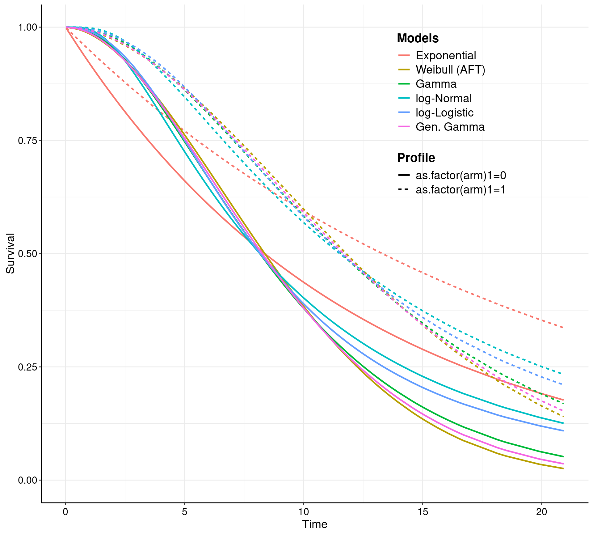
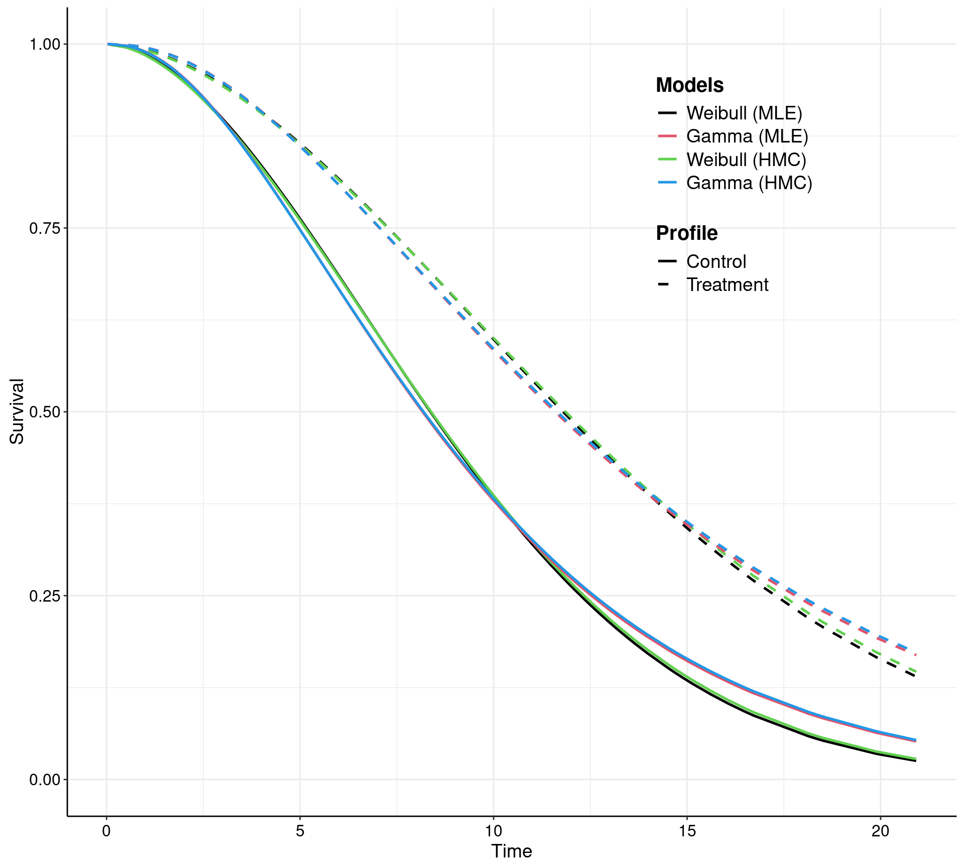
The current (and future!) version(s) of survHE use the plotting capabilities of ggplot2. As such, all graphs generated by survHE are in fact ggplot2 objects and thus they can be manipulated and post-processed at will. The expert user can customise the graphs in essentially any way they want. The less-expert users don’t actually need to do much and survHE does allow some customisation — for example, the call above specifies the options lab.model, which tells survHE what labels to use to describe the various models being depicted; and the option lab.profile, which defines specific labels for the individual “profiles” (i.e. the combination of the covariates). More options are described in the survHE paper and we will produce more tutorials (in fact, please do contribute your survHE examples, if you can — you can do so by opening “issues” on the GitHub repository or by sending me an email).
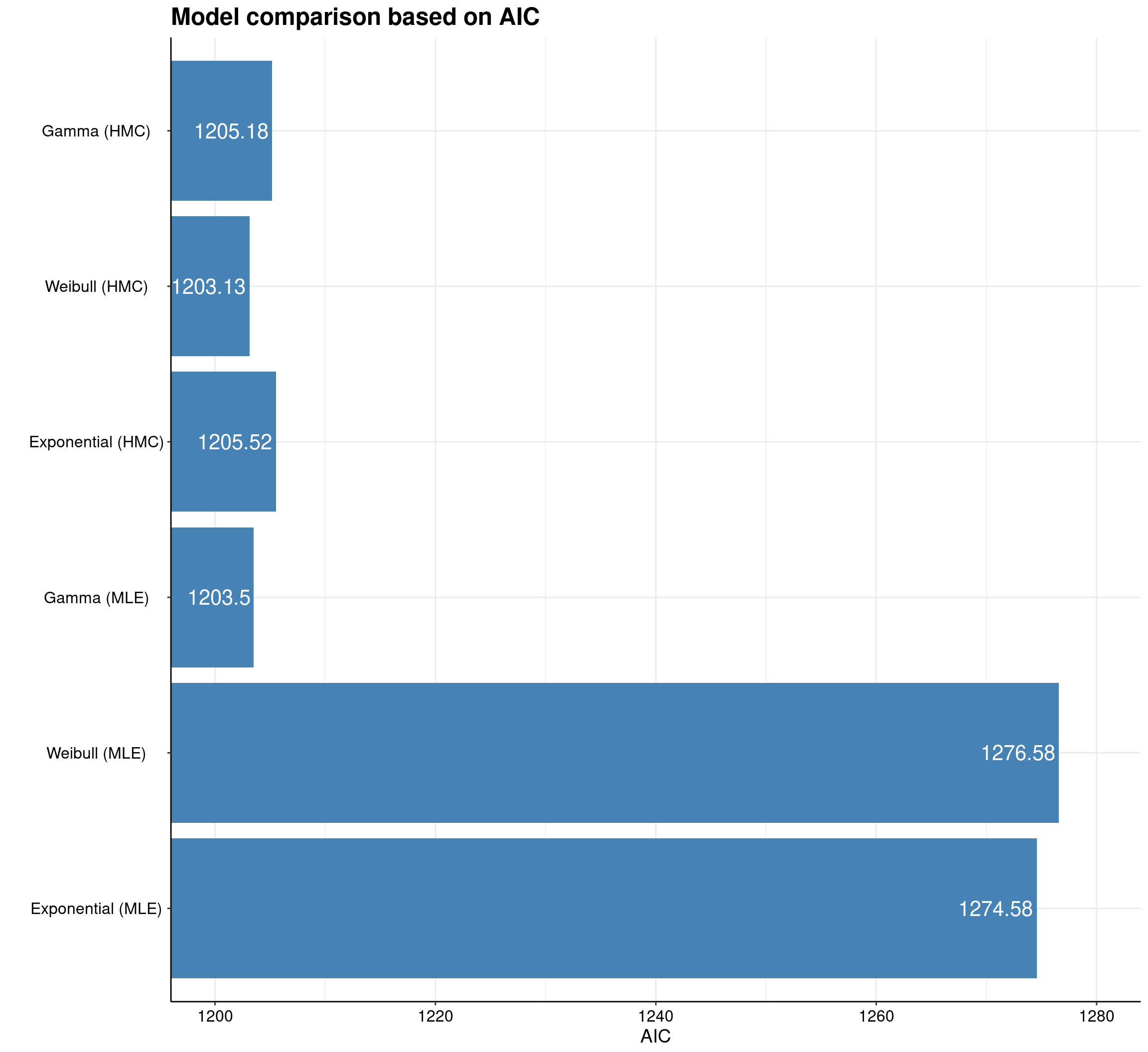
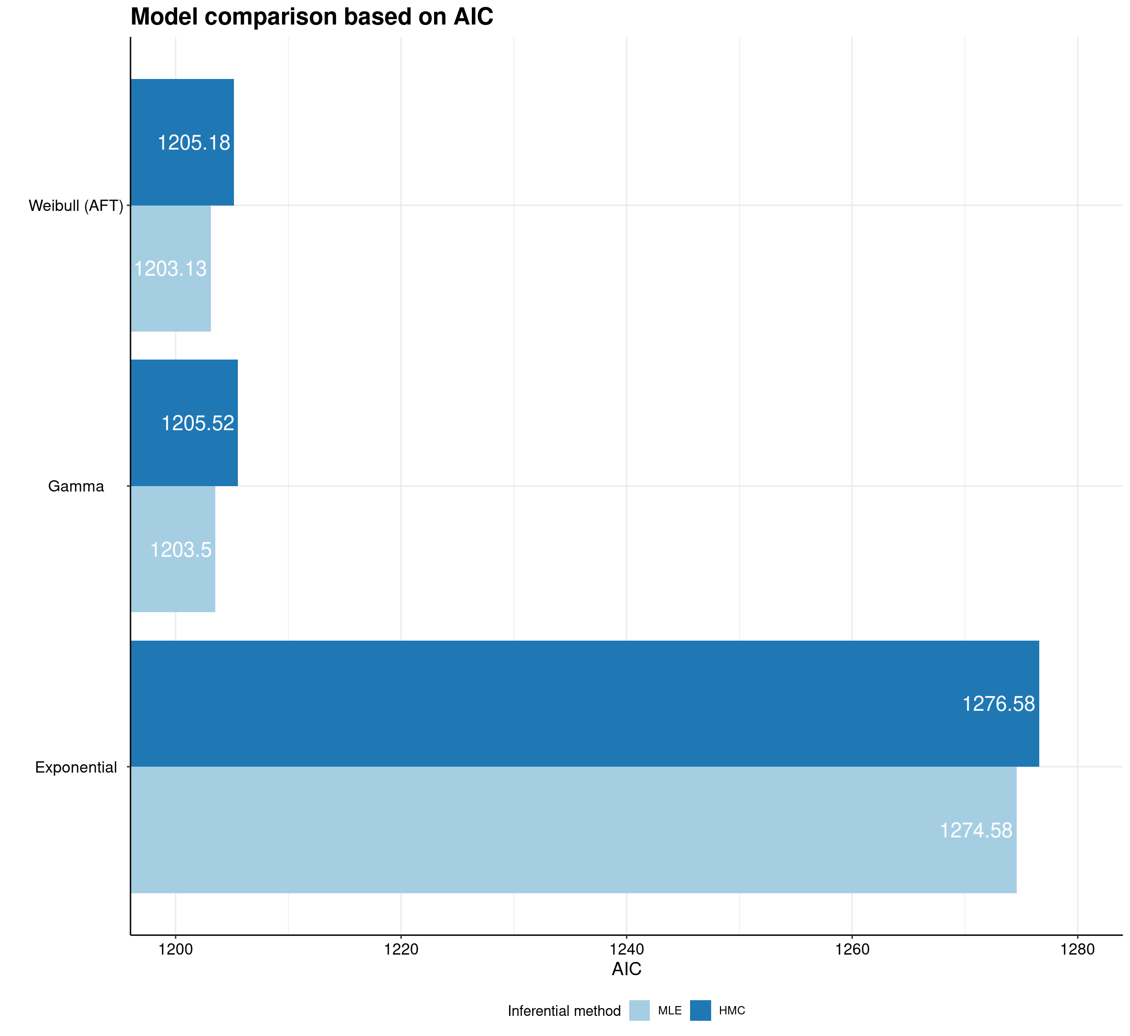
One example of ggplot2 potential is given in survHE by the model.fit.plot function, which depicts graphically the measures of model fit, based on information criteria.
Probabilistic sensitivity analysis with survHE
One of the crucial features of a health economic evaluation is represented by the need of performing probabilistic sensitivity analysis (PSA). This is one of my obsessions and I think one of the places where being Bayesian becomes natural and thus the preferred option, particularly when the end product is to use the statistical model for the purposes of an economic evaluation.
survHE has a dedicated function, make.surv that does the process of PSA in the context of the survival models. In this case, the idea is to propagate the uncertainty in the model parameters (e.g. \(\boldsymbol\beta=(\beta_0,\beta_1)\) in the current example) all the way to the elements that feed into the economic model (which typically are the survival curves for the different interventions).
In reality, the user may not even need to worry too much about how make.surv works — more advanced and statistically sophisticated modellers may use all the flexibility and power of this function to obtain a characterisation of the uncertainty underlying the model estimates (this is based on bootstrap for the MLE implementation and on samples from the posterior in the Bayesian versions). In any case, survHE also has plotting capabilities to visualise the PSA output. This can be done by going through make.surv and then applying the specialised plotting method psa.plot, or directly using the general plot method with some suitable options.
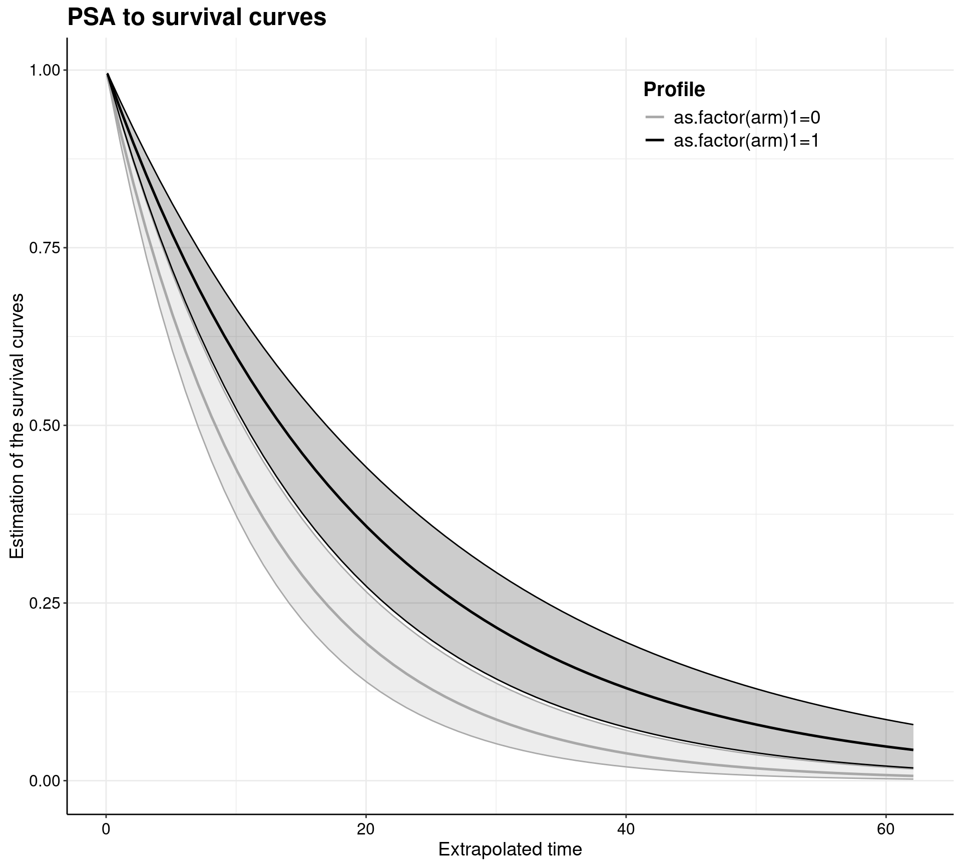
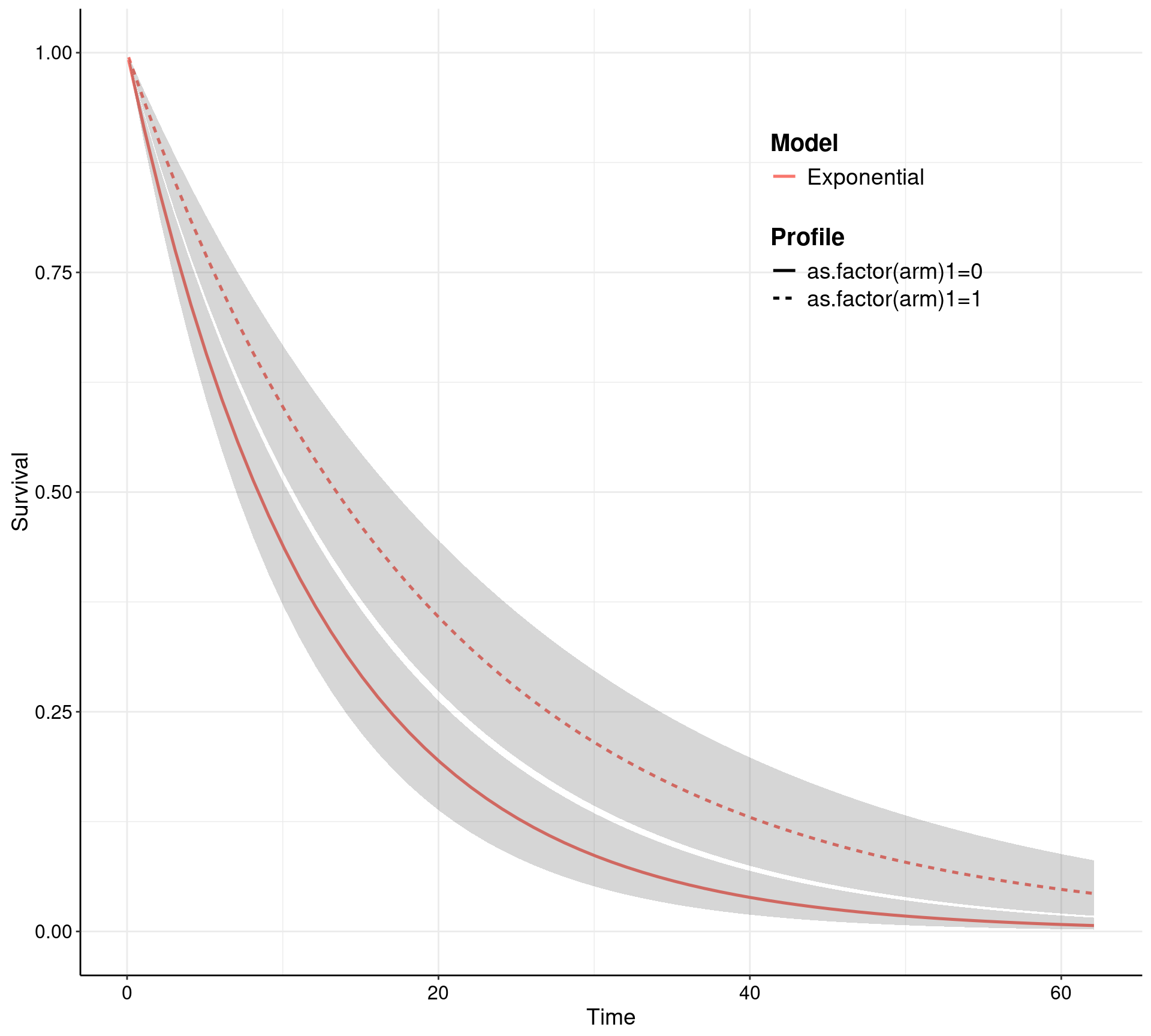
Notice that make.surv (which is called either explicitly in the left-hand panel, or implicitly through the plot method in the right-hand panel) allow for a direct extrapolation of the survival curves — this is one of the key feature of survival modelling in health economics. In this case, the survival curves, together with 95% interval estimates, are shown over a time horizon spanning up to 63, while the observed data are only up to about time = 21.
Of course, our recommendation is to perform the whole of the modelling (that includes the statistical model, the economic model, the PSA and the final decision-making process) in R. This reduces the possibility of errors (for instance through copy and paste across different software) and more importantly takes full advantage of a computing environment that is fit for purpose (as opposed to spreadsheets that are great at doing what they are designed to do, but can be spectacularly bad at tasks they shouldn’t be asked to do!). In addition, performing the complete analysis in R makes it possible to link to other tools (to remain in our own backyard, this, this or this — but many more are available and mentioned here).
But: if the user really has to, survHE allows them to automatically write the simulated values for the survival curves onto an xlsx file.
# Writes the results of the PSA to an Excel file, containing the simulations for the survival curves
write.surv(psa, file = "temp.xlsx")
These can then be post-processed and used to construct the rest of the economic model, for instance in terms of a Markov model — again, if you must this can be done in Excel, but we recommend very strongly against doing so and insted suggest that, once you’ve come this far, you can continue to work in R!
Conclusions
There are many more options and possibilities when working with survHE — and many more are under development. These include using “flexible” methods (e.g. Royston-Parmar Splines or Poly-Weibull distributions) and there are many options for customisation of the results/outputs. These can be explored in the survHE tutorial paper in JSS and, as mentioned above, we welcome additional case-studies or vignettes generated by real experience of the modellers.