Cost-effectiveness acceptability curve plots

BCEA

Bayesian statistics

Health economics

Authors

Gianluca Baio

Nathan Green

Published

September 23, 2020

Introduction

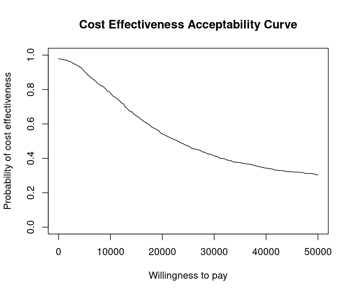
The intention of this vignette is to show how to plot different styles of cost-effectiveness acceptability curves using the BCEA package.

Two interventions only

This is the simplest case, usually an alternative intervention (\(i=1\)) versus status-quo (\(i=0\)).

The plot show the probability that the alternative intervention is cost-effective for each willingness to pay, \(k\),

\[ p(NB_1 \geq NB_0 | k) \mbox{ where } NB_i = ke - c \]

Using the set of \(N\) posterior samples, this is approximated by

\[ \frac{1}{N} \sum_j^N \mathbb{I} (k \Delta e^j - \Delta c^j) \]

R code

To calculate these in BCEA we use the bcea() function.

data("Vaccine")

he <- bcea(eff, cost)
#> No reference selected. Defaulting to first intervention.
# str(he)

ceac.plot(he)

The plot defaults to base R plotting. Type of plot can be set explicitly using the graph argument.

ceac.plot(he, graph = "base")

ceac.plot(he, graph = "ggplot2")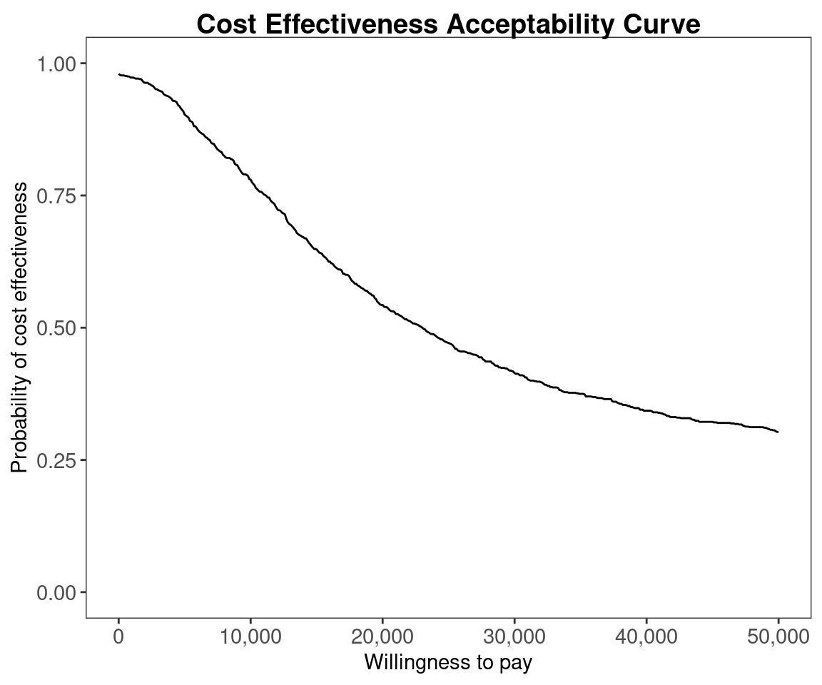

# ceac.plot(he, graph = "plotly")

Other plotting arguments can be specified such as title, line colours and theme.

ceac.plot(he,
          graph = "ggplot2",
          title = "my title",
          line = list(colors = "green"),
          theme = theme_dark())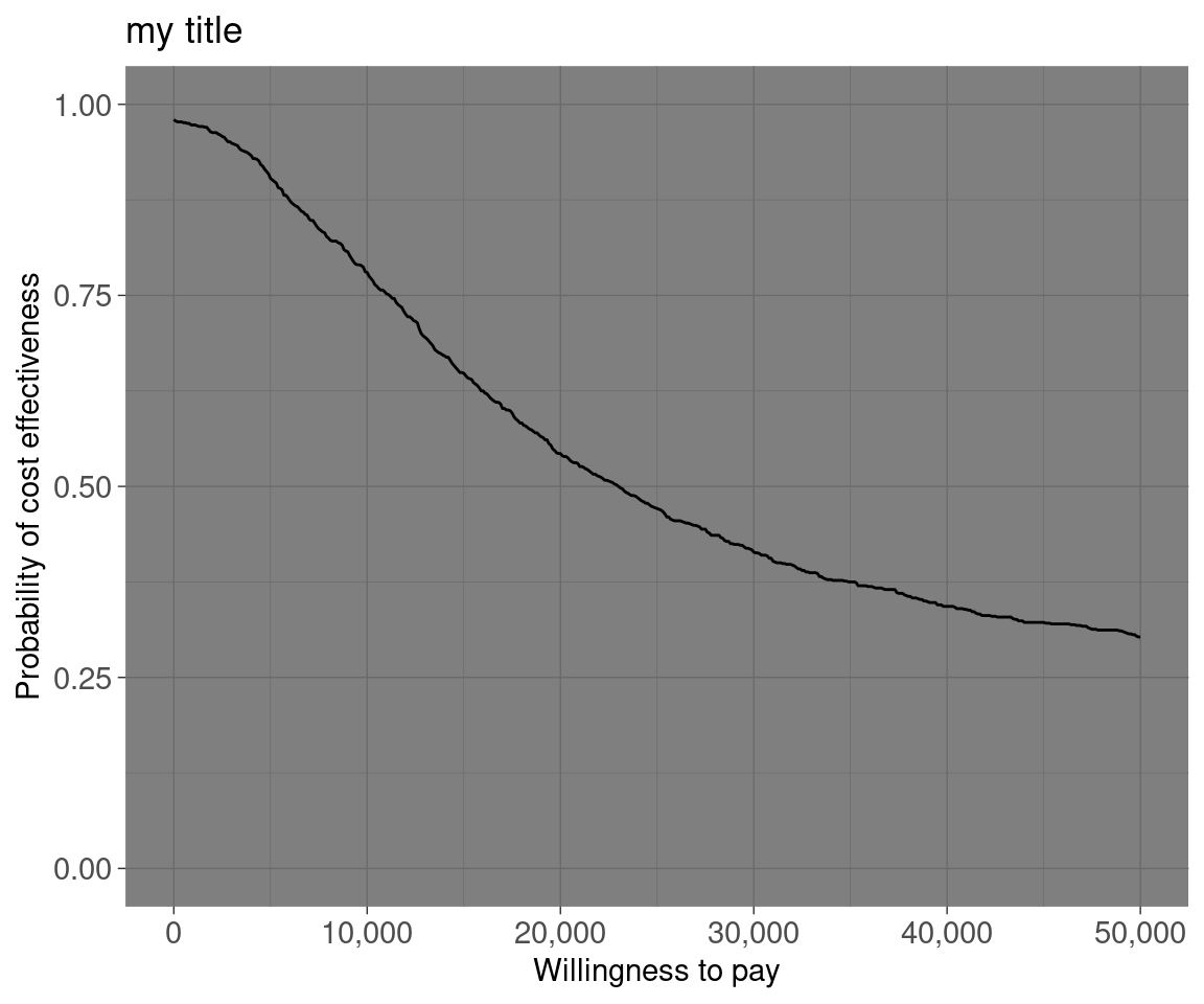

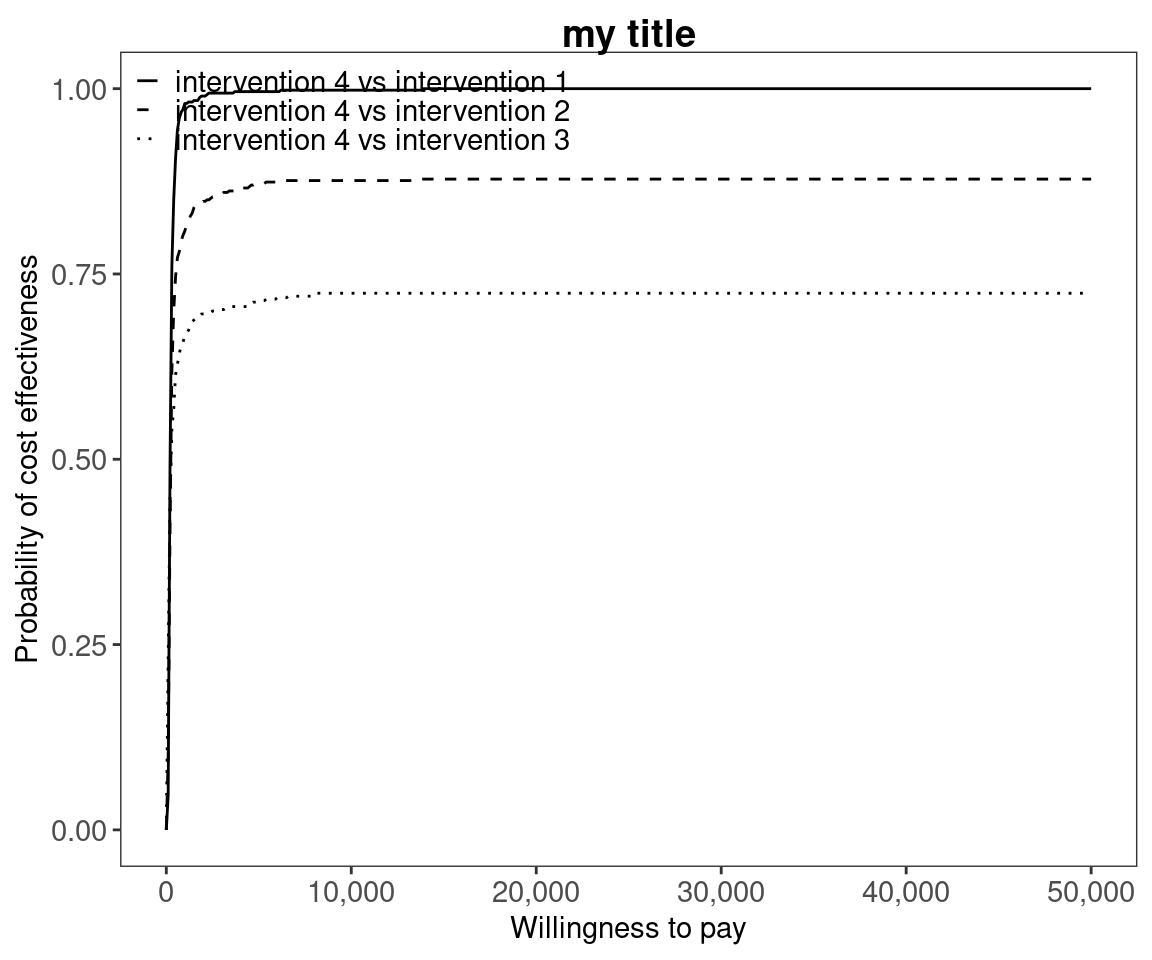
Multiple interventions

This situation is when there are more than two interventions to consider. Incremental values can be obtained either always against a fixed reference intervention, such as status-quo, or for all pair-wise comparisons.

Against a fixed reference intervention

Without loss of generality, if we assume that we are interested in intervention \(i=1\), then we wish to calculate

\[ p(NB_1 \geq NB_s | k) \;\; \exists \; s \in S \]

Using the set of \(N\) posterior samples, this is approximated by

\[ \frac{1}{N} \sum_j^N \mathbb{I} (k \Delta e_{1,s}^j - \Delta c_{1,s}^j) \]

R code

This is the default plot for ceac.plot() so we simply follow the same steps as above with the new data set.

data("Smoking")

he <- bcea(eff, cost, ref = 4)
# str(he)

ceac.plot(he)


ceac.plot(he,
          graph = "base",
          title = "my title",
          line = list(colors = "green"))

ceac.plot(he,
          graph = "ggplot2",
          title = "my title",
          line = list(colors = "green"))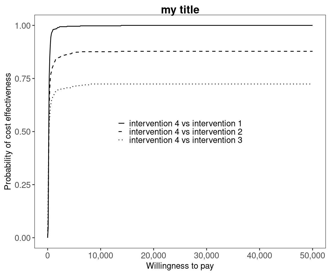

Reposition legend.

ceac.plot(he, pos = FALSE) # bottom right

ceac.plot(he, pos = c(0, 0))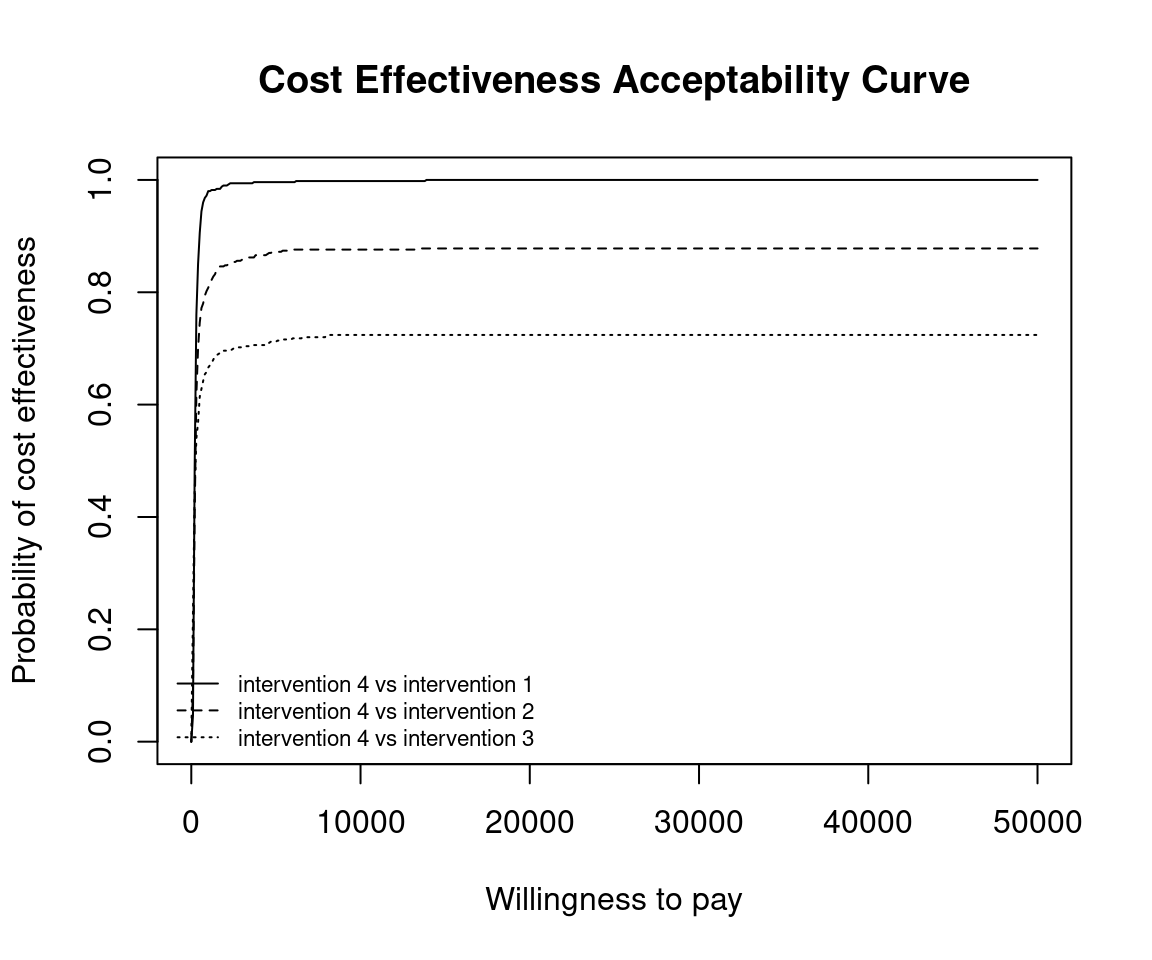

ceac.plot(he, pos = c(0, 1))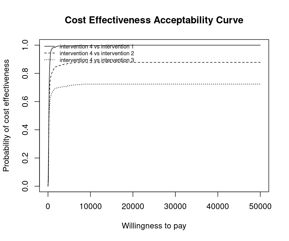

ceac.plot(he, pos = c(1, 0))

ceac.plot(he, pos = c(1, 1))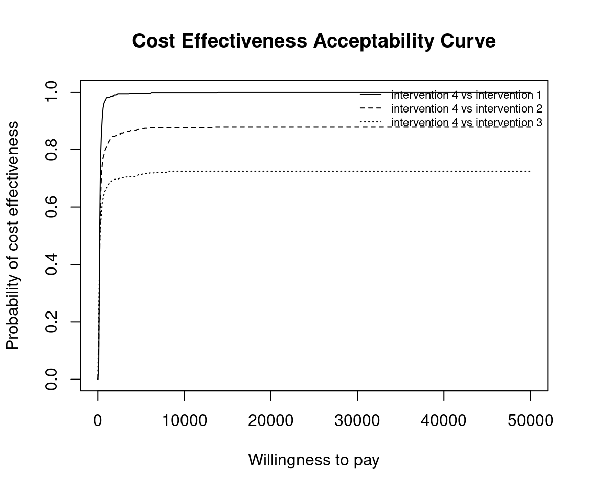

ceac.plot(he, graph = "ggplot2", pos = c(0, 0))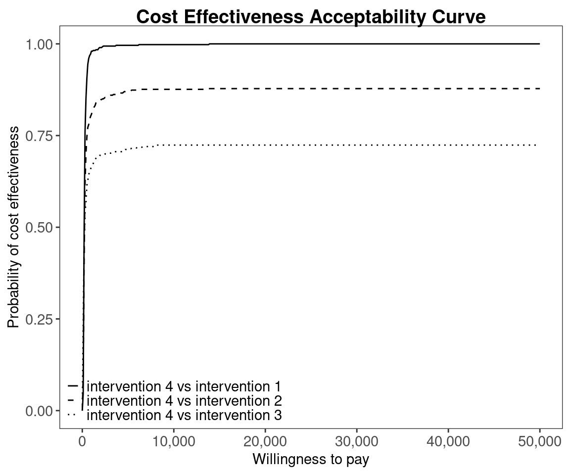

ceac.plot(he, graph = "ggplot2", pos = c(0, 1))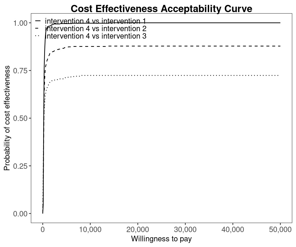

ceac.plot(he, graph = "ggplot2", pos = c(1, 0))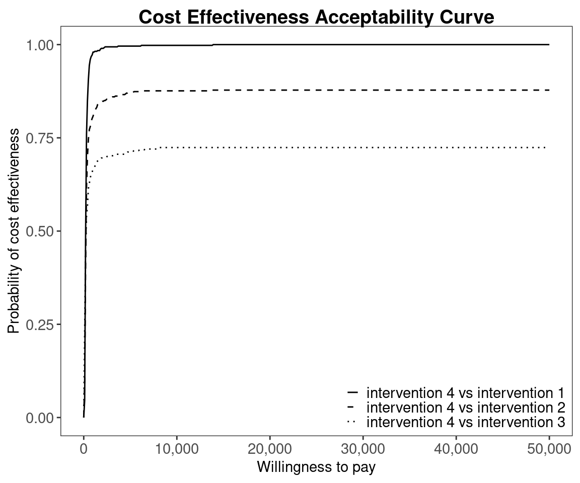

ceac.plot(he, graph = "ggplot2", pos = c(1, 1))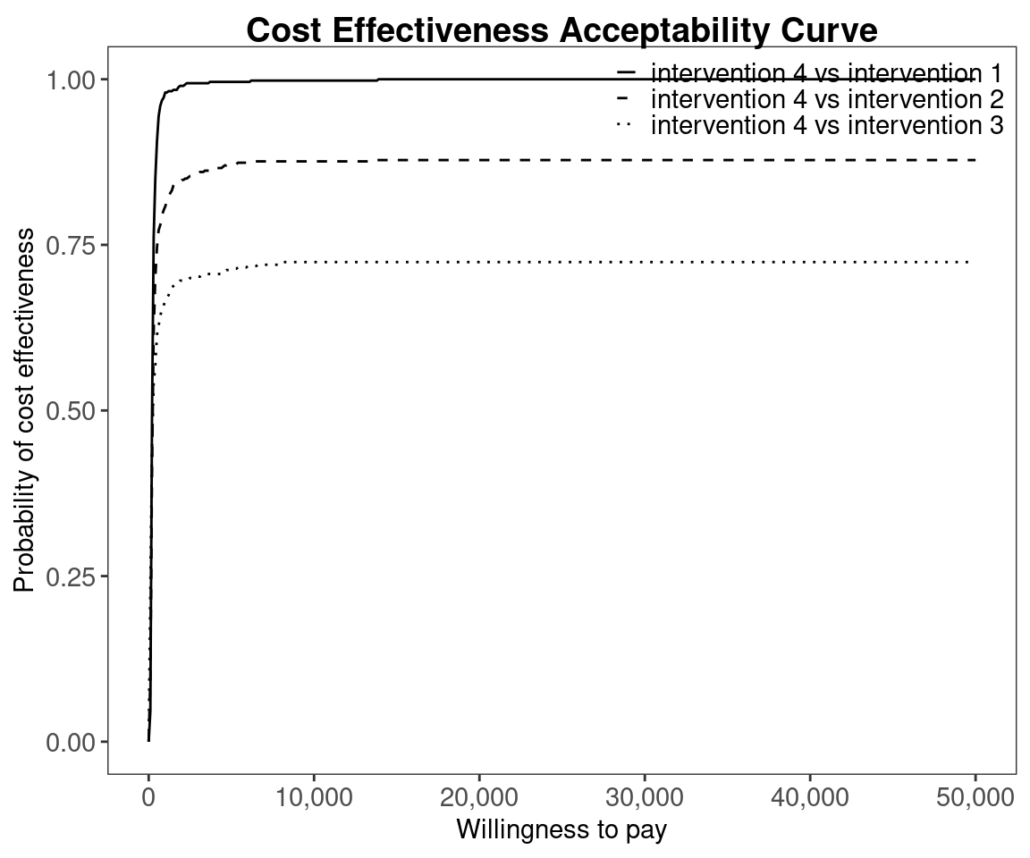

Define colour palette.

mypalette <- RColorBrewer::brewer.pal(3, "Accent")

ceac.plot(he,
          graph = "base",
          title = "my title",
          line = list(colors = mypalette),
          pos = FALSE)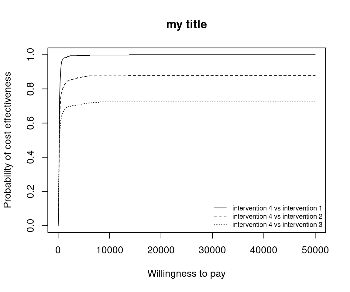


ceac.plot(he,
          graph = "ggplot2",
          title = "my title",
          line = list(colors = mypalette),
          pos = FALSE)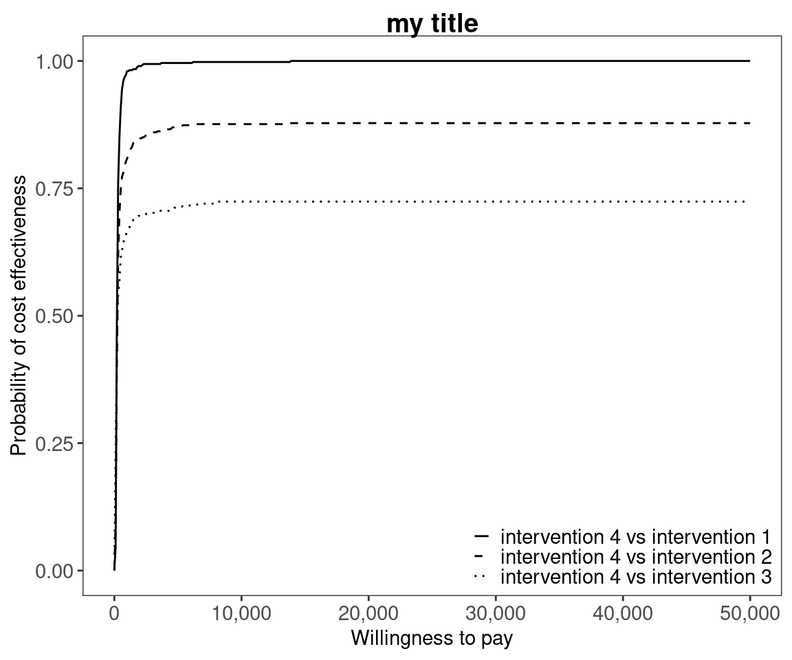

Pair-wise comparisons

Again, without loss of generality, if we assume that we are interested in intervention \(i=1\), the we wish to calculate

\[ p(NB_1 = \max\{NB_i : i \in S\} | k) \]

This can be approximated by the following.

\[ \frac{1}{N} \sum_j^N \prod_{i \in S} \mathbb{I} (k \Delta e_{1,i}^j - \Delta c_{1,i}^j) \]

R code

In BCEA we first we must determine all combinations of paired interventions using the multi.ce() function.

he2 <- multi.ce(he)

We can use the same plotting calls as before i.e. ceac.plot() and BCEA will deal with the pairwise situation appropriately. Note that in this case the probabilities at a given willingness to pay sum to 1.

ceac.plot(he, graph = "base")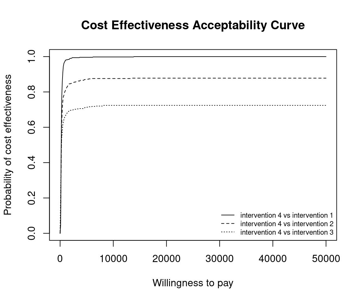


ceac.plot(he,
          graph = "base",
          title = "my title",
          line = list(colors = "green"),
          pos = FALSE)


mypalette <- RColorBrewer::brewer.pal(4, "Dark2")

ceac.plot(he,
          graph = "base",
          title = "my title",
          line = list(colors = mypalette),
          pos = c(0,1))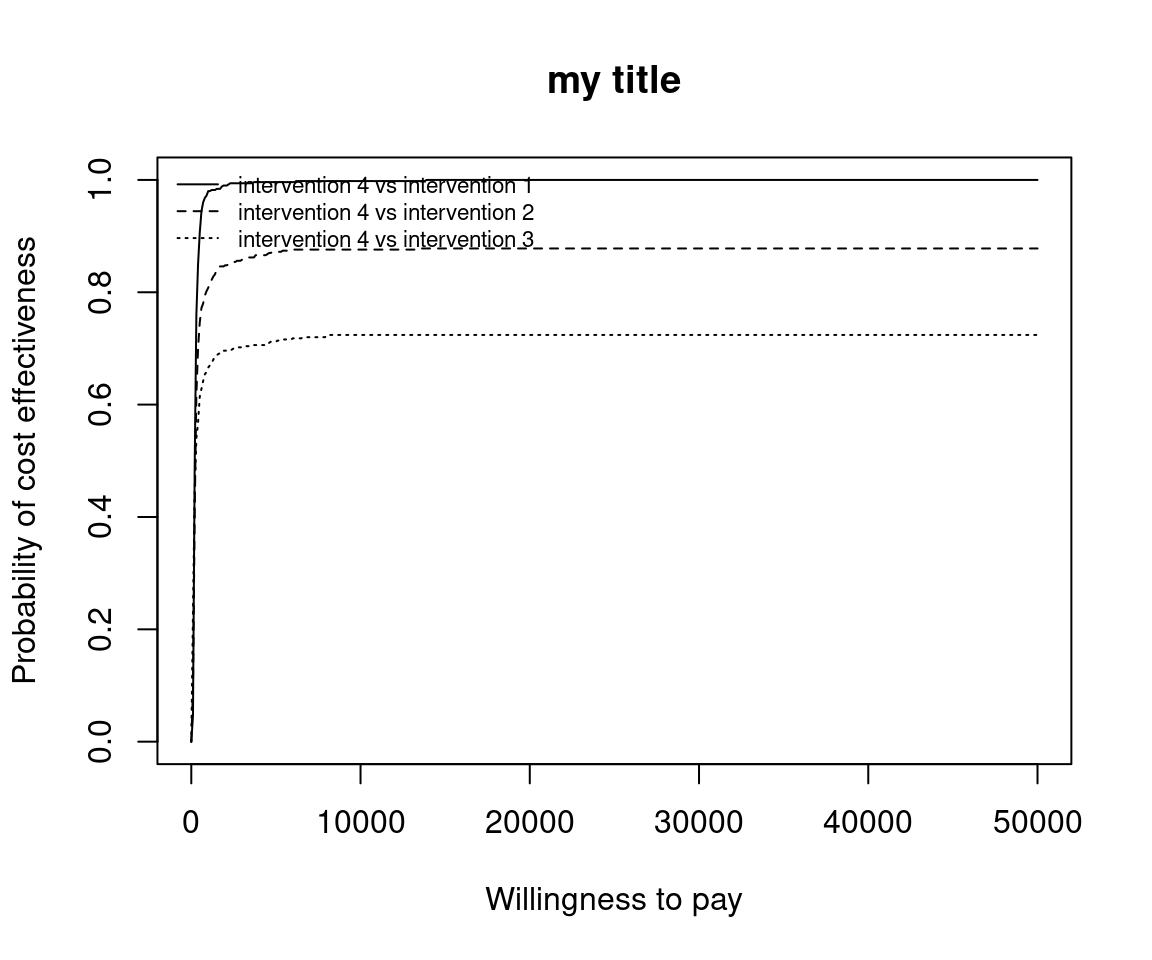

ceac.plot(he,
          graph = "ggplot2",
          title = "my title",
          line = list(colors = mypalette),
          pos = c(0,1))