Data Analysis Using Regression and Multilevel/Hierarchical Models
Multiparameter evidence synthesis
Introduction
Unusual for a policy question to be informed by a single study
Must use all available and relevant evidence
Multiparameter evidence synthesis
Learning about more than one quantity from combination of direct and indirect evidence
Example: Network Meta Analysis (NMA)
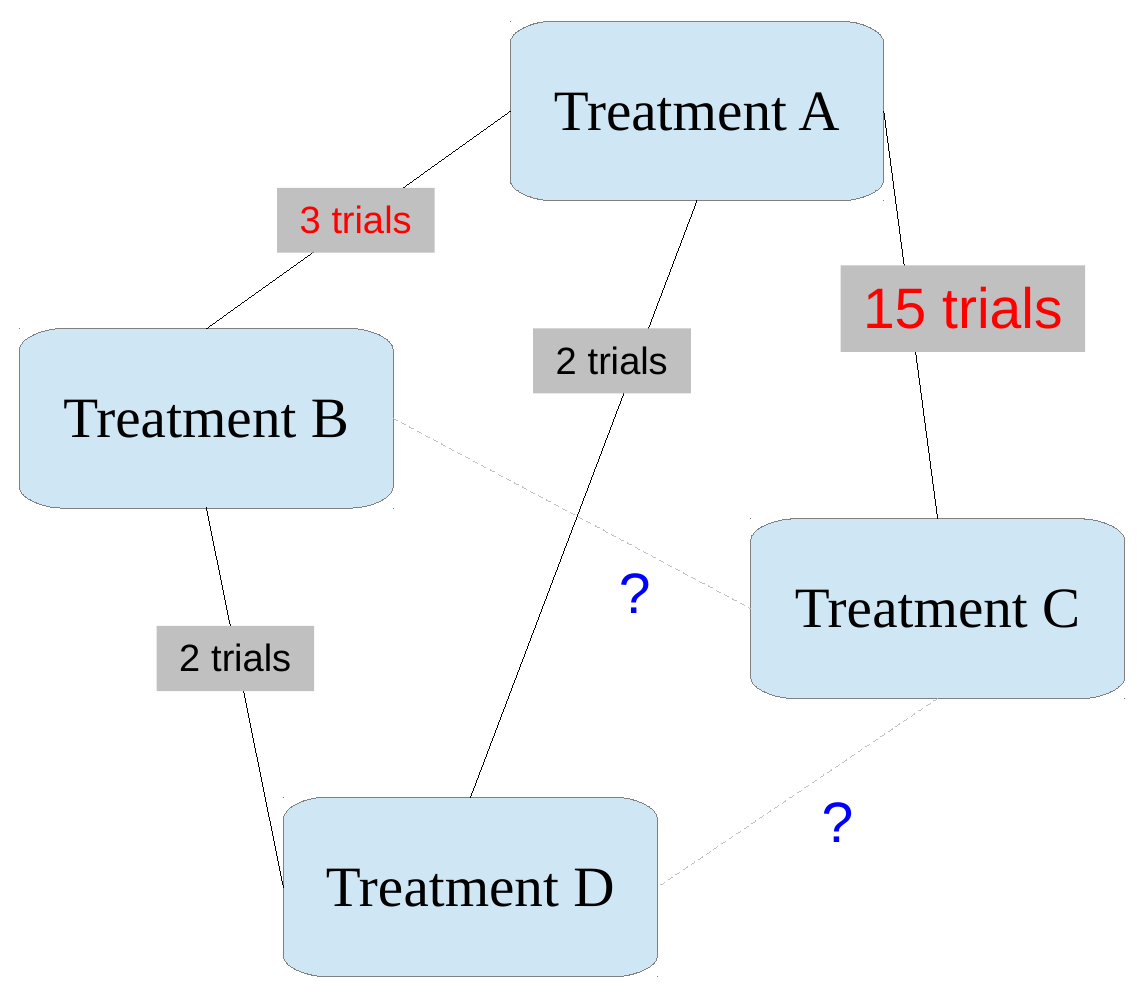
Network Meta Analysis
Simplest example
New treatment C: been trialled against old treatment B, but not to A
For health economic evaluation need to compare A/B/C together
Learn about C/A effect from C/B and B/A trial data
Also called “mixed treatment comparisons”
Since can also “mix” direct and indirect data on same comparison…
Common in UK health technology assessment, but require some statistical skills!
Smoking cessation trial
Data
Comparison
A: No intervention
B: Self-help
C: Individual counselling
D: Group counselling
AB
79 / 702
77 / 694
18 / 671
21 / 535
8 / 116
19 / 149
AC
75 / 731
363 / 714
2 / 106
9 / 205
58 / 549
237 / 1561
0 / 33
9 / 48
3 / 100
31 / 98
1 / 31
26 / 95
6 / 39
17 / 77
64 / 642
107 / 761
5 / 62
8 / 90
20 / 234
34 / 237
95 / 1107
143 / 1031
15 / 187
36 / 504
78 / 584
73 / 675
69 / 1177
54 / 888
ACD
9 / 140
23 / 140
10 / 138
AD
0 / 20
9 / 20
BC
20 / 49
16 / 43
BCD
11 / 78
12 / 85
29 / 170
BD
7 / 66
32 / 127
CD
12 / 76
20 / 74
9 / 55
3 / 26
Outcome
Successfully quit smoking by 6-12 months
Number of success / number of participants
Set up
24 trials in total
Network of comparisons involving 4 interventions
Not all interventions tested against all others!
Objective
Estimate the overall effectiveness of the interventions
Potentially add cost-effectiveness analysis
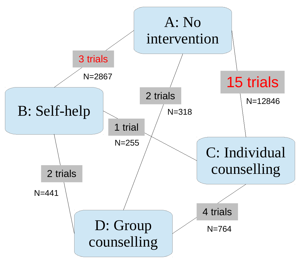
Smoking cessation trial
Network of comparisons
All comparisons have at least one trial with direct data
We wish to enhance direct with indirect evidence
e.g. A-D comparison (only 2 direct trials) improved by including A-C, C-D trials (15 + 4)
In general…
Network of comparisons
In other applications, might want to learn about comparisons with no direct trial evidence
e.g. how much better than current treatment C is new treatment D?
“Fixed effects” NMA
Log odds of response in each arm modelled as effect of study\(\class{red}{s}\) plus effect of treatment\(\class{red}{t}\)\((s = 1, \ldots , NS\), different values of \(t\) in each \(s)\)
Study effects\(\mu_s\): log odds in baseline group of study \(s\), considered independent between studies
Treatment effects
\(\delta_{st}\): compared to study\(\class{red}{s}\) baseline \(t_{s_{s0}}\) \(d_t\): compared to overall baseline treatment \(t=1\) (e.g. placebo) \(\Rightarrow d_1 :=0\) - This essentially means that the effect of treatment \(t=1\) versus the effect of the baseline treatment (again \(t=1\)) is… nothing \((=0)\)!
“Fixed” effects: \(d_t\) are identical in each study \(s\)
\(\log \OR\)s \(d_B\), \(d_C\), \(d_D\) (compared to “baseline” treatment A) are directly identifiable from A-B, A-C, A-D trials
But: can deduce indirect comparisons from these basic parameters (with assumptions…)
\(\log\OR\) of C compared to B is \(d_C-d_B\)
\(\log\OR\) of D compared to B is \(d_D-d_B\)
\(\log\OR\) of D compared to D is \(d_D-d_C\)
NB This assumes consistency between indirect and (potential) direct evidence!
Consider \(t=B\)
By definition: \(\logit(p_{st}) = \log\left(\frac{p_{st}}{1-p_{st}}\right) =\log\) odds of the event (quit smoking), if you are in group B
Similarly, \(\logit(p_{sA}) = \log\left(\frac{p_{sA}}{1-p_{sA}}\right) =\log\) odds of the event (quit smoking), if you are in group A \((\Rightarrow t=1)\)
     [,1] [,2] [,3] [,4]
[1,]   79   77   NA   NA
[2,]   18   21   NA   NA
# ...and the last 4 rows of the data for the number of quitters in each armtail(smoke.list$r,4)
      [,1] [,2] [,3] [,4]
[21,]   NA   11   12   29
[22,]   NA    7   NA   32
[23,]   NA   NA   12   20
[24,]   NA   NA    9    3
# In study 1, treatments 3 (=C) and 4 (=D) are not present so the data show 'NA'# Similarly, in study 21, treatment 1 (=A) was not involved, so there's a 'NA'
# Similarly, shows the first 2 rows...head(smoke.list$n,2)
     [,1] [,2] [,3] [,4]
[1,]  702  694   NA   NA
[2,]  671  535   NA   NA
# ...and the last 4 rows of the data for the total sample size in each armtail(smoke.list$n,4)
      [,1] [,2] [,3] [,4]
[21,]   NA   78   85  170
[22,]   NA   66   NA  127
[23,]   NA   NA   76   74
[24,]   NA   NA   55   26
# Here shows the first 2 and last 4 rows of the matrix indicating the treatment included in the comparisonhead(smoke.list$t,2)
     t1 t2 t3
[1,]  1  2 NA
[2,]  1  2 NA
tail(smoke.list$t,4)
      t1 t2 t3
[21,]  2  3  4
[22,]  2  4 NA
[23,]  3  4 NA
[24,]  3  4 NA
# So in study number 1, the comparison is between intervention 1 (=A) and intervention 2 (=B)# while in study number 21, the comparison is among interventions 2 (=B), 3 (=C) and 4(=D)
# What are the treatment involved in study 21?smoke.list$t[21,]
t1 t2 t3
 2  3  4
# What is the number of quitters in study 21 and in the second treatment arm of that study?smoke.list$r[21,smoke.list$t[21,2]]
[1] 12
# What is the sample size in study 21 and in the second treatment arm of that study?smoke.list$n[21,smoke.list$t[21,2]]
[1] 85
Coding NMA in BUGS/JAGS
Just write out the equations-ish… 😉
NB: t[s,a] indicates the treatment associated with study s and its arm a
Vague priors for effects / baseline are typically OK
But not when the number of comparisons is very small!
for(s in1:NS) {for (a in1:na[s]) { r[s,t[s,a]] ~dbin(p[s,t[s,a]], n[s,t[s,a]])logit(p[s,t[s,a]]) <- mu[s] + delta[s,t[s,a]] }# delta are effects compared to arm 1 of each study s delta[s,t[s,1]] <-0for (a in2:na[s]) { delta[s,t[s,a]] <- d[t[s,a]] - d[t[s,1]] }}for (i in1:NS){# vague prior for baseline log-odds mu[i] ~dnorm(0,0.0001) }# effect compared to treatment 1 (e.g. placebo)d[1] <-0# vague priorfor (i in2:NT) { d[i] ~dnorm(0, 0.0001) }
Presenting treatment effects
For each treatment \(2, \ldots, NT\) compared to treatment 1 (the reference/baseline: eg “no intervention”/“status quo”, or placebo), can back-transform the \(\log\OR\)s
for (t in2:NT) { or[t] <-exp(d[t]) # odds ratios}
Then can compute the odds ratio for every other treatment pair c, k – even if no direct comparison exist
\(\OR_{ck} = \OR_{c1} / \OR_{k1}\)
for (c in1:(NT-1)) {for (k in (c+1):NT) { or[c,k] <-exp(d[c] - d[k]) or[k,c] <-1/or[c,k] }}
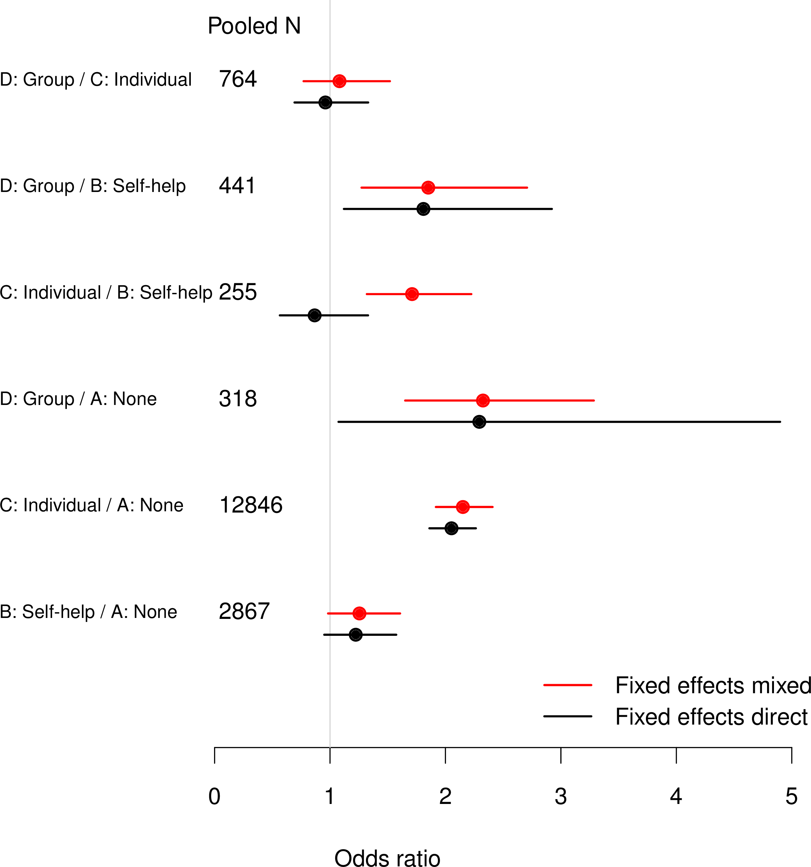
Results
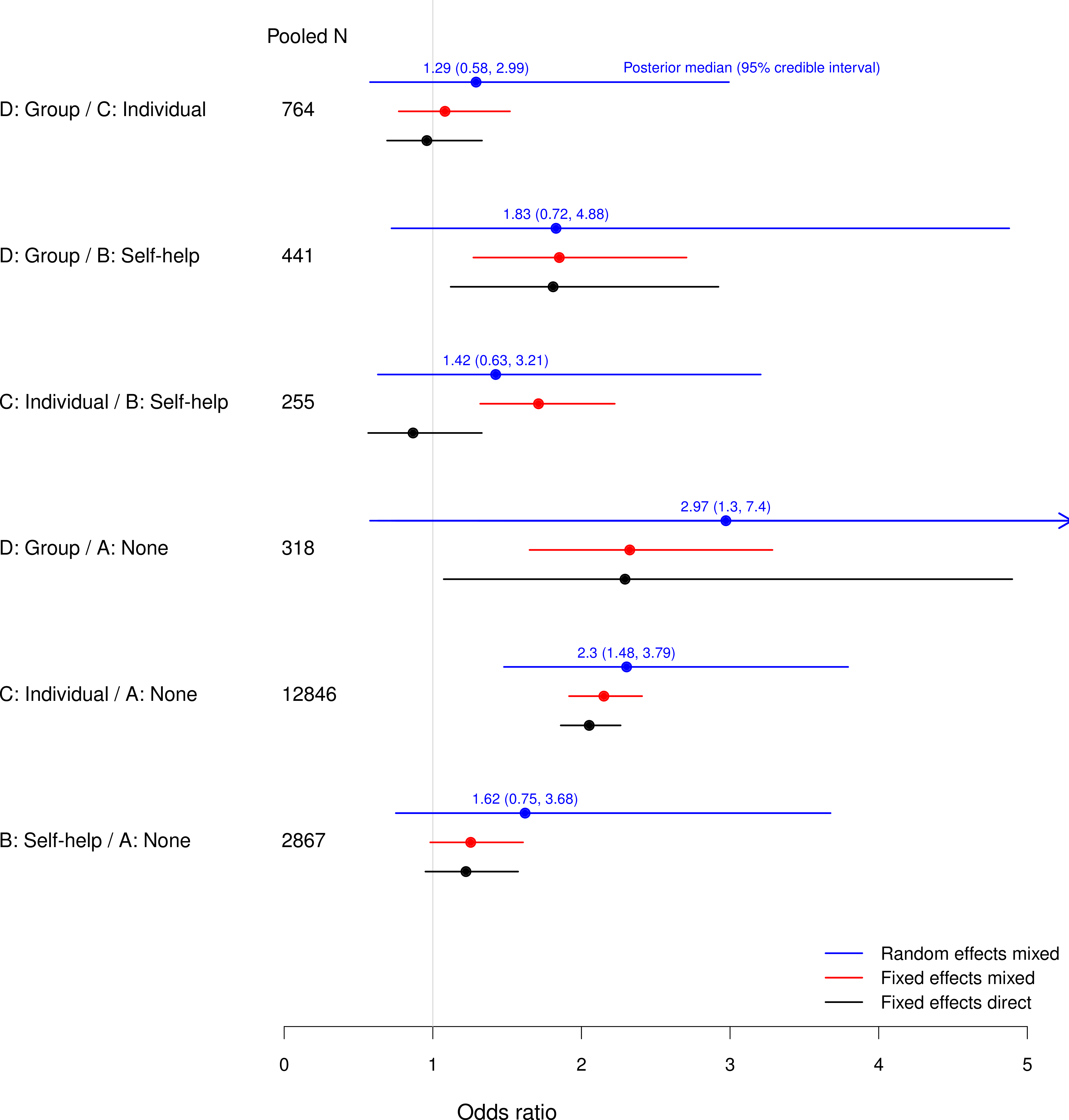
Comparing direct and mixed evidence
Direct-only odds ratios (CIs) from classical analysis of pooled individual data
Precision of D/A estimate improved by indirect C/A and C/D data
Strong direct data for other comparisons, so not improved much by indirect evidence
C/B estimate from one direct study \(\Rightarrow\) pulled towards much bigger indirect C/A and B/A data
evidence of heterogeneity…
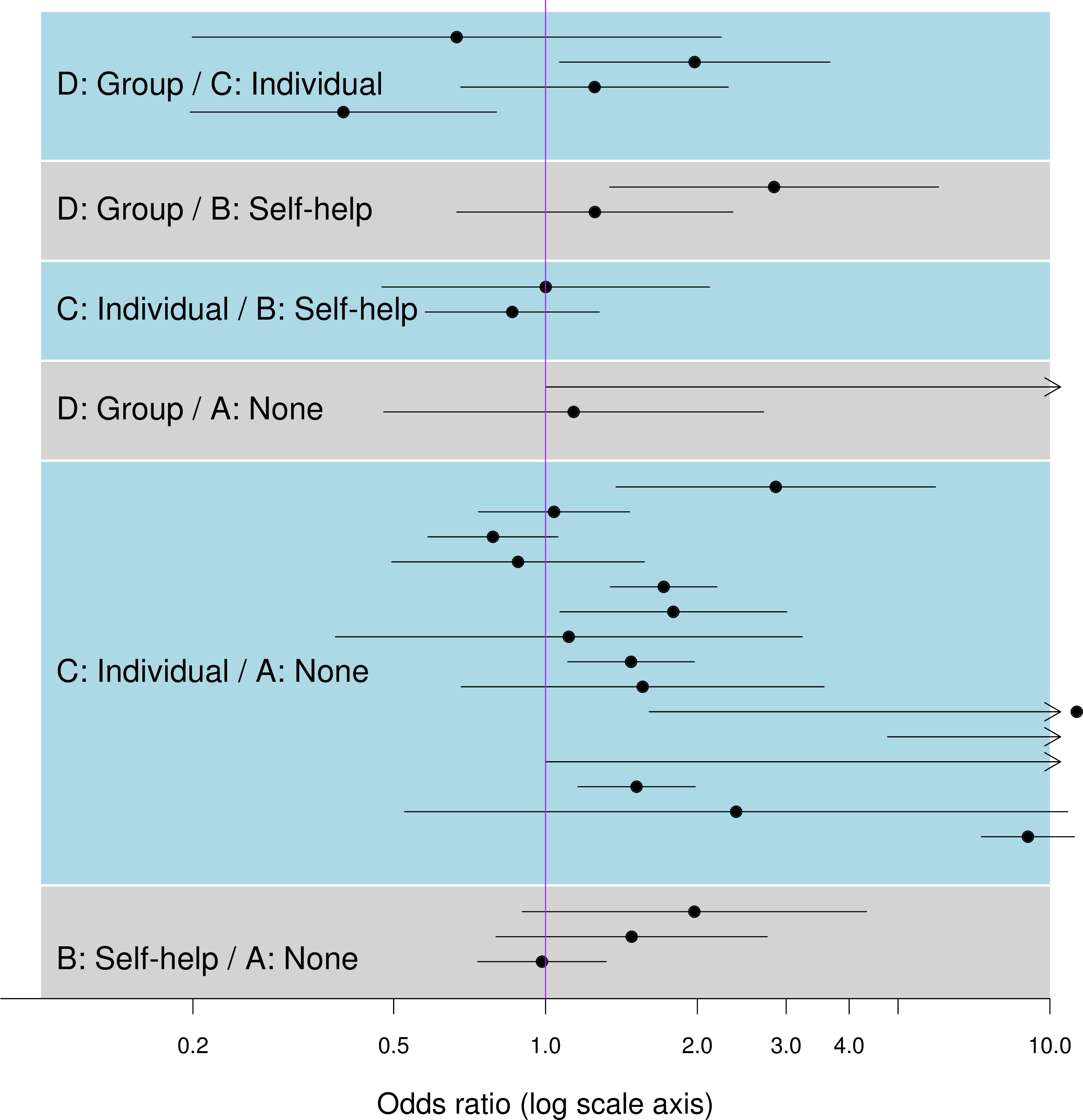
Results
Heterogeneity between individual studies
Classical odds ratio (CIs) for all individual trials, sorted by pairwise comparison
Heterogeneity between ORs within most comparisons
Consider “random” effects models…
Random effects NMA
Replace fixed effects\(\delta_{st}\) of treatment \(t\) in study \(s\)
with a .red[random effect] varying between studies \(s\) with a Normal distribution with mean defined by the fixed effect \[\begin{align}
& \class{myblue}{r_{st}} \class{myblue}{\sim} \class{myblue}{\dbin(p_{st},n_{st})} \\
& \class{myblue}{\logit(p_{st})} \class{myblue}{=}\class{myblue}{\mu_s + \delta_{st}} \\
& \class{myblue}{\delta_{st}\sim\dnorm(\mu_{st}^\delta, \sigma^2_{st})} \\
& \class{myblue}{\mu_{st}^\delta}\class{myblue}{=} \class{myblue}{d_t - d_{t_{s0}}}
\end{align}\]
still with \(\delta_{st}=0\) for \(t=\) baseline arm of \(s\)
Coding this in BUGS/JAGS
Equations translate relatively straight to BUGS model, again:
for (a in2:na[s]) { delta[s,t[s,a]] <- d[t[s,a]] - d[t[s,1]]}
is replaced by:
for (a in2:na[s]) { delta[s,t[s,a]] ~dnorm(md[s,t[s,a]], taud[s,t[s,a]]) md[s,t[s,a]] <- d[t[s,a]] - d[t[s,1]] taud[s,t[s,a]] <- tau}d[1] <-0# Priors on the mean same as fixed effectsfor (i in2:NT) { d[i] ~dnorm(0, 0.0001) }
But: a couple of complicating features…
Constraints on random effects variances
In a NMA, we have
\(NT\) different treatments
\((NT - 1)\) different pooled effects, relative to treatment 1 (the baseline / reference) Only 1 effect in standard meta-analysis
\((NT-1)\) different random effects distributions to estimate?
Not feasible unless many studies of every single treatment
\(\Rightarrow\)identifiability constraints needed
Assume same random effects variance for each treatment comparison
Prior for\(\class{red}{\sigma^2}\): Uniform from 0 to a large upper limit (eg 10 if on the log scale) is often used, especially to align with standard meta-analysis
But: Beware of sensitivity to this — particularly if only few studies are considered…
Results
Random effects models
Wider CIs after accounting for heterogeneity
C/B: compromise between direct and indirect evidence
D/A: smallest trials, still a lot of uncertainty
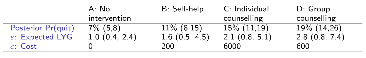
Use in cost-effectiveness analysis
Example
External data on Expected Life-Years Gained if quit smoking:
around 15 years (sd \(\approx\) 4): model as \(L\sim \dnorm(\style{font-family:inherit;}{\text{mean}} =15,\style{font-family:inherit;}{\text{sd}}=4)\)
and code this as L ~ dnorm(15, 0.0625) in BUGS
Model \(L\) by Prob(quit) to get E[LYG] under each intervention
and compare to cost of each intervention:
Further issues…
Different type of outcomes
Binary data (Binomial models, as here)
Counts of events/person-years at risk (Poisson models)
Mean + sd of continuous outcomes (Normal models) … in each arm of the study
Individual patient data alongside data aggregated by arms
Meta-regression: explain heterogeneity between studies using study-level characteristics as covariates
Detecting / handling conflicts between direct / indirect evidence