2. Bayesian computation

Gianluca Baio

Department of Statistical Science   |   University College London

g.baio@ucl.ac.uk

https://gianluca.statistica.it

https://egon.stats.ucl.ac.uk/research/statistics-health-economics

https://github.com/giabaio   https://github.com/StatisticsHealthEconomics  

@gianlubaio@mas.to     @gianlubaio    

Bayesian modelling for economic evaluation of healthcare interventions

València International Bayesian Analysis Summer School, 7th edition, University of Valencia

10 - 11 July 2024

Check out our departmental podcast “Random Talks” on Soundcloud!

Follow our departmental social media accounts + magazine “Sample Space”

Bayesian computation

• Forward sampling (Monte Carlo)
  • Express current knowledge as parameters with distributions
  • Simulate parameters, make predictions from models based on the parameters
  • Like a spreadsheet with randomness on cells. Familiar in health economics as “probabilistic sensitivity analysis”
  • Doesn’t really need specialised software

• Learning from data (model fitting)
  • Compute posterior distributions combining prior and data, through Bayes’ theorem
  • Simpler models — do not require specialised software
    • “Vague” priors
    • “Conjugate” analysis
  • Realistic models — MCMC
    • eg: Gibbs sampling

Bayesian computation

Generally speaking, the computational effort depends in large part on the definition of the prior…

1. Uniform prior \[ p(\theta\mid y) = \frac{p(\theta)p(y\mid \theta)}{p(y)} \propto \frac{c\mathcal{L}(\theta\mid y)}{c\int\mathcal{L}(\theta\mid y)d\theta} \propto \frac{\mathcal{L}(\theta\mid y)}{\int \mathcal{L}(\theta\mid y)d\theta} \]

2. Conjugate prior \[p(\theta) \in f(\theta; \bm{a}) \quad\Rightarrow\quad p(\theta\mid y) \propto p(\theta)\mathcal{L}(\theta\mid y) \in f(\theta; \bm{a^*})\]

3. All other (real-life) cases…
   • Can write algorithms to simulate from an unknown target (posterior) distribution
   • General-purpose software to deal with all cases…
   • BUGS/JAGS/Stan/Nimble
   • INLA

General software for Bayesian computation

Different versions of BUGS

• WinBUGS 1.4.3
  • Original release 1997 — runs only on Windows
  • Stable but no longer developed (latest release: August 2007)
  • Freely available from http://www.mrc-bsu.cam.ac.uk/bugs
• OpenBUGS http://www.openbugs.net
  • Open-source offshoot, also runs on Linux and MacOS
  • Works just as well, stable

“Rivals”/alternatives

• JAGS http://mcmc-jags.sourceforge.net
  • Language essentially identical, Work just as well, stable
  • Runs natively on Mac/Unix/Windows
• Stan http://mc-stan.org/
  • Probabilistic language — slightly different than BUGS/JAGS
  • Based on different algorithm — can be more efficient in some cases

Interfaces exist to run these from other software, eg (R2OpenBUGS, R2jags, rstan) Excel, S-Plus, SAS, Matlab, Stata, …

BUGS/JAGS

• Language for specifying Bayesian models as a network of known and unknown quantities

Example: linear regression

\[\begin{eqnarray*} y_i & \sim & \dnorm(\mu_i,\sigma) \qquad \mbox{for } i=1,\ldots,N \\ \mu_i & = & \alpha+\beta x_i \\ \tau & \sim & \dgamma(0.01,0.01)\\ \sigma & = & \tau^{-0.5} \\ \alpha & \sim & \dnorm(0,0.01) \\ \beta & \sim & \dnorm(0,0.01) \end{eqnarray*}\]

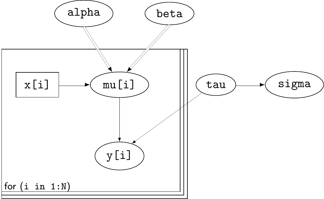
model {
  for (i in 1:N) {
     y[i] ~ dnorm(mu[i], tau)
     mu[i] <- alpha + beta*x[i]
  }
  tau ~ dgamma(0.1,0.1)
  sigma <- pow(tau,-0.5)
  alpha ~ dnorm(0,0.01)
  beta ~ dnorm(0,0.01)
}

• BUGS/JAGS have a built-in parser, which inspects the set of declarations and translates them into a DAG
• Exploits as much as possible the underlying conditional independence relationships to speed up computation

Example — drug

• Consider a drug to be given for relief of chronic pain
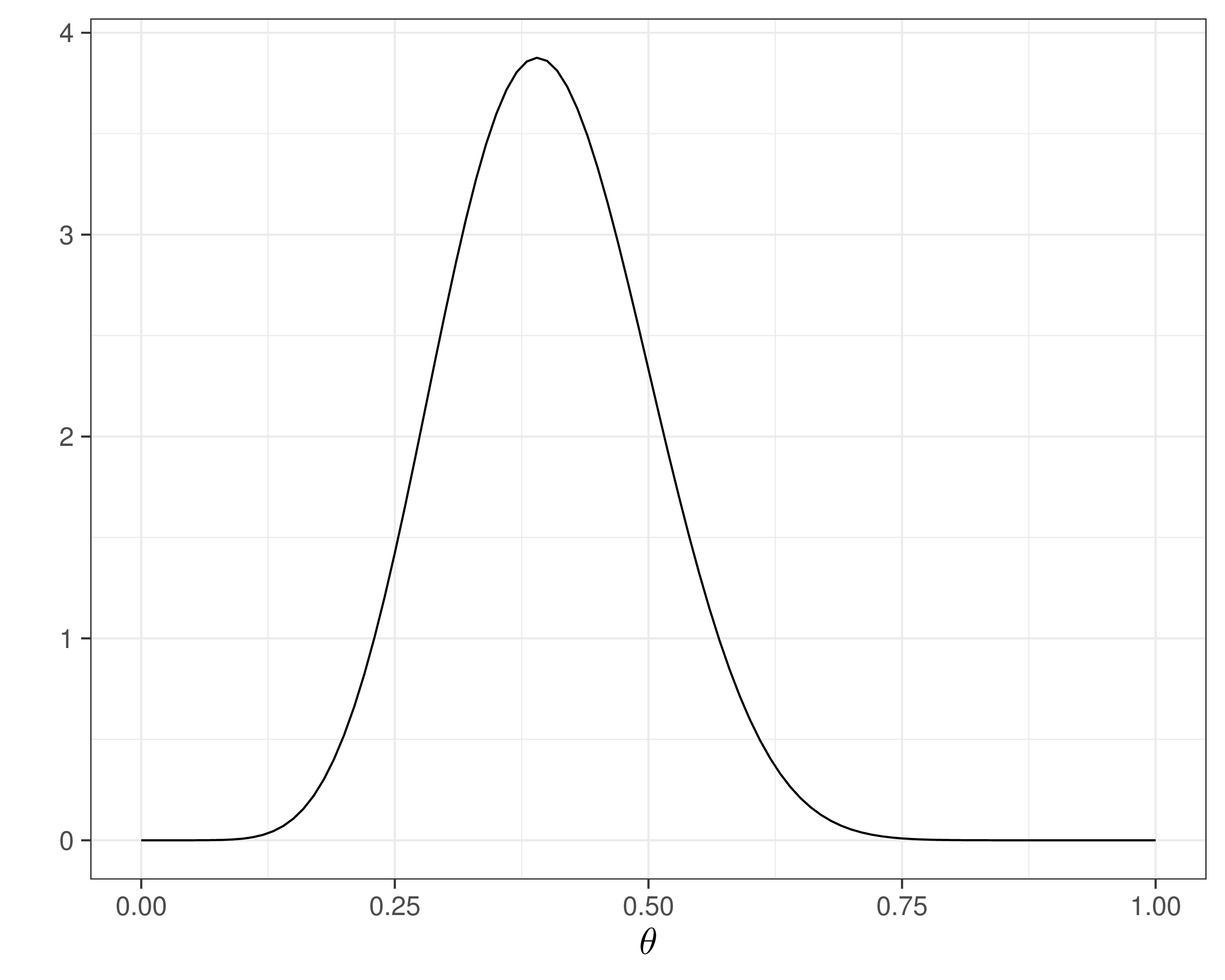
• Experience with similar compounds has suggested that annual response rates between 0.2 and 0.6 could be feasible
• Interpret this as a distribution with mean = 0.4 and standard deviation = 0.1
• Can encode these into a Beta(9.2, 13.8) prior

Example — drug

• Suppose we can actually run a small pilot study, in which we observe \(y=15\) in \(n=20\) individuals to whom we give the drug and who are relieved from the back pain
• Update uncertainty over \(\theta\) = probability of “success” for the drug
• Predict number of successes in the next \(m=40\) patients

• Can model using

\[\begin{eqnarray*} y & \sim & \dbin(\theta, n) \\ \theta & \sim & \dbeta(a,b) \\ y_{pred} & \sim & \dbin(\theta, m) \end{eqnarray*}\]

NB: \(p(y_{pred}\mid y)\) is the predictive distribution

• Mixes up (revised/posterior) uncertainty in \(\theta\) and sampling variability (Binomial model)

Running JAGS from R

Map the “pen-and-paper” model into JAGS code

• Can code up the model in a .txt. file

  model {
    theta ~ dbeta(a,b)
    y ~ dbin(theta,n)
    y.pred ~ dbin(theta,m)
  }

• … OR write directly in R as a function

  model.code=function(){
    theta ~ dbeta(a,b)
    y ~ dbin(theta,n)
    y.pred ~ dbin(theta,m)
  }

In R, provide the observed data

data=list(
  a=9.2, b=13.8,
  y=15,
  n=20,
  m=40
)

Use JAGS to obtain the posterior and the predictive distributions

# Loads the relevant R package to interface with JAGS
library(R2jags)

# Runs the model
m=jags(
  data=data,
  parameters.to.save=c("y.pred","theta"),
  inits=NULL,
  model.file=model.code,
  n.chains=2,
  n.iter=6000,
  n.burnin=1000,
  n.thin=1
)

Running JAGS from R

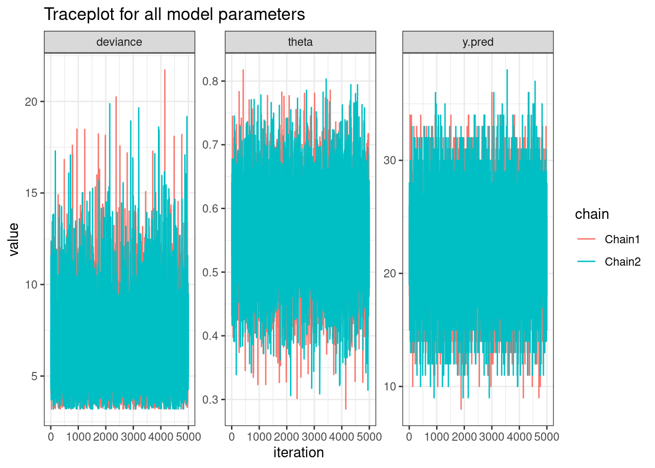
• The object m contains the MCMC output

# Shows the names of the elements inside the object 'm'
m |> names()

[1] "model"              "BUGSoutput"         "parameters.to.save"
[4] "model.file"         "n.iter"             "DIC"               

• Can explore further and see where various bits are… (but don’t really need to do so…)

# 'BUGSoutput' is the main element
m$BUGSoutput |> names()

 [1] "n.chains"        "n.iter"          "n.burnin"        "n.thin"         
 [5] "n.keep"          "n.sims"          "sims.array"      "sims.list"      
 [9] "sims.matrix"     "summary"         "mean"            "sd"             
[13] "median"          "root.short"      "long.short"      "dimension.short"
[17] "indexes.short"   "last.values"     "program"         "model.file"     
[21] "isDIC"           "DICbyR"          "pV"              "DIC"            
[25] "time2run"       

• Can summarise results directly

print(m,digits=3,intervals=c(.025,.975))

Inference for Bugs model at "/tmp/RtmpGy2l2J/model22c593971f56c.txt", 
 2 chains, each with 6000 iterations (first 1000 discarded)
 n.sims = 10000 iterations saved. Running time = 0.015 secs
         mu.vect sd.vect   2.5%  97.5%  Rhat n.eff
theta      0.563   0.076  0.411  0.708 1.001 10000
y.pred    22.491   4.352 14.000 31.000 1.001 10000
deviance   6.660   2.444  3.372 12.683 1.001 10000

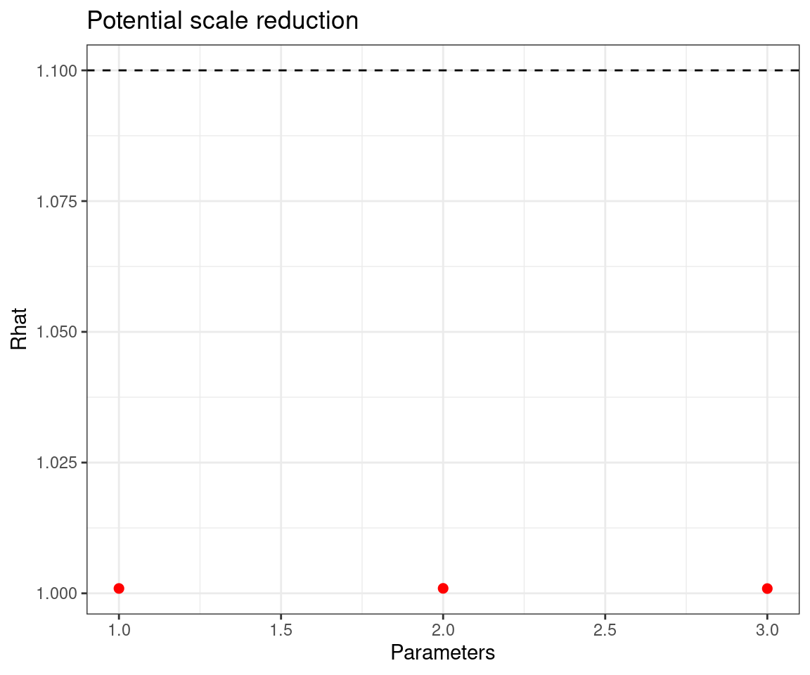
For each parameter, n.eff is a crude measure of effective sample size,
and Rhat is the potential scale reduction factor (at convergence, Rhat=1).

DIC info (using the rule: pV = var(deviance)/2)
pV = 3.0 and DIC = 9.6
DIC is an estimate of expected predictive error (lower deviance is better).

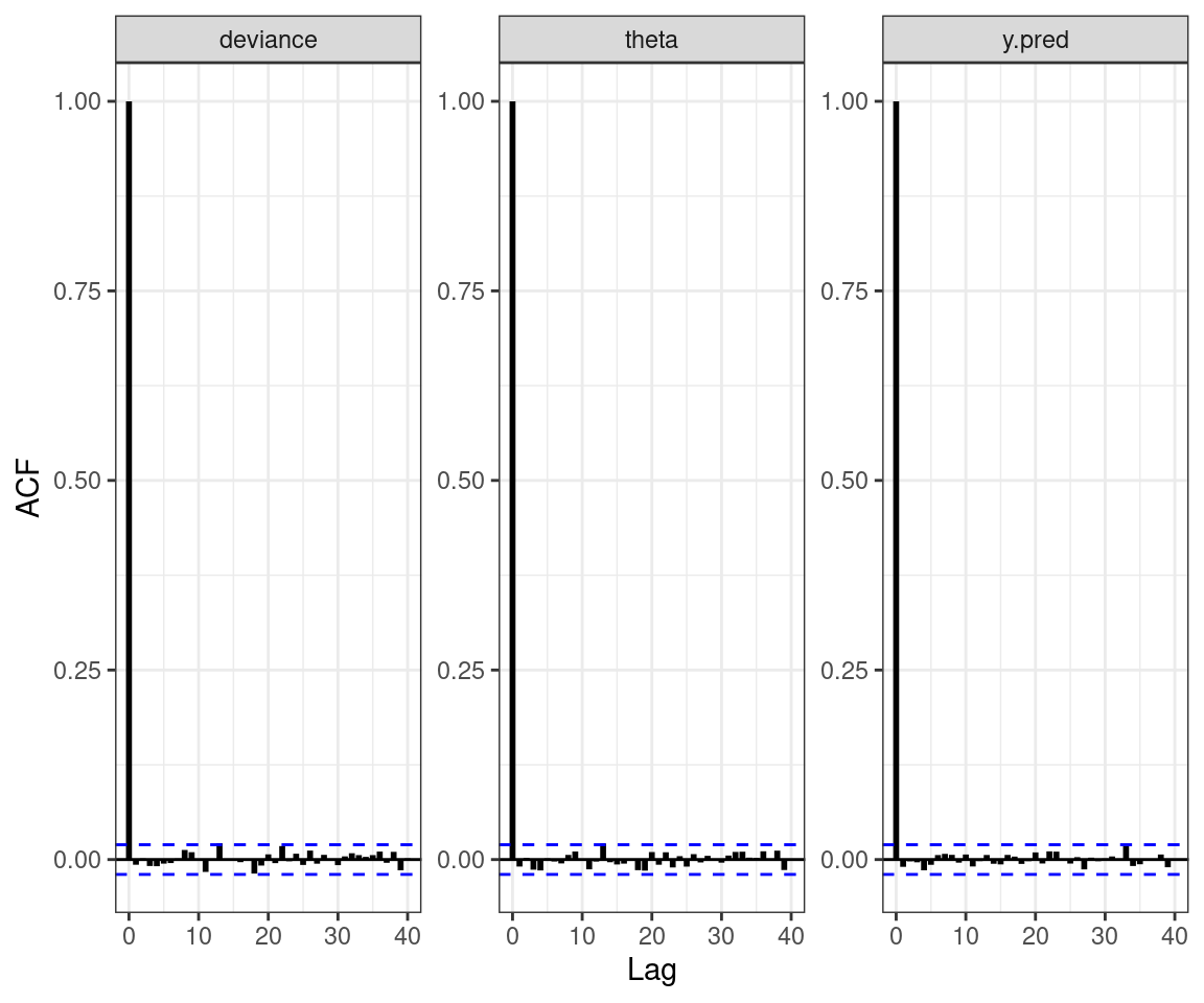
Post-processing the JAGS output

• We can use directly R code to post-process the results
• Or use standardised packages
  • bmhe (for diagnostics & plots)
  • BCEA (for economic evaluation)
  • …

# Installs relevant packages
# Directly from CRAN (main repository)
install.packages("BCEA")
install.packages("R2jags")

# Or from GitHub (more experimental packages)
remotes::install_github("giabaio/bmhe_utils")
remotes::install_github("giabaio/R2jags")

Post-processing the JAGS output

bmhe::traceplot(m)

Post-processing the JAGS output

bmhe::diagplot(m)

Post-processing the JAGS output

bmhe::acfplot(m)