The available data usually look something like this
Demographics
Clinical outcomes
HRQL data
Resource use data
ID
Trt
Sex
Age
\(\ldots\)
\(y_0\)
\(\ldots\)
\(y_J\)
\(u_0\)
\(\ldots\)
\(u_J\)
\(c_0\)
\(\ldots\)
\(c_J\)
1
1
M
23
\(\ldots\)
\(y_{10}\)
\(\ldots\)
\(y_{1J}\)
0.32
\(\ldots\)
0.44
103
\(\ldots\)
80
2
1
M
23
\(\ldots\)
\(y_{20}\)
\(\ldots\)
\(y_{2J}\)
0.12
\(\ldots\)
0.38
1204
\(\ldots\)
877
3
2
F
19
\(\ldots\)
\(y_{30}\)
\(\ldots\)
\(y_{3J}\)
0.49
\(\ldots\)
0.88
16
\(\ldots\)
22
\(\ldots\)
\(\ldots\)
\(\ldots\)
\(\ldots\)
\(\ldots\)
\(\ldots\)
\(\ldots\)
\(\ldots\)
\(\ldots\)
\(\ldots\)
\(\ldots\)
\(\ldots\)
\(\ldots\)
\(\ldots\)
where
\(y_{ij}=\) Survival time, event indicator (eg CVD), number of events, continuous measurement (eg blood pressure), …
\(u_{ij}=\) Utility-based score to value health (eg EQ-5D, SF-36, Hospital & Anxiety Depression Scale), …
\(c_{ij}=\) Use of resources (drugs, hospital, GP appointments), …
Usually aggregate longitudinal measurements into a cross-sectional summary and for each individual consider the pair \({(e_i,c_i)}\). HTA preferably based on utility-based measures of effectiveness
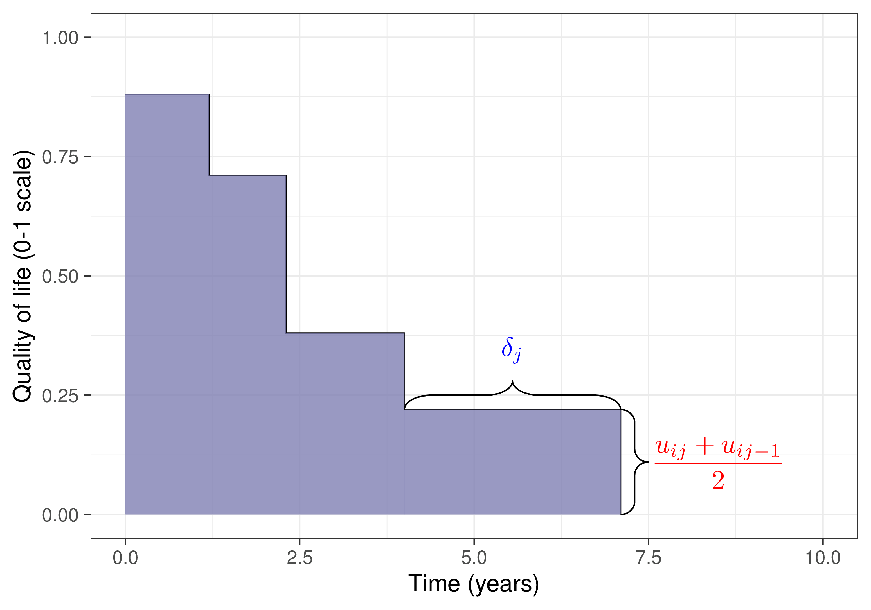
Quality Adjusted Life Years (QALYs) are a measure of disease burden combining
Quantity of life (the amount of time spent in a given health state)
Quality of life (the utility attached to that state)
(Often implicitly) assume normality and linearity and model independently individual QALYs and total costs by controlling for (centered) baseline values, eg \({u^∗_i = (u_i − \bar{u} )}\) and \({c^∗_i = (c_i − \bar{c} )}\)
Estimate population average cost and effectiveness differentials
Under this model specification, these are \(\class{myblue}{\Delta_e=\alpha_{e2}}\) and \(\class{myblue}{\Delta_c=\alpha_{c2}}\)
Quantify impact of uncertainty in model parameters on the decision making process
In a fully frequentist analysis, this is done using resampling methods (eg bootstrap)
Example — 10 Top Tips trial
ID
Trt
Sex
Age
BMI
GP
\(u_0\)
\(u_3\)
\(u_6\)
\(u_{12}\)
\(u_{18}\)
\(u_{24}\)
\(c\)
2
1
F
66
1
21
0.088
0.848
0.689
0.088
0.691
0.587
4230.04
3
1
M
57
1
5
0.796
0.796
0.796
0.620
0.796
1.000
1584.88
4
1
M
49
2
5
0.725
0.727
0.796
0.848
0.796
0.291
331.27
12
1
M
64
2
14
0.850
0.850
1.000
1.000
0.848
0.725
1034.42
13
1
M
66
1
9
0.848
0.848
0.848
1.000
0.848
0.725
1321.30
21
1
M
64
1
3
0.848
1.000
1.000
1.000
0.850
1.000
520.98
Demographics:
BMI = Categorised body mas index
GP = Number of GP visits
HRQL data
QoL measurements at baseline, 3, 6, 12, 18 and 24 months
Costs
Total costs over the course of the study
Computing the QALYs
# Defines a simple function to do the discountingdisc=function(x, year, disc_rate =0.035) { x / ((1+ disc_rate)^(year -1))}# Temporary computation of QoL + QALY with discounting by using long formatdf_qol=ttt |>## select columns of interestselect(id, arm, contains("qol")) |>## convert dataframe from wide to long formatpivot_longer(contains("qol"), names_to ="month", names_prefix ="qol_", names_transform =list(month = as.integer), values_to ="qol" ) |># convert month to follow-up year; set baseline to be in year 1mutate(year =pmax(1, ceiling(month/12))) |>## apply discountingmutate(qol_disc =disc(qol, year)) |># group by individualgroup_by(id) |>mutate(# time duration between measurements delta=month-dplyr::lag(month,default =0),# sum of utilities between two consecutive time pointsdu=qol_disc+dplyr::lag(qol_disc,default =0),# area under the curve (AUC)auc=du*delta/2 ) |># compute the QALYs (in years so divide by 12!), as sum of the AUC # for all time pointssummarise(qaly=sum(auc)/12) |>ungroup()# Merges the overall QALYs to the main datasetttt=ttt |>left_join(df_qol,by=c("id"="id")) |>mutate(Trt=arm+1,arm=factor(arm),arm=case_when(arm=="0"~"Control",TRUE~"Treatment") )ttt
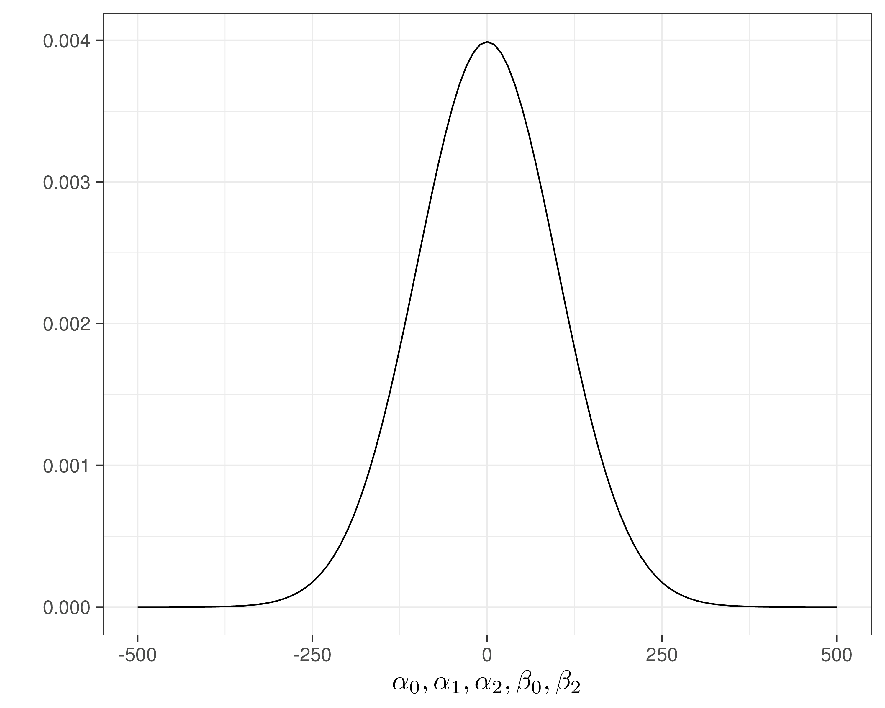
Given the scale of the observed data, unlikely that \(\alpha_0\) and \(\alpha_1\) have such a large range, but given reasonably large sample size, probably won’t matter…
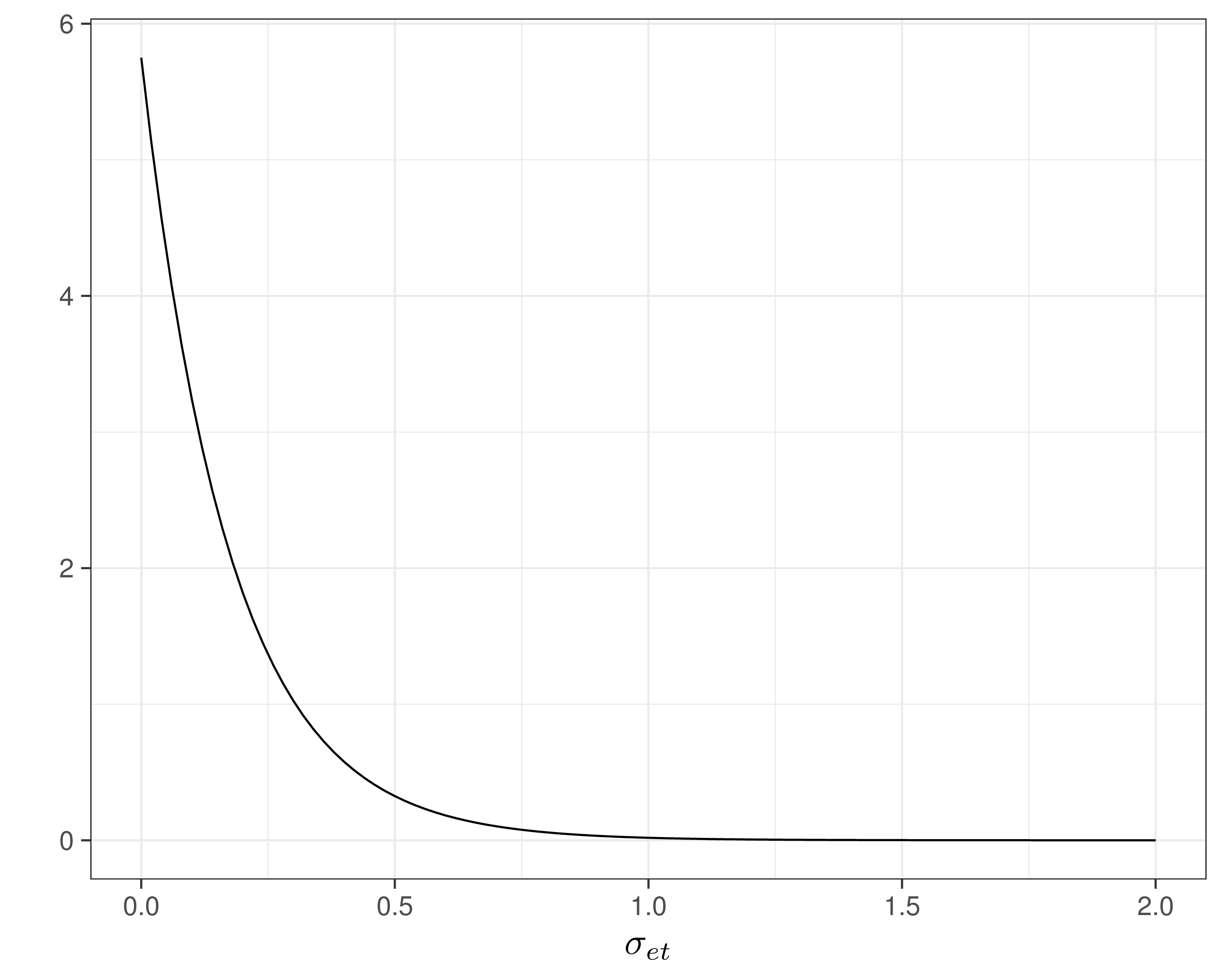
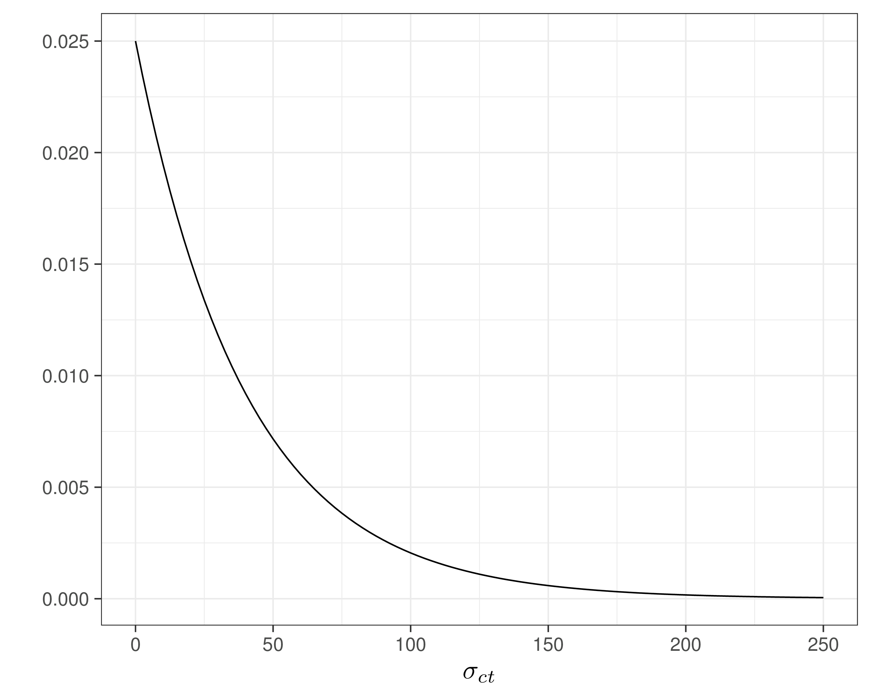
Assume \(\Pr(\sigma_{et}>0.8)\approx 0.01\) and \(=\Pr(\sigma_{ct}>100)\approx 0.1\) — reasonably vague and minimal assumptions
Can use a “Penalty Complexity (PC) prior” to encode these into suitable Exponential distributions with rates \(-\frac{\log(0.01)}{0.8}\approx 5.75\) and \(-\frac{\log(0.1)}{100}\approx 0.025\)
Modelling ILD in HTA
Normal/Normal independent model — model code
# Normal/Normal independent model - JAGS codenn_indep=function(){for (i in1:N) {# Model for the effects e[i] ~dnorm(phi.e[i], tau.e[Trt[i]]) phi.e[i] <- alpha0 + alpha1*(Trt[i]-1) + alpha2*u0star[i]# Model for the costs c[i] ~dnorm(phi.c[i], tau.c[Trt[i]]) phi.c[i] <- beta0 + beta2*(Trt[i]-1) }# Rescales the main economic parametersfor (t in1:2) { mu.e[t] <- alpha0 + alpha1*(t-1) mu.c[t] <- beta0 + beta2*(t-1) }# Minimally informative priors on the regression coefficients alpha0 ~dnorm(0,0.0001) alpha1 ~dnorm(0,0.0001) alpha2 ~dnorm(0,0.0001) beta0 ~dnorm(0,0.0001) beta2 ~dnorm(0,0.0001)for (t in1:2) {# PC-prior on the sd with Pr(sigma_e>0.8) \approx 0.01 sigma.e[t] ~dexp(5.75) tau.e[t] <-pow(sigma.e[t],-2)# PC-prior on the sd with Pr(sigma_c>100) \approx 0.1 sigma.c[t] ~dexp(0.025) tau.c[t] <-pow(sigma.c[t],-2) }}
NB: JAGS (and BUGS…) index the Normal distribution with mean and precision = \(1/\sigma^2\)!
Modelling ILD in HTA
Normal/Normal independent model — running JAGS
# Defines the data listdata=list(e=e,c=c,Trt=Trt,u0star=u0star,N=N)# Initialises the object 'model' as a list to store all the resultsmodel=list()# Runs JAGS in the backgroundlibrary(R2jags)# Stores the BUGS output as an element named 'nn_indep' in the object 'model'model$nn_indep=jags(data=data,parameters.to.save=c("mu.e","mu.c","alpha0","alpha1","alpha2","beta0","beta2","sigma.e","sigma.c" ),inits=NULL,n.chains=2,n.iter=5000,n.burnin=3000,n.thin=1,DIC=TRUE,# This specifies the model code as the function 'nn_indep'model.file=nn_indep)# Shows the summary statistics from the posterior distributions. print(model$nn_indep,digits=3,interval=c(0.025,0.5,0.975))
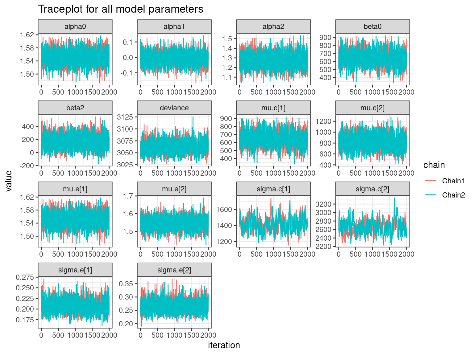
Inference for Bugs model at "/tmp/RtmpMZhrVk/model302f36a5c55d4.txt",
2 chains, each with 5000 iterations (first 3000 discarded)
n.sims = 4000 iterations saved. Running time = 1.296 secs
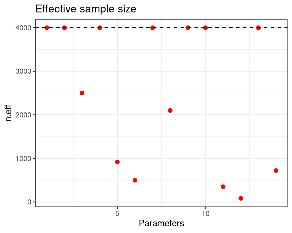
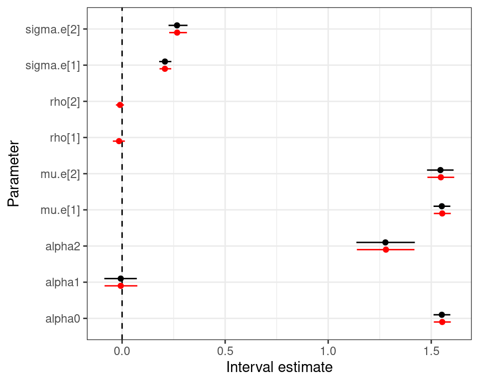
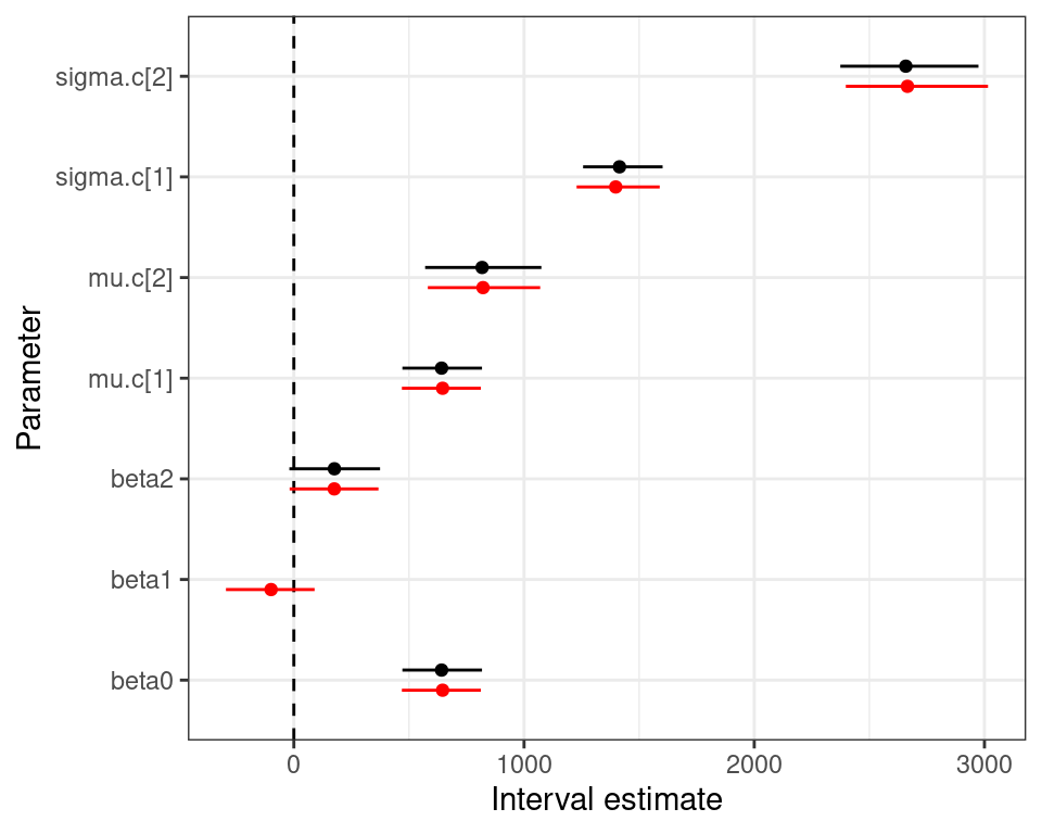
mu.vect sd.vect 2.5% 50% 97.5% Rhat n.eff
alpha0 1.551 0.021 1.511 1.551 1.593 1.001 4000
alpha1 -0.007 0.039 -0.086 -0.007 0.071 1.001 4000
alpha2 1.278 0.072 1.137 1.278 1.421 1.001 2500
beta0 641.695 87.515 471.352 642.276 817.309 1.001 4000
beta2 176.070 99.501 -19.609 175.316 374.427 1.002 920
mu.c[1] 641.695 87.515 471.352 642.276 817.309 1.001 4000
mu.c[2] 817.764 128.646 570.271 818.755 1075.193 1.001 2100
mu.e[1] 1.551 0.021 1.511 1.551 1.593 1.001 4000
mu.e[2] 1.545 0.033 1.480 1.545 1.608 1.001 4000
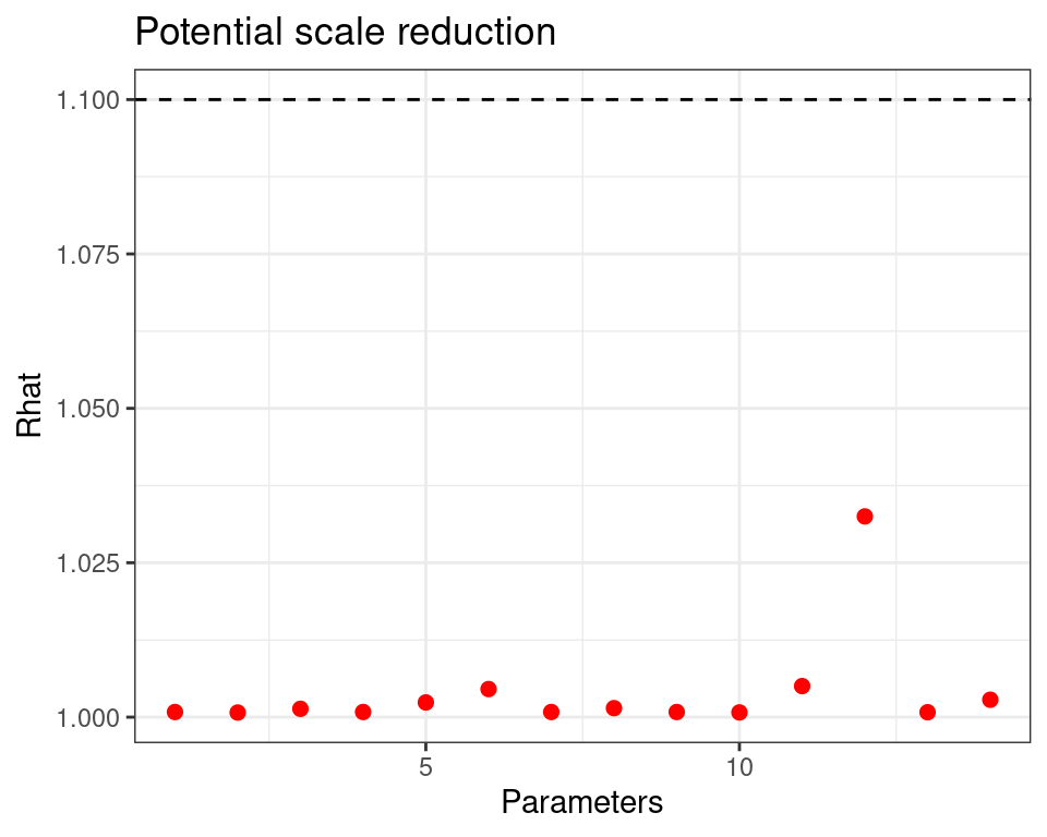
sigma.c[1] 1414.597 89.208 1256.438 1411.066 1601.913 1.005 350
sigma.c[2] 2658.376 154.480 2373.838 2653.705 2973.944 1.033 84
sigma.e[1] 0.208 0.015 0.180 0.207 0.239 1.001 4000
sigma.e[2] 0.267 0.024 0.225 0.265 0.317 1.003 720
deviance 3063.112 12.397 3039.937 3062.619 3088.360 1.005 500
For each parameter, n.eff is a crude measure of effective sample size,
and Rhat is the potential scale reduction factor (at convergence, Rhat=1).
DIC info (using the rule: pV = var(deviance)/2)
pV = 76.7 and DIC = 3139.8
DIC is an estimate of expected predictive error (lower deviance is better).
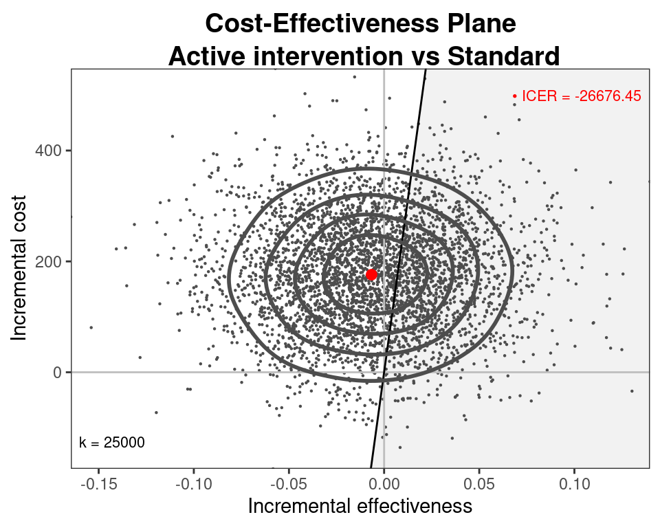
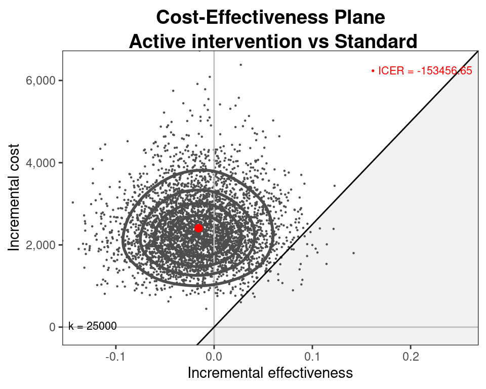
Strong positive correlation – effective treatments are innovative and result from intensive and lengthy research \(\Rightarrow\) are associated with higher unit costs
Negative correlation - more effective treatments may reduce total care pathway costs e.g. by reducing hospitalisations, side effects, etc.
Because of the way in which standard models are set up, bootstrapping generally only approximates the underlying level of correlation – (MCMC does a better job!)
Joint/marginal normality not realistic (Mainly ILD)
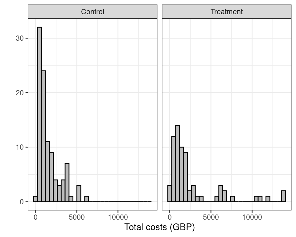
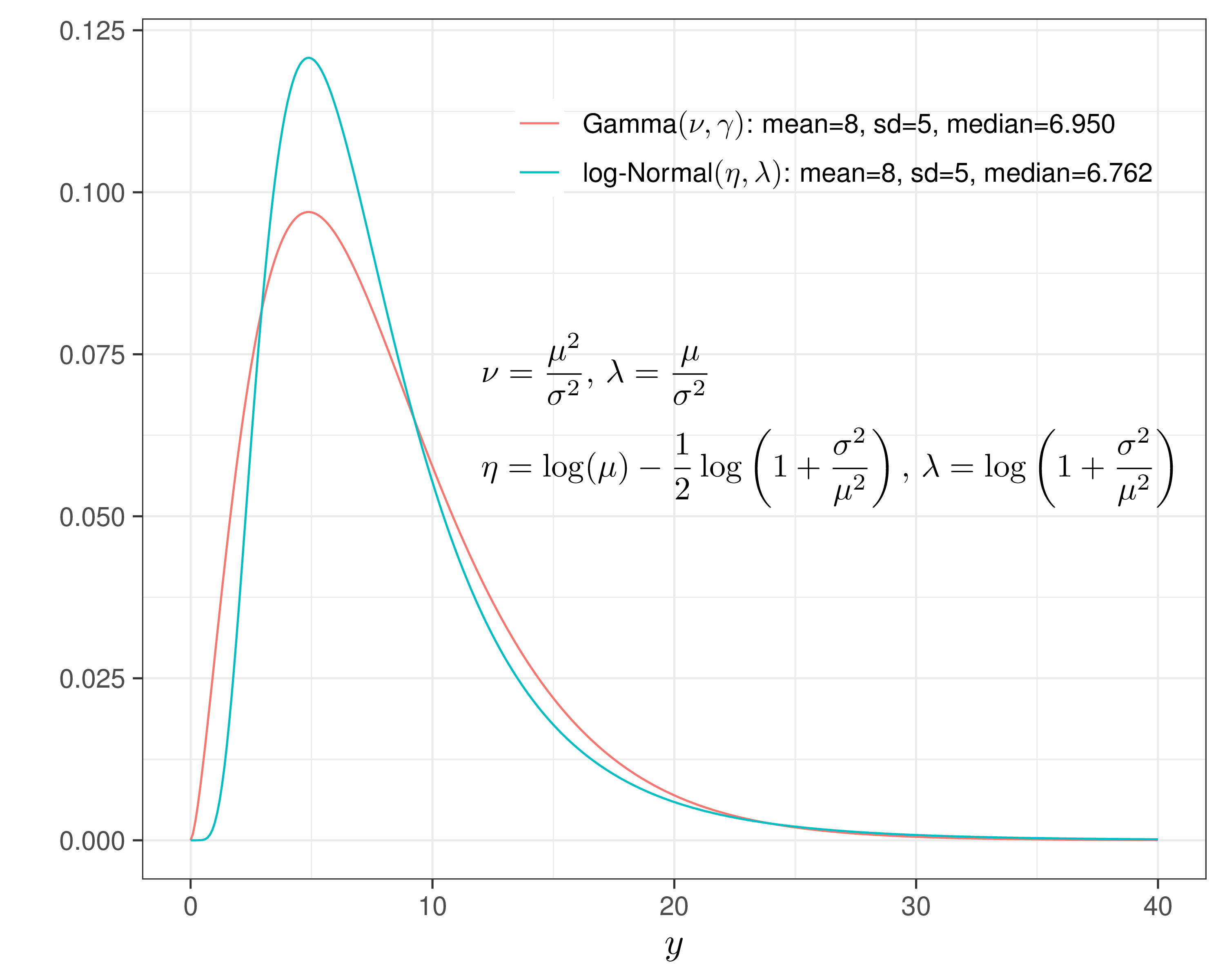
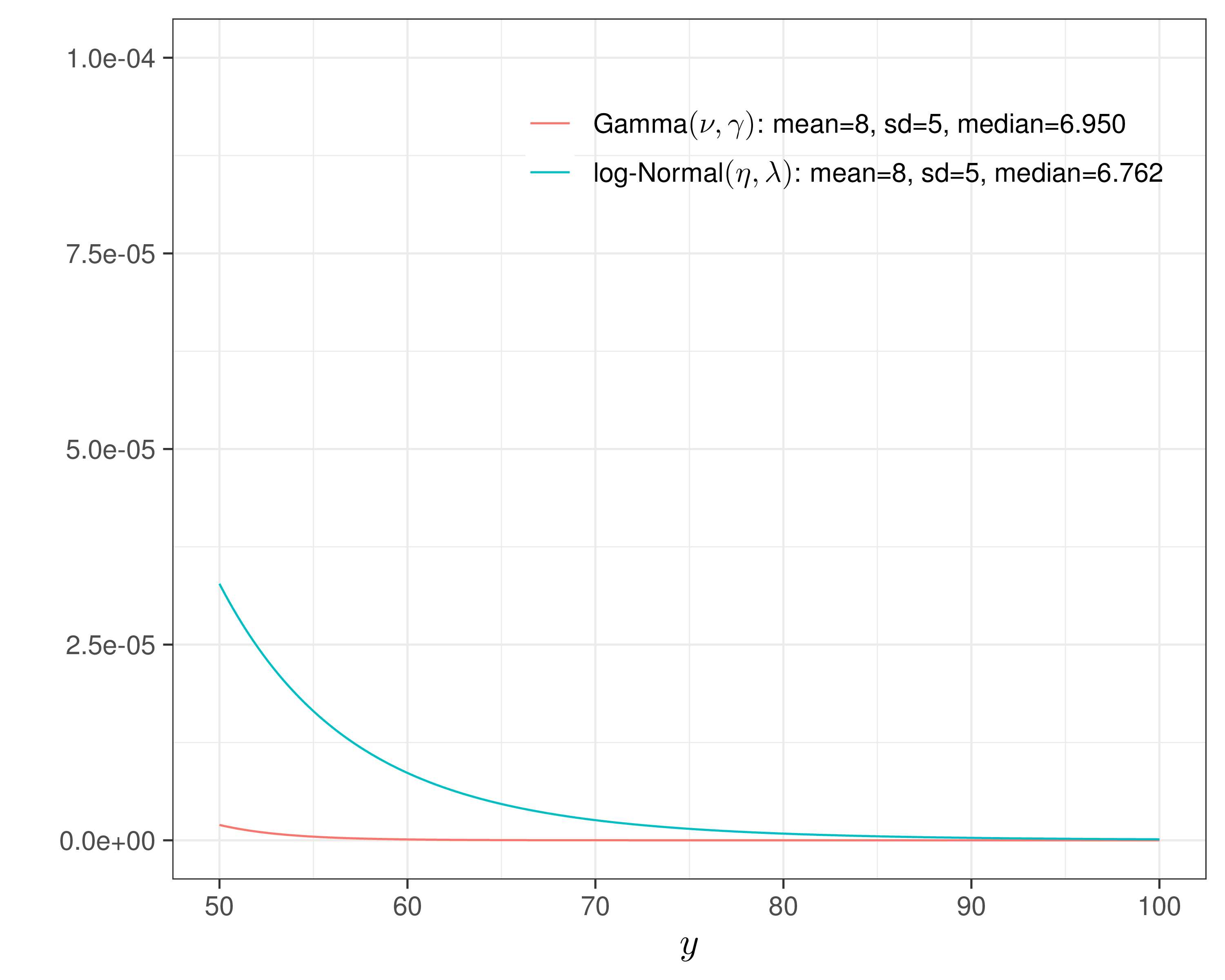
Costs usually skewed and benefits may be bounded in \([0; 1]\)
Can use transformation (e.g. logs) – but care is needed when back transforming to the natural scale
Should use more suitable models (e.g. Beta, Gamma or log-Normal) – (generally easier under a Bayesian framework)
Particularly relevant in presence of partially observed data – more on this later!
Particularly as the focus is on decision-making (rather than just inference), we need to use all available evidence to fully characterise current uncertainty on the model parameters and outcomes (Mainly ALD)
A Bayesian approach is helpful in combining different sources of information
(Propagating uncertainty is a fundamentally Bayesian operation!)
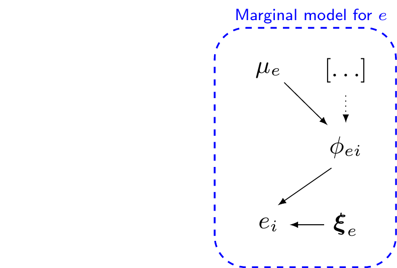
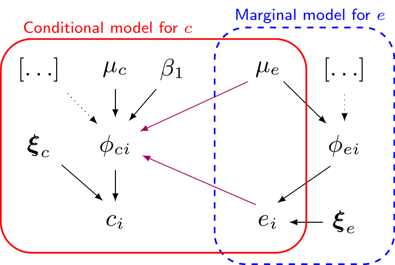
Marginal/conditional factorisation model
In general, can represent the joint distribution as \(\class{myblue}{p(e,c) = p(e)p(c\mid e) = p(c)p(e\mid c)}\)
Marginal/conditional factorisation model
In general, can represent the joint distribution as \(\class{myblue}{p(e,c) = }\class{blue}{p(e)}\class{myblue}{p(c\mid e) = p(c)p(e\mid c)}\)
In general, can represent the joint distribution as \(\class{myblue}{p(e,c) = }\class{blue}{p(e)}\class{red}{p(c\mid e)}\class{myblue}{ = p(c)p(e\mid c)}\)
Combining “modules” and fully characterising uncertainty about deterministic functions of random quantities is relatively straightforward using MCMC
Prior information can help stabilise inference (especially with sparse data!), eg
Cancer patients are unlikely to survive as long as the general population
ORs are unlikely to be greater than \(\pm \style{font-family:inherit;}{\text{5}}\)
To be or not to be?… (A Bayesian)
In principle, there’s nothing inherently Bayesian about MCF… BUT: there’s lots of advantages in doing it in a Bayesian setup
As the model becomes more and more realistic and its structure more and more complex, to account for skeweness and correlation, the computational advantages of using maximum likelihood estimations become increasingly smaller
Writing and optimising the likelihood function becomes more complex analytically and even numerically and might require the use of simulation althorithms
Bayesian models generally scale up with minimal changes
Computation may be more expensive, but the marginal computational cost is in fact diminishing
Realistic models are usually based on highly non-linear transformations
from a Bayesian perspective, this does not pose a substantial problem, because once we obtain simulations from the posterior distribution for \(\alpha_0\) and \(\beta_0\), it is possible to simply rescale them to obtain samples from the posterior distribution of \(\mu_e\) and \(\mu_c\)
This allows us to fully characterise and propagate the uncertainty in the fundamental economic parameters to the rest of the decision analysis with essentially no extra computational cost
Frequentist/ML approach would resort to resampling methods, such as the bootstrap to effectively produce an approximation to the joint posterior distribution for all the model parameters \(\bm\theta\) and any function thereof
Prior information can help stabilise inference
Most often, we do have contextual information to mitigate limited evidence from the data and stabilise the evidence
Using a Bayesian approach allows us to use this contextual information in a principled way.
# Normal/Normal MCF - JAGS codenn_mcf=function(){for (i in1:N) {# Marginal model for the effects e[i] ~dnorm(phi.e[i], tau.e[Trt[i]]) phi.e[i] <- alpha0 + alpha1*(Trt[i]-1) + alpha2*u0star[i]# *Conditional* model for the costs c[i] ~dnorm(phi.c[i], tau.c[Trt[i]]) phi.c[i] <- beta0 + beta1*(e[i]-mu.e[Trt[i]]) + beta2*(Trt[i]-1) }# Rescales the main economic parametersfor (t in1:2) { mu.e[t] <- alpha0 + alpha1*(t-1) mu.c[t] <- beta0 + beta2*(t-1) }# Minimally informative priors on the regression coefficients alpha0 ~dnorm(0,0.0001) alpha1 ~dnorm(0,0.0001) alpha2 ~dnorm(0,0.0001) beta0 ~dnorm(0,0.0001) beta1 ~dnorm(0,0.0001) beta2 ~dnorm(0,0.0001)for (t in1:2) {# PC-prior on the *marginal* sd with Pr(sigma_e>0.8) \approx 0.01 sigma.e[t] ~dexp(5.75) tau.e[t] <-pow(sigma.e[t],-2)# PC-prior on the *conditional* sd with Pr(lambda_c>100) \approx 0.1 lambda.c[t] ~dexp(0.025) tau.c[t] <-pow(lambda.c[t],-2)# Retrieves the correlation coefficients rho[t] <- beta1*sigma.e[t]/sigma.c[t]# And the *marginal* standard deviation for the cost sigma.c[t] <-sqrt(pow(lambda.c[t],2) +pow(sigma.e[t],2)*pow(beta1,2)) }}
Normal/Normal MCF — 10TT
Normal/Normal MCF — running JAGS
# Runs JAGS in the background and stores the output in the element 'nn_mcf' model$nn_mcf=jags(data=data,parameters.to.save=c("mu.e","mu.c","alpha0","alpha1","alpha2","beta0","beta1","beta2","sigma.e","sigma.c","lambda.c","rho" ),inits=NULL,n.chains=2,n.iter=5000,n.burnin=3000,n.thin=1,DIC=TRUE,# This specifies the model code as the function 'nn_mcf'model.file=nn_mcf)# Shows the summary statistics from the posterior distributions. print(model$nn_mcf,digits=3,interval=c(0.025,0.5,0.975))
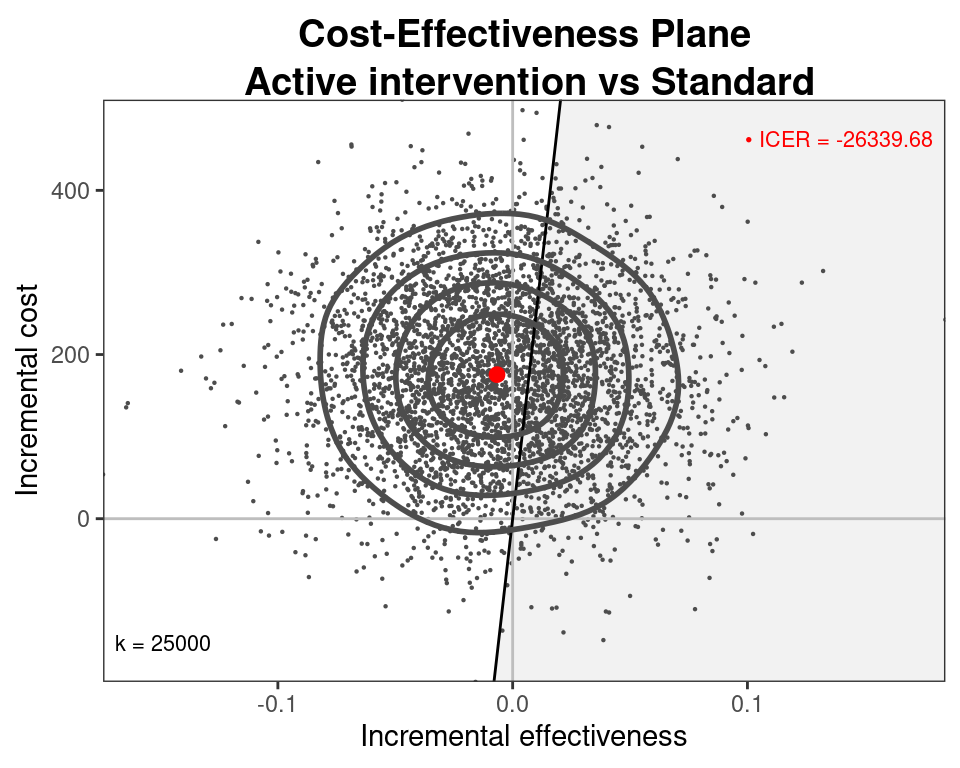
Normal/Normal independent vs Normal/Normal MCF — 10TT
Normal/Normal independentNormal/Normal MCF
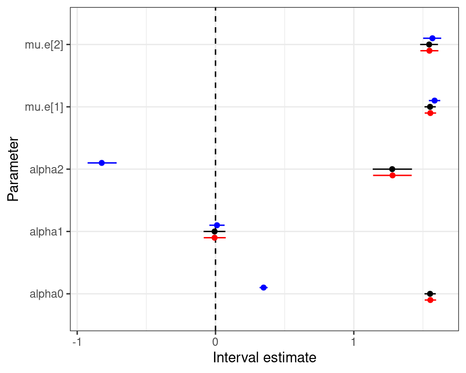
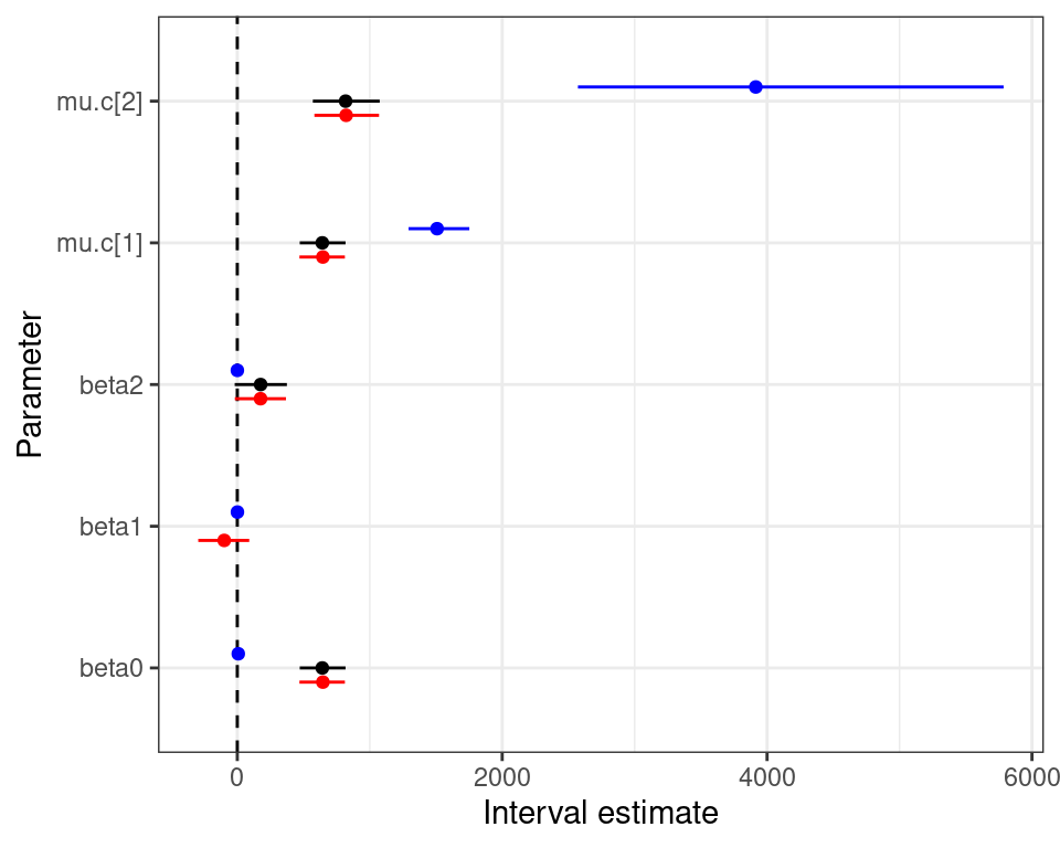
Data transformation
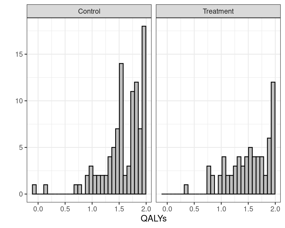
There’s a couple of complications with the effect data
Exhibit large left skewness
A small number of individuals are associated with negative QALYs, indicating a very poor health state (“worse than death”)
Easy solution: rescale and define
\[e^*_i = (3 -e_i)\]
This rescales the observed QALYs and turns the distribution into a right skewed, which means we can use a Gamma distribution to model the sampling variability
Gamma/Gamma MCF — 10TT
\[\begin{align*}
e^*_{i} \sim \dgamma (\nu_e,\gamma_{ei}) && & \log(\phi_{ei}) = \alpha_0 + \alpha_1(\text{Trt}_i - 1) + \alpha_2 u^*_{0i}\\
c_i\mid e^*_i \sim \dgamma(\nu_c,\gamma_{ci}) && & \log(\phi_{ci}) = \beta_0 + \beta_1(e^*_i -\mu^*_e) + \beta_2(\text{Trt}_i - 1),
\end{align*}\] where, because of the properties of the Gamma distribution
\(\phi_{ei}\) indicates the marginal mean for the QALYs,
\(\nu_e\) is the shape
\(\gamma_{ei}=\nu_c/\phi_{ei}\) is the rate
Similarly
\(\nu_c\) is the shape
\(\gamma_{ci}=\nu_c/\phi_{ci}\) is the rate of the conditional distribution for the costs given the benefits
\(\phi_{ci}\) is the conditional mean
Gamma/Gamma MCF — 10TT
Prior distributions
Keep the very vague, minimally informative priors for the regression coefficients
Again, we could probably do better here, considering that both \(\phi_{ei}\) and \(\phi_{ci}\) are defined on a log scale and thus we are implying a very large range in the priors
Sensitivity analysis may be very important to this aspect
As for the shape parameters \(\nu_{et}\) and \(\nu_{ct}\), we specify again a PC prior
Generally speaking, it is more difficult to encode genuine prior knowledge on this scale
Thus we start by including a fairly vague specification, where we assume that \(\Pr(\nu_{et}>30)=\Pr(\nu_{ct}>30)\approx 0.01\) — this implies an Exponential with rate \(-\frac{\log(0.01)}{30}\approx 0.15\)
Gamma/Gamma MCF — 10TT
Gamma/Gamma MCF — model code
# Gamma/Gamma MCF - JAGS codegg_mcf=function(){for (i in1:N) {# Marginal model for the *rescaled* effects estar[i] ~dgamma(nu.e[Trt[i]], gamma.e[Trt[i],i]) gamma.e[Trt[i],i] <- nu.e[Trt[i]]/phi.e[i]log(phi.e[i]) <- alpha0 + alpha1*(Trt[i]-1) + alpha2*u0star[i]# Conditional model for the costs c[i] ~dgamma(nu.c[Trt[i]], gamma.c[Trt[i],i]) gamma.c[Trt[i],i] <- nu.c[Trt[i]]/phi.c[i]log(phi.c[i]) <- beta0 + beta1*(estar[i]-mustar.e[Trt[i]]) + beta2*(Trt[i]-1) }# Rescales the main economic parametersfor (t in1:2) { mustar.e[t] <-exp(alpha0 + alpha1*(t-1)) mu.e[t] <-3- mustar.e[t] mu.c[t] <-exp(beta0 + beta1*(t-1)) }# Minimally informative priors on the regression coefficients alpha0 ~dnorm(0,0.0001) alpha1 ~dnorm(0,0.0001) alpha2 ~dnorm(0,0.0001) beta0 ~dnorm(0,0.0001) beta1 ~dnorm(0,0.0001) beta2 ~dnorm(0,0.0001)# PC prior on the shape parameters # assume that Pr(nu.e>30) = Pr(nu.c>30) \approx 0.01for (t in1:2) { nu.e[t] ~dexp(0.15) nu.c[t] ~dexp(0.15) }}
Gamma/Gamma MCF — 10TT
Gamma/Gamma MCF — running JAGS
# Defines the rescaled QALYs in the data list and remove the old versiondata$estar=3-data$e# Runs JAGS in the background and stores the output in the element 'gg_mcf' model$gg_mcf=jags(data=data,parameters.to.save=c("mu.e","mustar.e","mu.c","alpha0","alpha1","alpha2","beta0","beta1","beta2","nu.e","nu.c" ),inits=NULL,n.chains=2,n.iter=5000, n.burnin=3000,n.thin=1,DIC=TRUE,# This specifies the model code as the function 'model.code'model.file=gg_mcf)# Shows the summary statistics from the posterior distributions. print(model$gg_mcf,digits=3,interval=c(0.025,0.5,0.975))
\[\displaystyle\dic=p_D + \overline{D(\bm\theta)} = D(\overline{\bm\theta})+2p_d,\] where
\(\class{myblue}{\displaystyle\overline{D(\bm\theta)} =\E\left[D(\bm\theta)\right] = \int -2\log\mathcal{L}(\bm\theta\mid\bm{y})p(\bm\theta\mid\bm{y})d\bm\theta \approx \frac{1}{S}\sum_{s=1}^S -2\log \mathcal{L}(\bm\theta^{(s)})} =\) average model deviance
\(\class{myblue}{\displaystyle D(\overline{\bm\theta})=D(\E\left[\bm\theta\mid\bm{y}\right]) = -2\log\mathcal{L}\left(\int \bm\theta p(\bm\theta\mid\bm{y})d\bm\theta \right) \approx -2\log \mathcal{L} \left( \frac{1}{S}\sum_{s=1}^S \bm\theta^{(s)} \right)}=\) model deviance calculated in correspondence of the average value of the model parameters
\(\class{myblue}{\displaystyle p_D=\overline{D(\bm\theta)}-D(\overline{\bm\theta})}=\) penalty for model complexity