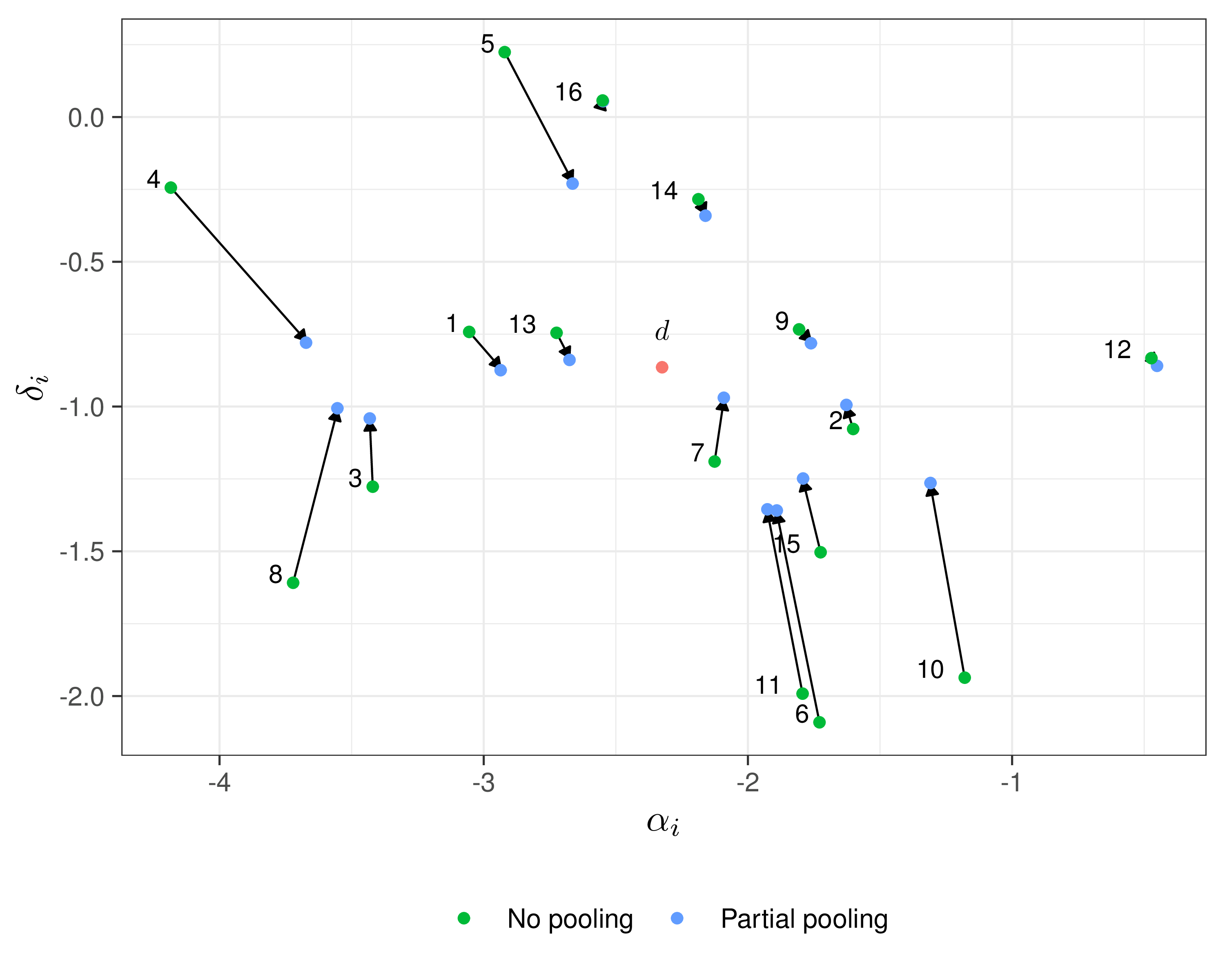
| Placebo | Magnesium | |||||
|---|---|---|---|---|---|---|
| ID | Name | Year | Deaths \((r_1)\) | Total \((n_1)\) | Deaths \((r_2)\) | Total \((n_2)\) |
| 1 | Morton | 1984 | 2 | 36 | 1 | 40 |
| 2 | Rasmussen | 1986 | 23 | 135 | 9 | 135 |
| 3 | Smith | 1986 | 7 | 200 | 2 | 200 |
| 4 | Abraham | 1987 | 1 | 46 | 1 | 48 |
| 5 | Felstedt | 1988 | 8 | 148 | 10 | 150 |
| 6 | Shechter | 1989 | 9 | 56 | 1 | 59 |
| 7 | Ceremuzynski | 1989 | 3 | 23 | 1 | 25 |
| 8 | Bertschat | 1989 | 1 | 21 | 0 | 22 |
| 9 | Singh | 1990 | 11 | 75 | 6 | 76 |
| 10 | Pereira | 1990 | 7 | 27 | 1 | 27 |
| 11 | Shechter 1 | 1991 | 12 | 80 | 2 | 89 |
| 12 | Golf | 1991 | 13 | 33 | 5 | 23 |
| 13 | Thorgersen | 1991 | 8 | 122 | 4 | 130 |
| 14 | LIMIT-2 | 1992 | 118 | 1157 | 90 | 1159 |
| 15 | Shechter 2 | 1995 | 17 | 108 | 4 | 107 |
| 16 | ISIS-4 | 1995 | 2103 | 29039 | 2216 | 29011 |
4. Aggregated level data and evidence synthesis
Department of Statistical Science | University College London
https://gianluca.statistica.it
https://egon.stats.ucl.ac.uk/research/statistics-health-economics
https://github.com/giabaio https://github.com/StatisticsHealthEconomics
@gianlubaio@mas.to @gianlubaio
Bayesian modelling for economic evaluation of healthcare interventions
València International Bayesian Analysis Summer School, 7th edition, University of Valencia
10 - 11 July 2024
Check out our departmental podcast “Random Talks” on Soundcloud!
Follow our departmental social media accounts + magazine “Sample Space”
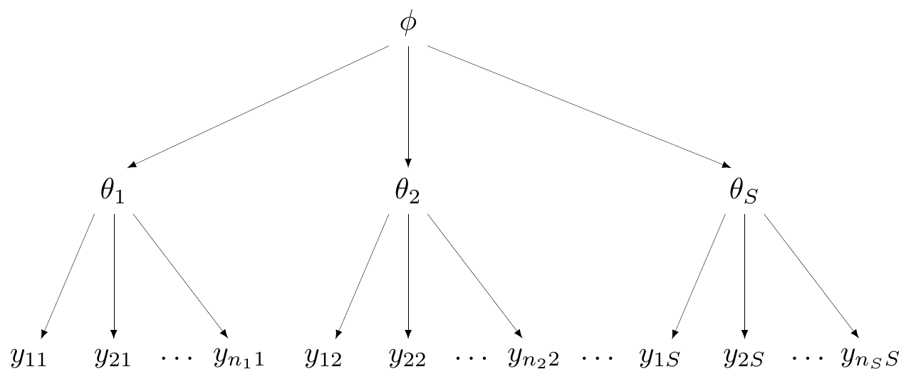
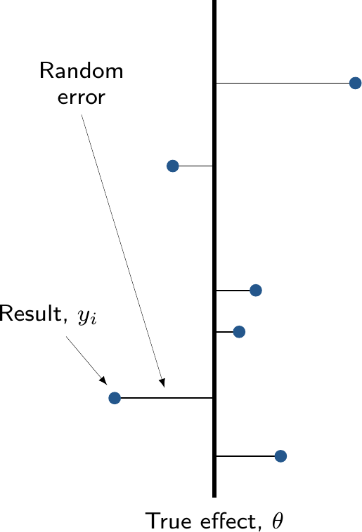
No pooling
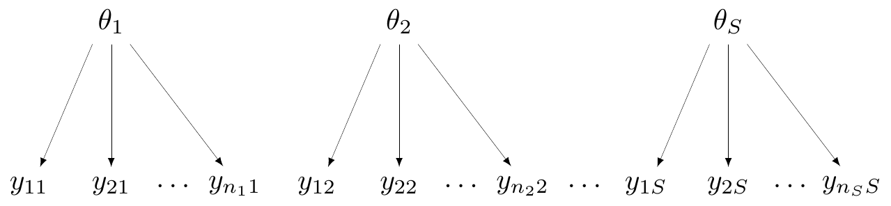
- All groups (e.g. “studies”) are assumed independent
- Not much use for economic modelling, unless only a single study is relevant
No pooling
- In Magnesium example, assume \(\alpha_i, \delta_i \stackrel{iid}{\sim}\dnorm(0,sd)\)
NB: \(\pi_i\) is just a logical node and used for ease of notation — but can equivalently write \[\class{myblue}{r_i \sim \dbin({\class{red}{\underbrace{\class{myblue}{\logit^{-1}(\alpha_i + \delta_i \text{Trt}_i)}}_{\pi_i}}},n_i)}\]
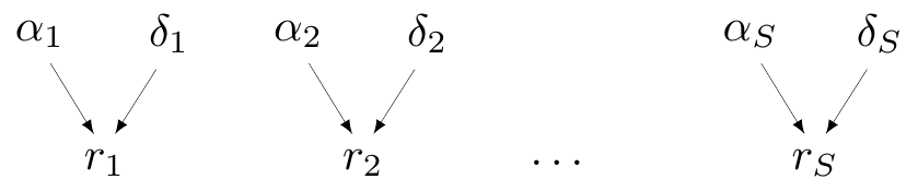
Complete pooling
- Assumes that all studies (and all data points!) are exchangeable
- They are “similar” — all come from the same data generating process
- DGP depends on a single parameter \(\theta\)
Complete pooling
- In Magnesium example, assume there is a common effect, \(\class{myblue}{\delta_i=d}\) for all \(i=1,\ldots,S\)
Technically, \(\alpha_i\) do vary by study, but they are some kind of “background noise” (the baseline) — the main parameter indicating the treatment effect is the common \(d\)
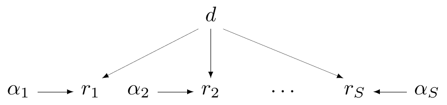
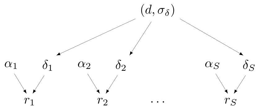
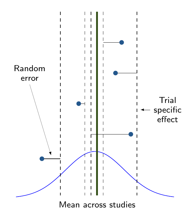
Partial pooling (hierarchical models)
- Data contribute to individual group estimate, but also to overall (pooled) estimate
Partial pooling (hierarchical models)
- In Magnesium example, assume
- \(\delta_i \sim \dnorm(d,\sigma_\delta)\)
- \(d \sim \dnorm(0,sd)\)
- \(\sigma_\delta \sim p(\sigma_\delta)\)
Complete vs partial pooling
Complete pooling
Partial pooling
Example — Magnesium
- Need to specify priors for \(\alpha_i,\delta_i\)
- Could assume \(sd \rightarrow \infty\) to ensure “no influence of the prior”…
- That’s overly cautious and unnecessary!
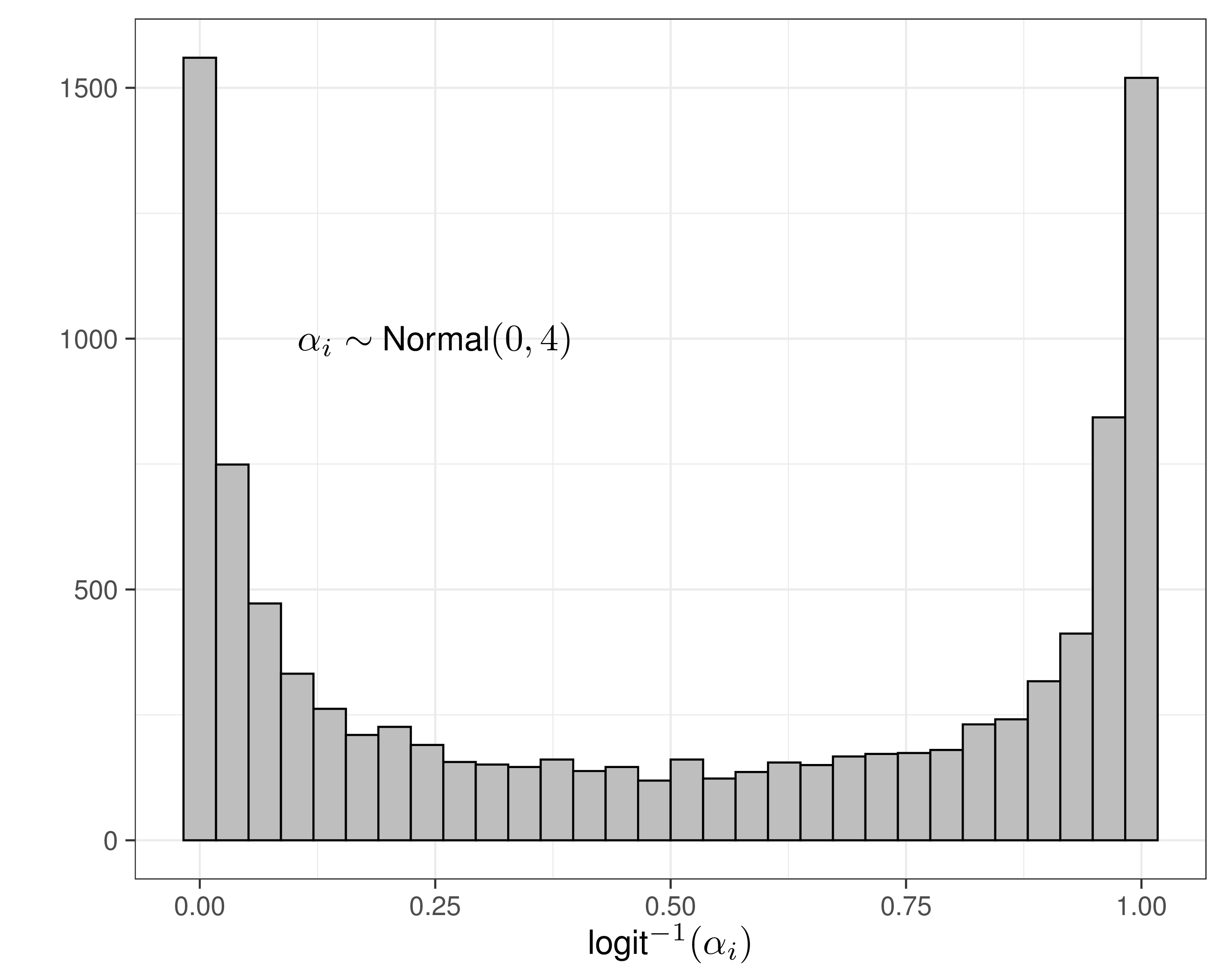
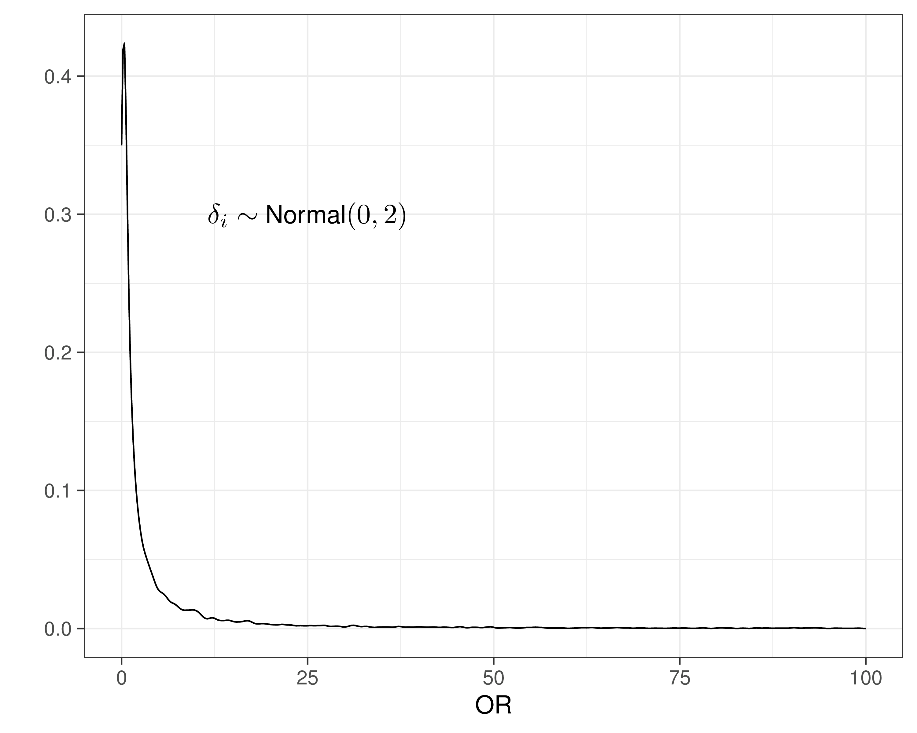
- These are modelled on the logit scale, so can use much smaller values for \(sd\) and still not imply too much information in the prior!
Example — Magnesium
Model comparison
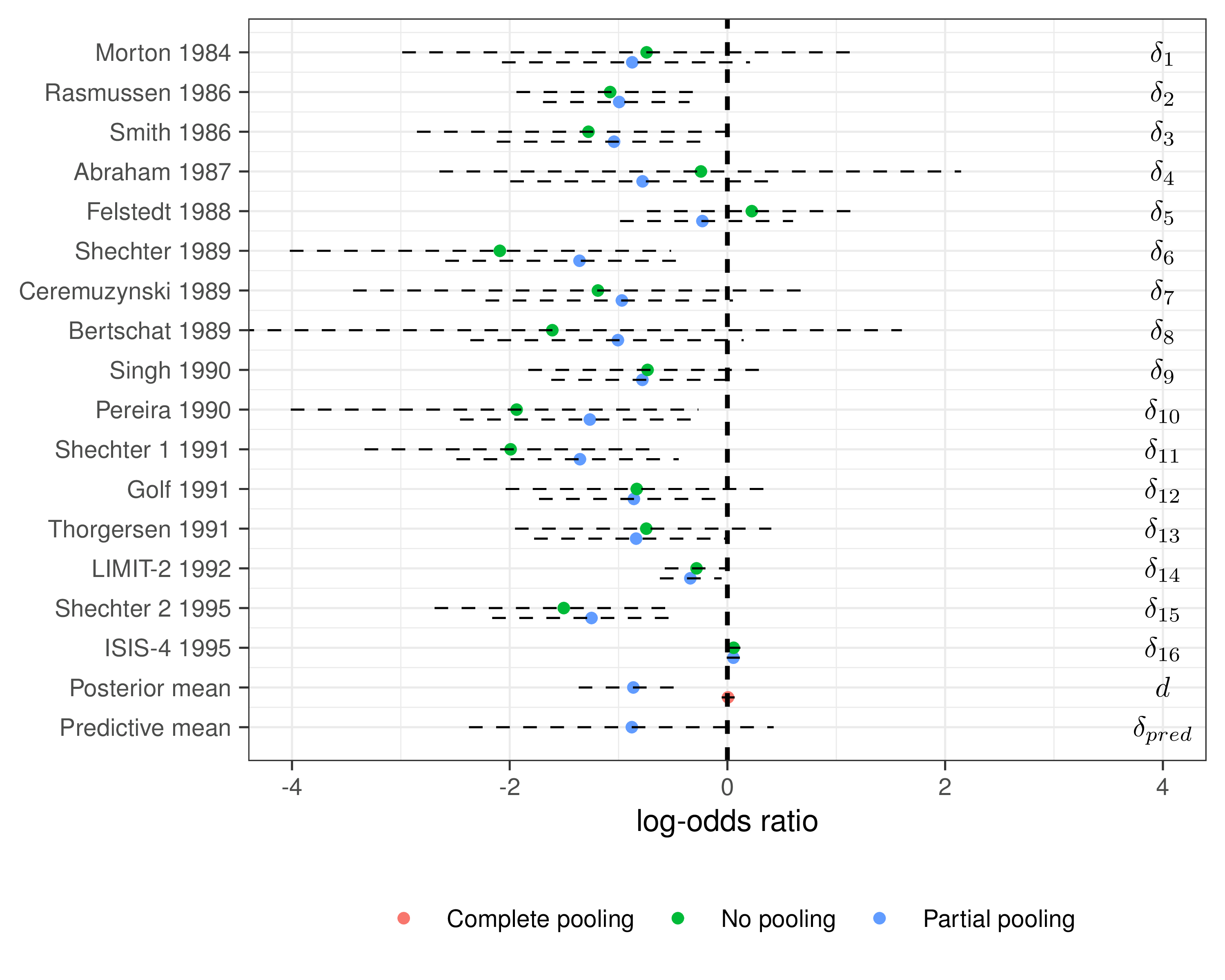
Example — Magnesium
Shrinkage
(“Standard”) cost-effectiveness modelling
- Build a population level model (e.g. decision tree or Markov model)
- NB: in this case, the “data” are typically represented by summary statistics for the parameters of interest \(\bm\theta=(p_0,p_1,l,\ldots)\), but may also have access to a combination of ILD and summaries
- Use point estimates for the parameters to build the “base-case” (average) evaluation
- Use resampling methods (eg bootstrap) to propage uncertainty in the point estimates and perform uncertainty analysis
Bayesian cost-effectiveness modelling
- Build a population level model (e.g. decision tree or Markov model)

- NB: in this case, the “data” are typically represented by summary statistics for the parameters of interest \(\bm\theta=(p_0,p_1,l,\ldots)\), but may also have access to a combination of ILD and summaries
- Estimate all model parameters at once and obtain MCMC simulations to run PSA and decision analysis at once
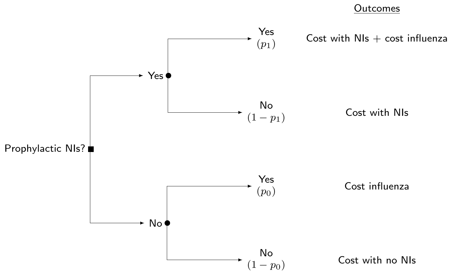
Cost-effectiveness analysis
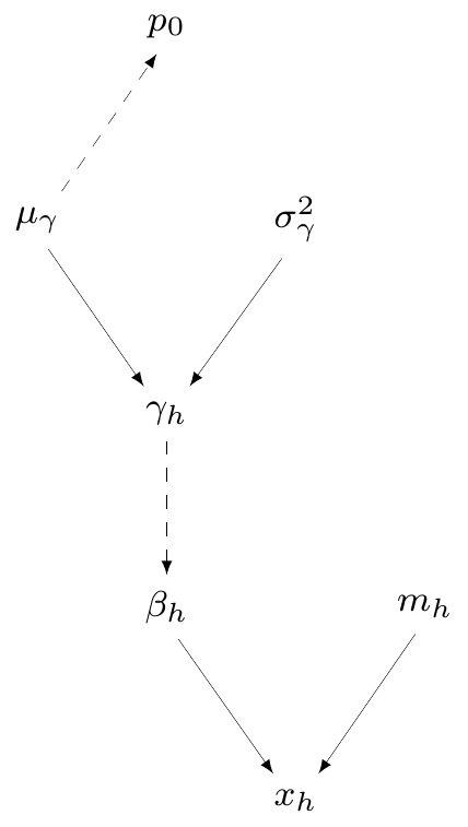
Module 1: Influenza incidence
\(H\) studies reporting number of patients who get influenza (\(x_h\)) in the sample (\(m_h\))
\(\beta_h=\) population probability of influenza from the \(h\)-th study: \(\logit(\beta_h)=\gamma_h\sim \dnorm(\mu\gamma,\sigma_\gamma)\)
\(\mu_\gamma\sim\dnorm(0,v)\) \(=\) pooled averaged probability of infection (on logit scale!) \(\Rightarrow \displaystyle \class{red}{p_0=\frac{\exp(\mu_\gamma)}{1+\exp(\mu_\gamma)}}\)
— or equivalently \(\class{red}{\logit(p_0)=\mu_\gamma}\)
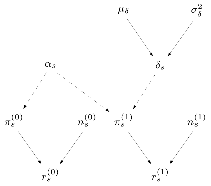
Cost-effectiveness analysis
Module 2: Prophylaxis effectiveness
\(S\) studies reporting number of infected patients \(r^{(t)}_s\) in a sample made of \(n^{(t)}_s\) subjects
\(\pi^{(t)}_s=\) study- and treatment-specific chance of contracting influenza
\(\logit\left(\pi^{(0)}_s\right) = \alpha_s \sim \dnorm(0, 10)\)
\(\logit\left(\pi^{(1)}_s\right) = \alpha_s + \delta_s\)
\(\delta_s \sim \dnorm(\mu_\delta,\sigma_\delta)=\) study-specific treatment effect
\(\class{blue}{\mu_\delta\sim\dnorm(0,v)}=\) pooled log-odds ratio of influenza given treatment
Cost-effectiveness analysis
Decision analytic model
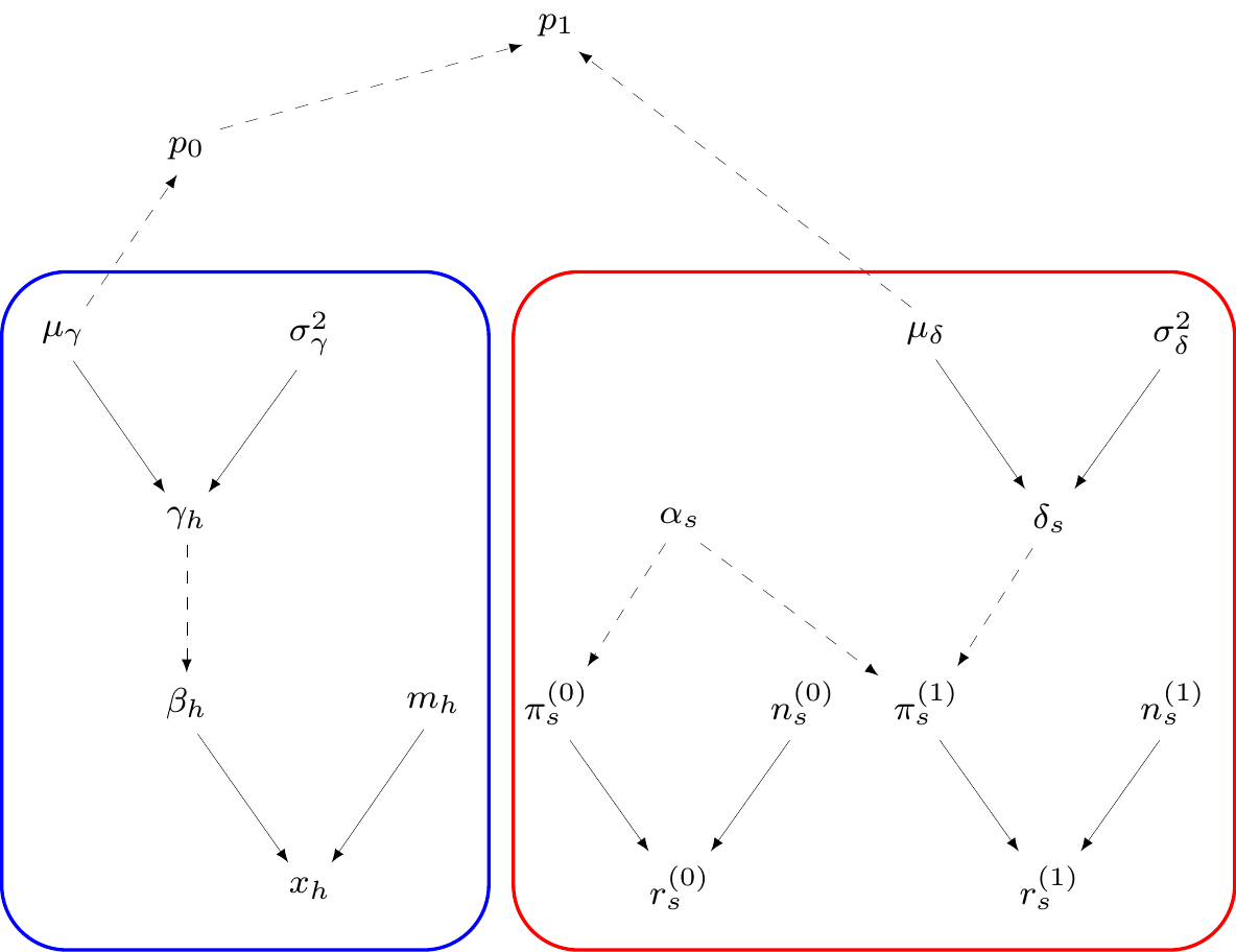
Can combine modules 1 and 2 to get \(\class{olive}{\logit(p_1)=\logit(p_0)+\mu_\delta}\)