1. Introduction to health economic evaluation
Department of Statistical Science | University College London
https://gianluca.statistica.it
https://egon.stats.ucl.ac.uk/research/statistics-health-economics
https://github.com/giabaio https://github.com/StatisticsHealthEconomics
@gianlubaio@mas.to @gianlubaio
Bayesian modelling for economic evaluation of healthcare interventions
València International Bayesian Analysis Summer School, 7th edition, University of Valencia
10 - 11 July 2024
Check out our departmental podcast “Random Talks” on Soundcloud!
Follow our departmental social media accounts + magazine “Sample Space”
Disclaimer…

… Just so you know what you’re about to get yourself into… 😉
Health technology assessment (HTA)
Objective
- Combine costs and benefits of a given intervention into a rational scheme for allocating resources
Health technology assessment (HTA)
Objective
- Combine costs and benefits of a given intervention into a rational scheme for allocating resources
To be or not to be?… (A Bayesian)
Frequentist (“standard”)
Bayesian
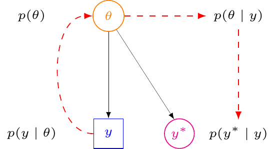
- A Bayesian only speaks one language: probability distributions to describe
- Sampling variability (relevant for observed data)
- Epistemic uncertainty (relevant for unobservable parameters + yet unobserved future data)
- Contextual (=“prior”) information to be formally included in the construction of the model
- Almost irrelevant when evidence is “definitive” (large and consistent data)
- Crucial when data are sparse!
- Almost irrelevant when evidence is “definitive” (large and consistent data)
To be or not to be?… (A Bayesian)
In HTA
Frequentist (“standard”)
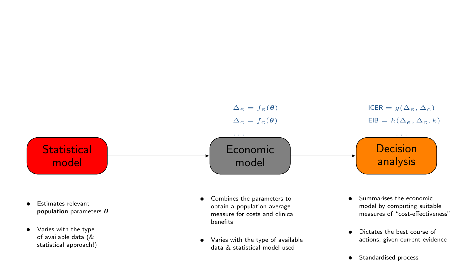
2./3. Economic modelling+Decision analysis
Base-case scenario
\[\class{myblue}{\Delta_e=}\class{red}{\underbrace{\class{myblue}{\E[e \mid \boldsymbol{\hat\theta}_1]}}_{\class{red}{\hat\mu_{e1}}}} \class{myblue}{-} \class{red}{\underbrace{\class{myblue}{\E[e \mid \boldsymbol{\hat\theta}_0]}}_{\class{red}{\hat\mu_{e0}}}}\]
\[\class{myblue}{\Delta_c=}\class{red}{\underbrace{\class{myblue}{\E[c \mid \boldsymbol{\hat\theta}_1]}}_{\class{red}{\hat\mu_{c1}}}} \class{myblue}{-} \class{red}{\underbrace{\class{myblue}{\E[c \mid \boldsymbol{\hat\theta}_0]}}_{\class{red}{\hat\mu_{c0}}}}\]
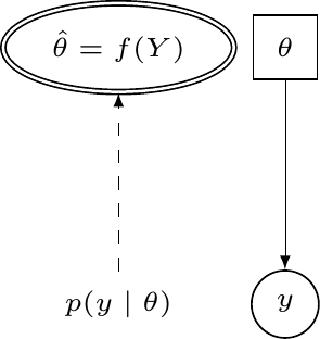
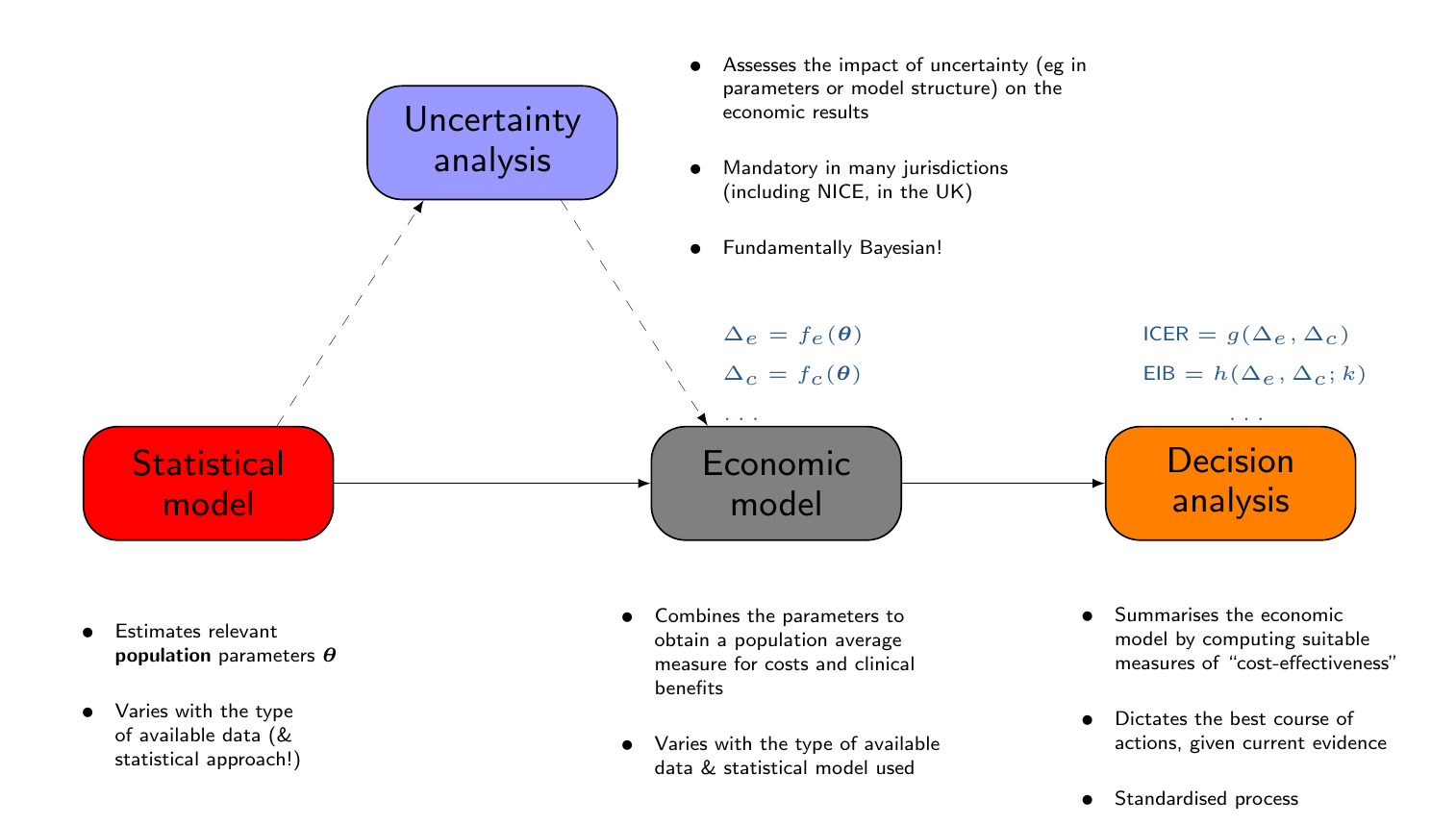
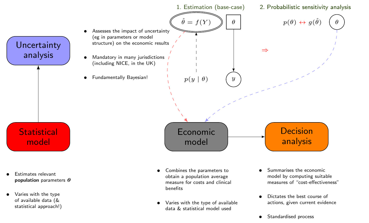
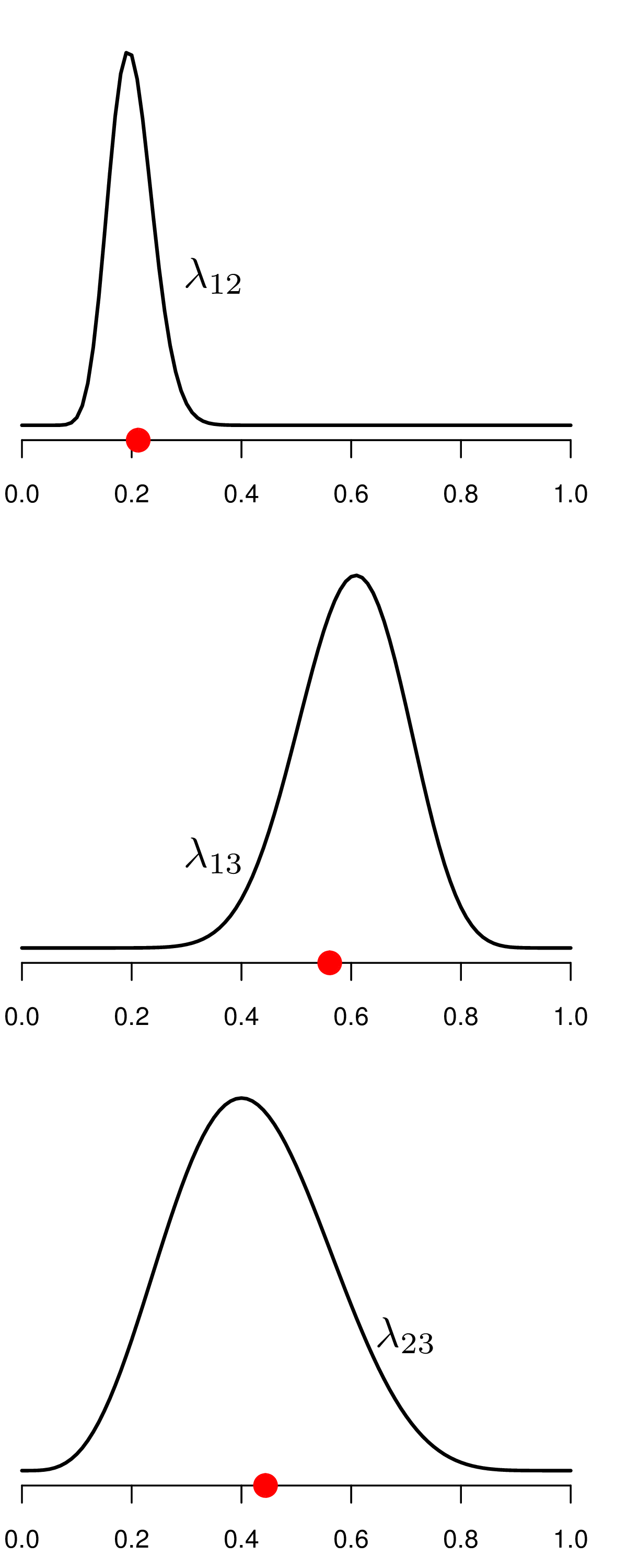
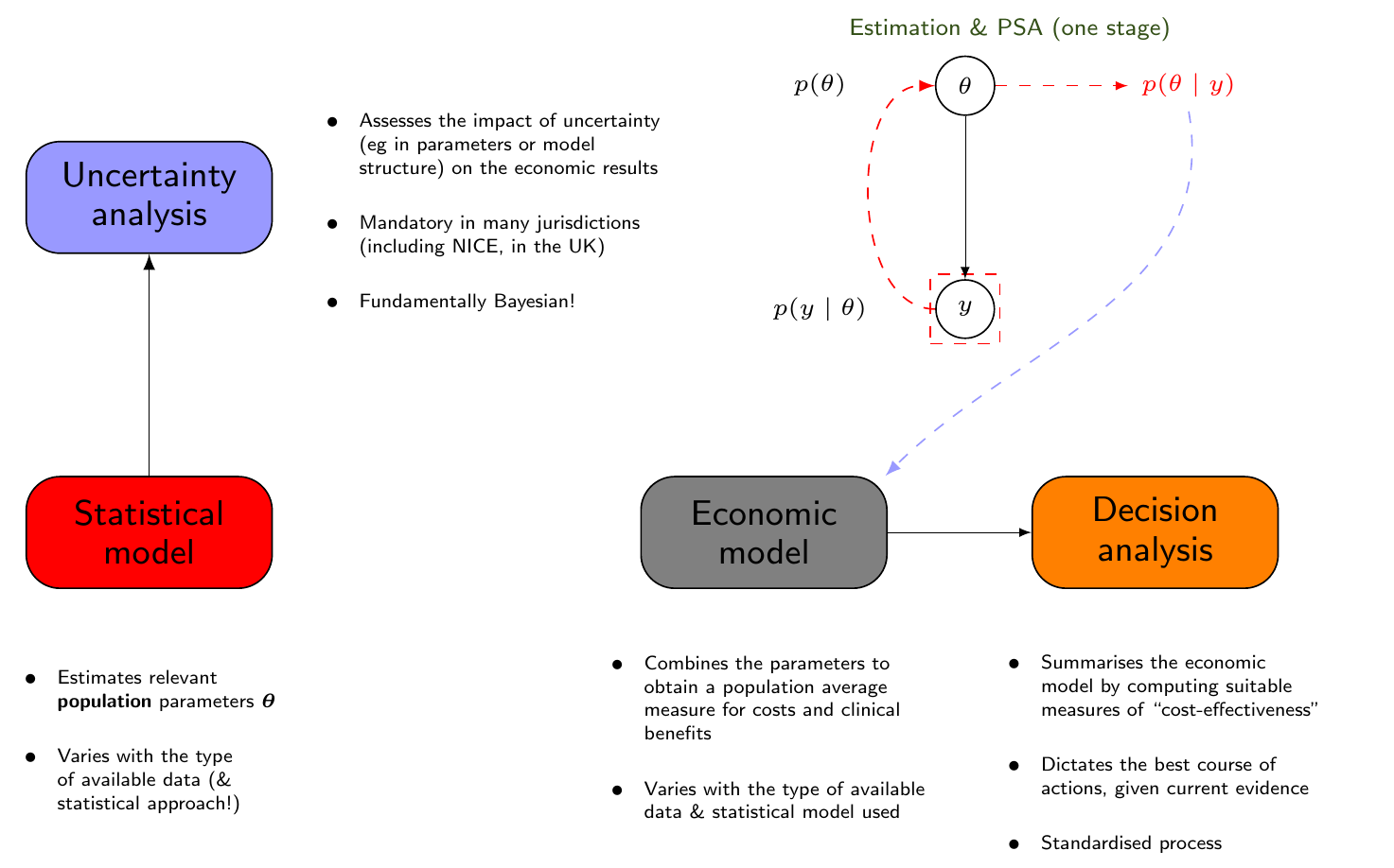
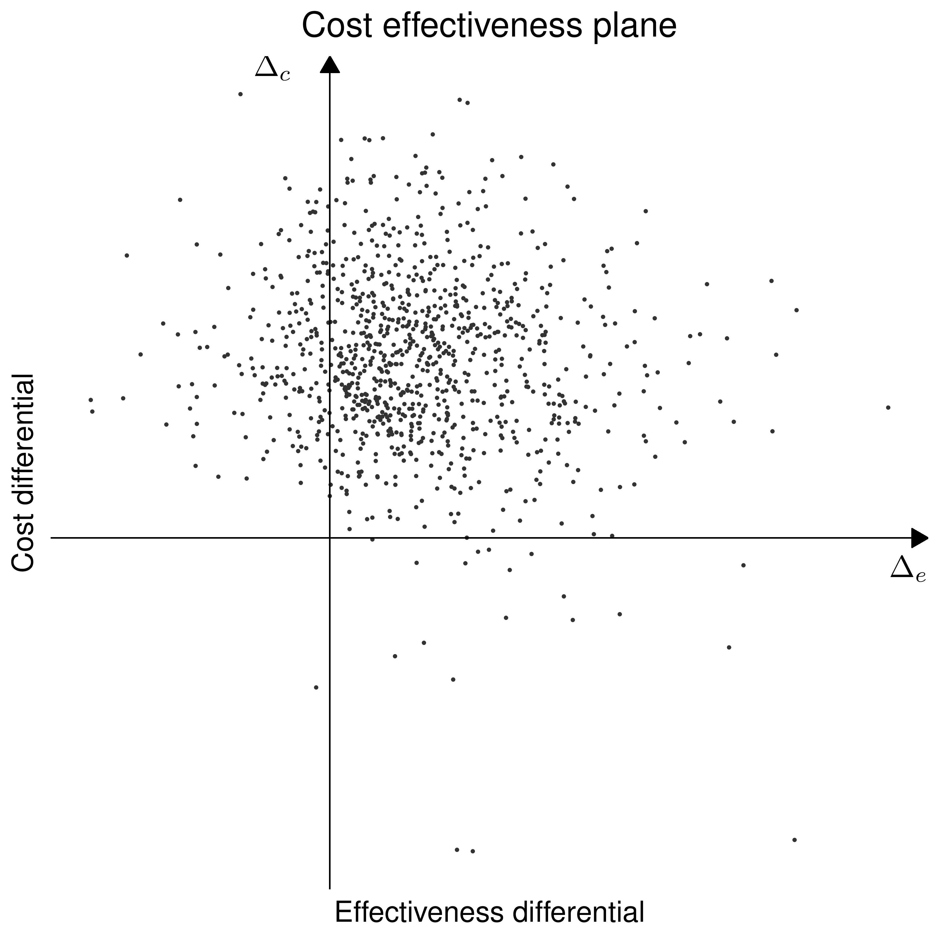
4. Uncertainty analysis
Uncertainty induced by \(g(\boldsymbol{\hat\theta}_0),g(\boldsymbol{\hat\theta}_1)\) — typically independent simulations
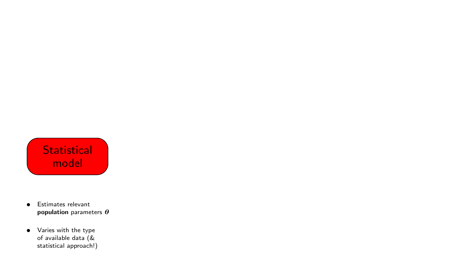
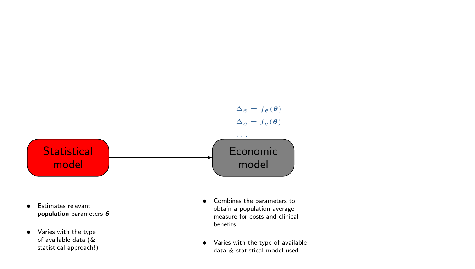
Statistical model

Economic model
Status quo
New drug
Decision analysis
| Benefits | Costs |
|---|---|
| 741 | 670382.1 |
| 699 | 871273.3 |
| ... | ... |
| 726 | 425822.2 |
| 716.2 | 790381.2 |
| Benefits | Costs |
|---|---|
| 732 | 1131978 |
| 664 | 1325654 |
| ... | ... |
| 811 | 766411.4 |
| 774.5 | 1066849.8 |
4. Uncertainty analysis
Uncertainty induced by \(g(\boldsymbol{\hat\theta}_0),g(\boldsymbol{\hat\theta}_1)\) — typically independent simulations
Statistical model
Economic model
Status quo
New drug
Decision analysis
| Benefits | Costs |
|---|---|
| 741 | 670382.1 |
| 699 | 871273.3 |
| ... | ... |
| 726 | 425822.2 |
| 716.2 | 790381.2 |
| Benefits | Costs |
|---|---|
| 732 | 1131978 |
| 664 | 1325654 |
| ... | ... |
| 811 | 766411.4 |
| 774.5 | 1066849.8 |
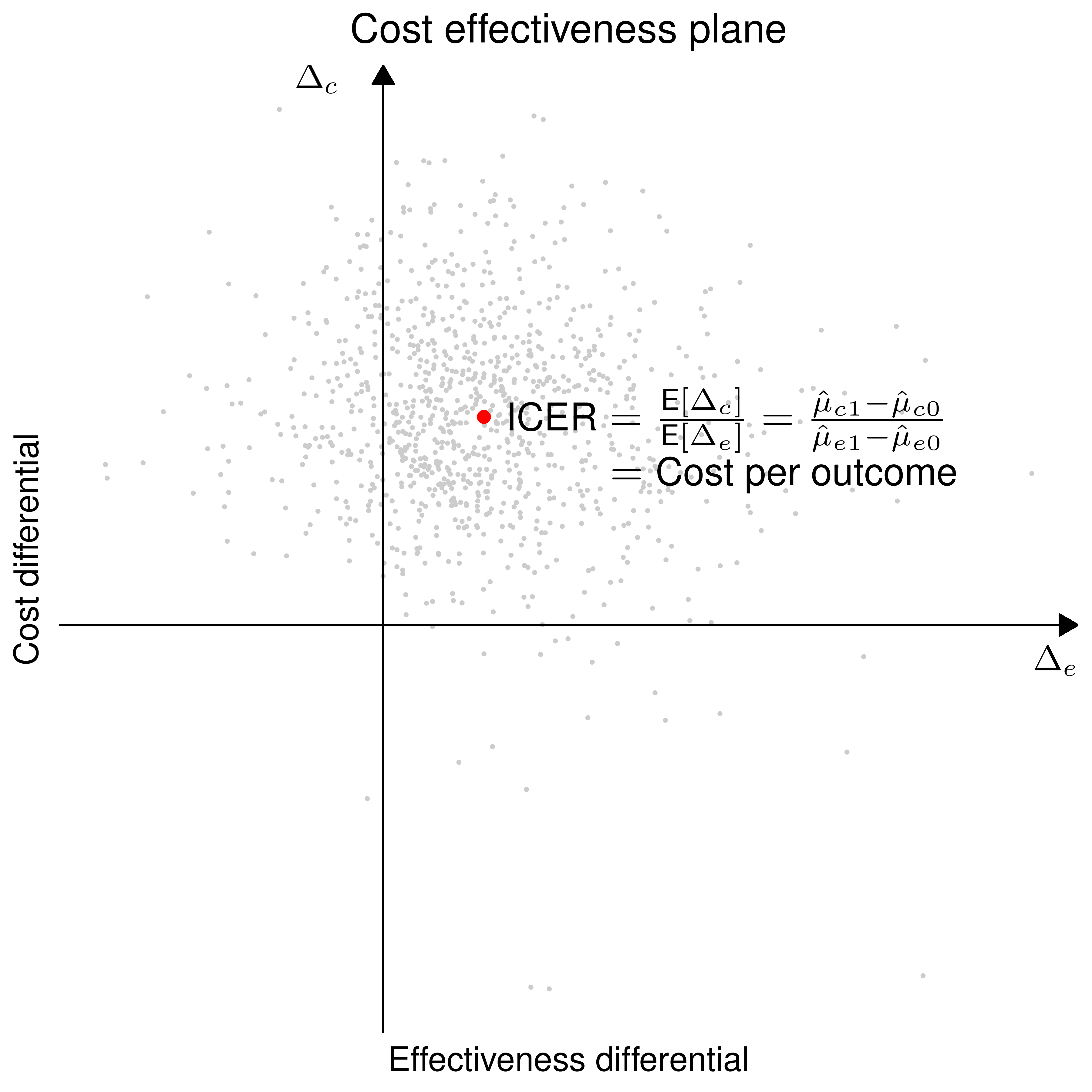
\[ \begin{align} \class{myblue}{\style{font-family:inherit;}{\text{ICER}}} & \class{myblue}{=} \frac{\class{myblue}{\style{font-family:inherit;}{\text{276468.6}}}}{\class{myblue}{\style{font-family:inherit;}{\text{58.3}}}}\\ & \class{myblue}{= \style{font-family:inherit;}{\text{6497.1}}} \end{align} \]
4. Uncertainty analysis*
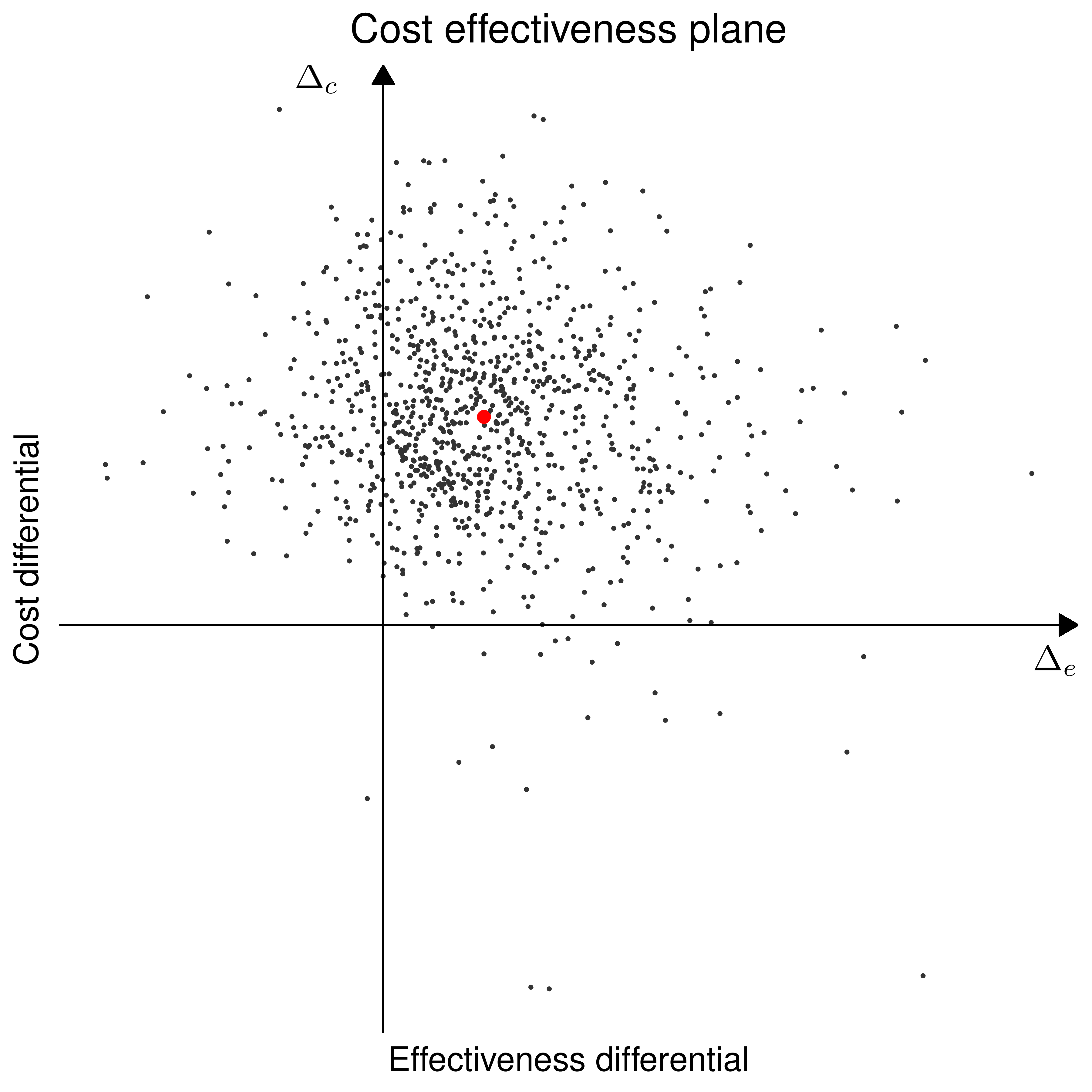
\[\class{myblue}{\Delta_e=}\class{red}{\underbrace{\class{myblue}{\E[e \mid \boldsymbol{\theta}_1]}}_{\class{red}{\mu_{e1}}}} \class{myblue}{-} \class{red}{\underbrace{\class{myblue}{\E[e \mid \boldsymbol{\theta}_0]}}_{\class{red}{\mu_{e0}}}}\]
\[\class{myblue}{\Delta_c=}\class{red}{\underbrace{\class{myblue}{\E[c \mid \boldsymbol{\theta}_1]}}_{\class{red}{\mu_{c1}}}} \class{myblue}{-} \class{red}{\underbrace{\class{myblue}{\E[c \mid \boldsymbol{\theta}_0]}}_{\class{red}{\mu_{c0}}}}\]
*Induced by \(\class{myblue}{g(\boldsymbol{\hat\theta}_0),g(\boldsymbol{\hat\theta}_1)}\)
To be or not to be?… (A Bayesian)
In HTA
Frequentist (“standard”)
Bayesian
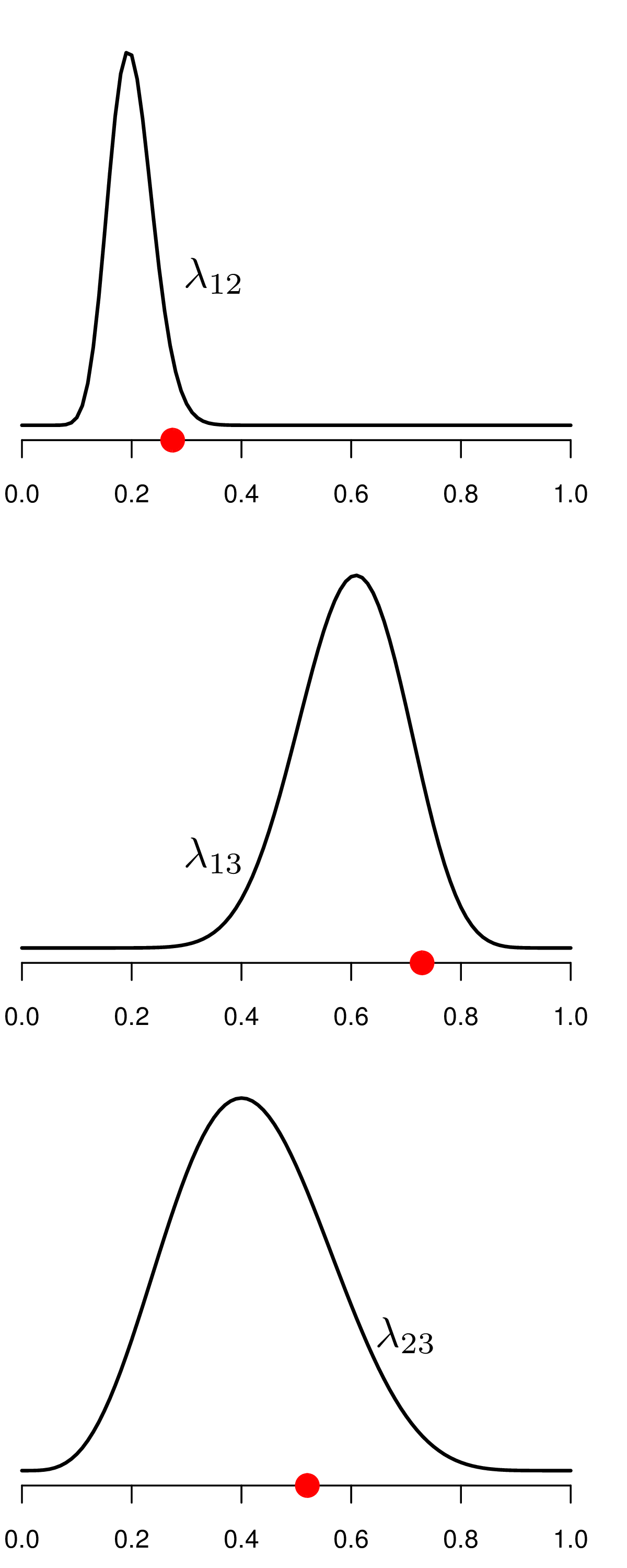
4. Uncertainty analysis
Uncertainty induced by \(\class{myblue}{p(\boldsymbol\theta\mid \txt{data})}\) — uses the joint posterior of all the parameters!
Statistical model
Economic model
Status quo
New drug
Decision analysis
| Benefits | Costs |
|---|---|
| 741 | 670382.1 |
| 699 | 871273.3 |
| ... | ... |
| 726 | 425822.2 |
| 716.2 | 790381.2 |
| Benefits | Costs |
|---|---|
| 732 | 1131978 |
| 664 | 1325654 |
| ... | ... |
| 811 | 766411.4 |
| 774.5 | 1066849.8 |
\[ \begin{align} \class{myblue}{\style{font-family:inherit;}{\text{ICER}}} & \class{myblue}{=} \frac{\class{myblue}{\style{font-family:inherit;}{\text{276468.6}}}}{\class{myblue}{\style{font-family:inherit;}{\text{58.3}}}}\\ & \class{myblue}{= \style{font-family:inherit;}{\text{6497.1}}} \end{align} \]
2./4. Economic model + Uncertainty analysis*
\[\class{myblue}{\Delta_e=}\class{red}{\underbrace{\class{myblue}{\E[e \mid \boldsymbol{\theta}_1]}}_{\class{red}{\mu_{e1}}}} \class{myblue}{-} \class{red}{\underbrace{\class{myblue}{\E[e \mid \boldsymbol{\theta}_0]}}_{\class{red}{\mu_{e0}}}}\]
\[\class{myblue}{\Delta_c=}\class{red}{\underbrace{\class{myblue}{\E[c \mid \boldsymbol{\theta}_1]}}_{\class{red}{\mu_{c1}}}} \class{myblue}{-} \class{red}{\underbrace{\class{myblue}{\E[c \mid \boldsymbol{\theta}_0]}}_{\class{red}{\mu_{c0}}}}\]
*Induced by \(\class{myblue}{p(\boldsymbol{\theta} \mid \style{font-family:inherit;}{\text{data}})}\)
3. Decision analysis
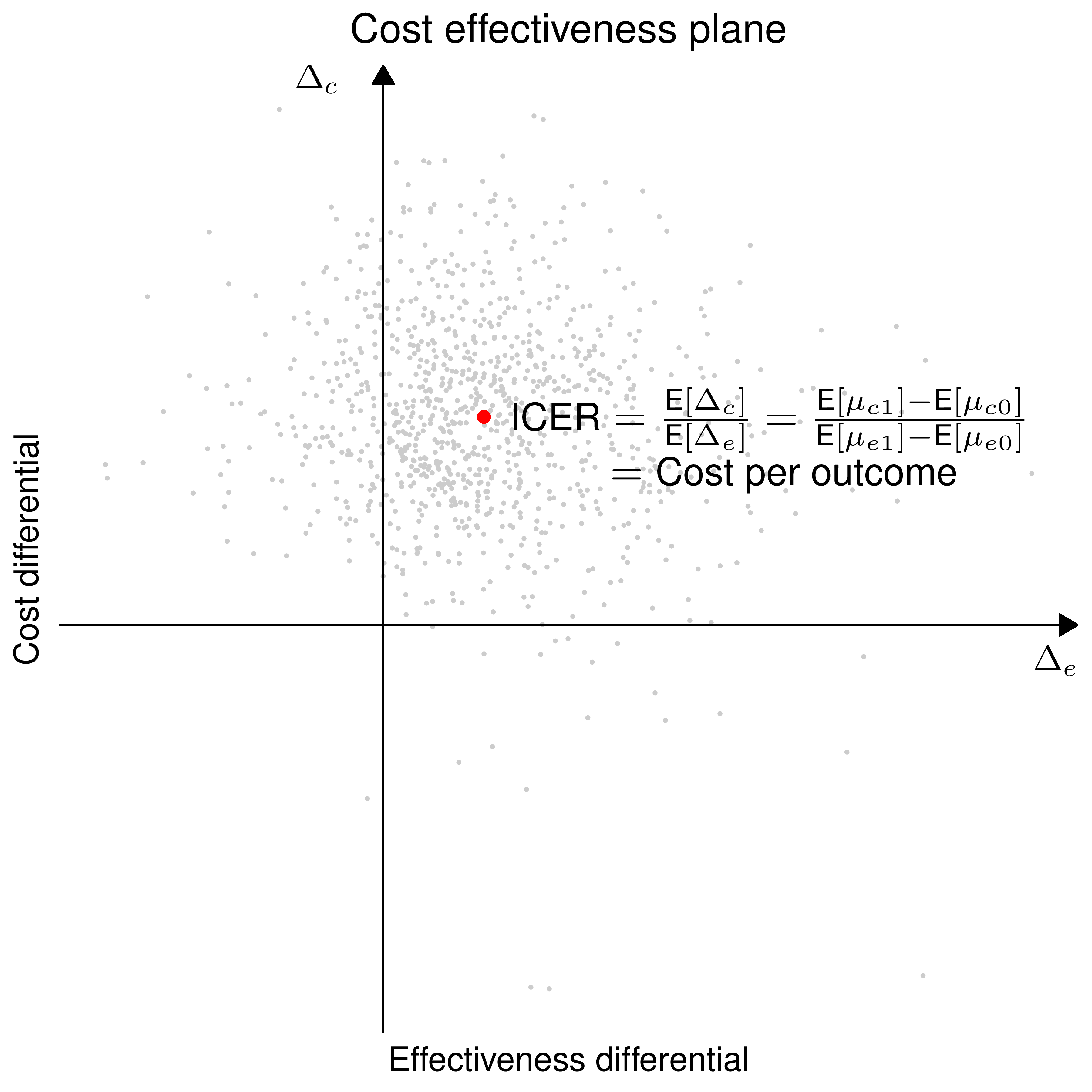
\[\class{myblue}{\Delta_e=}\class{red}{\underbrace{\class{myblue}{\E[e \mid \boldsymbol{\theta}_1]}}_{\class{red}{\mu_{e1}}}} \class{myblue}{-} \class{red}{\underbrace{\class{myblue}{\E[e \mid \boldsymbol{\theta}_0]}}_{\class{red}{\mu_{e0}}}}\]
\[\class{myblue}{\Delta_c=}\class{red}{\underbrace{\class{myblue}{\E[c \mid \boldsymbol{\theta}_1]}}_{\class{red}{\mu_{c1}}}} \class{myblue}{-} \class{red}{\underbrace{\class{myblue}{\E[c \mid \boldsymbol{\theta}_0]}}_{\class{red}{\mu_{c0}}}}\]
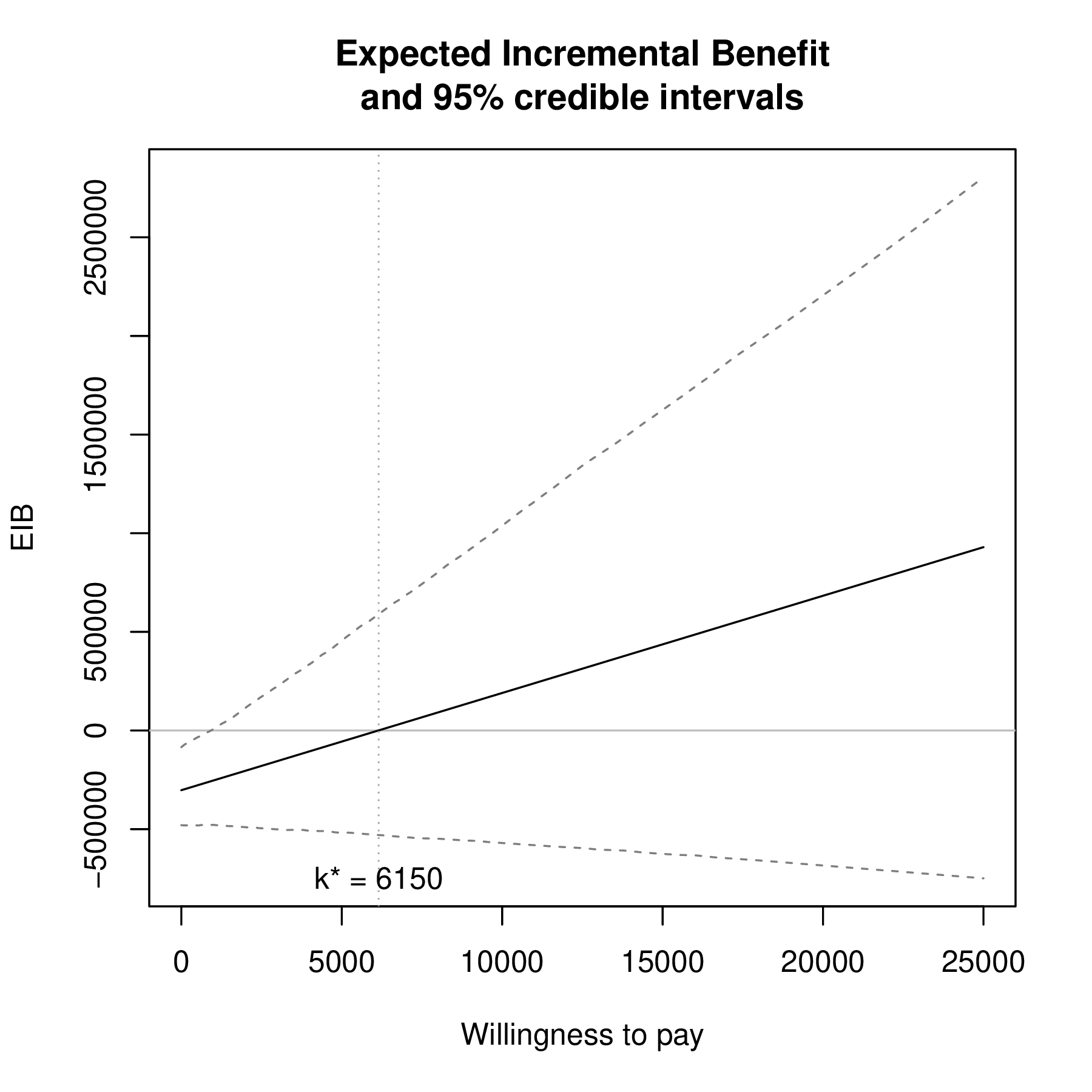
ICER vs EIB
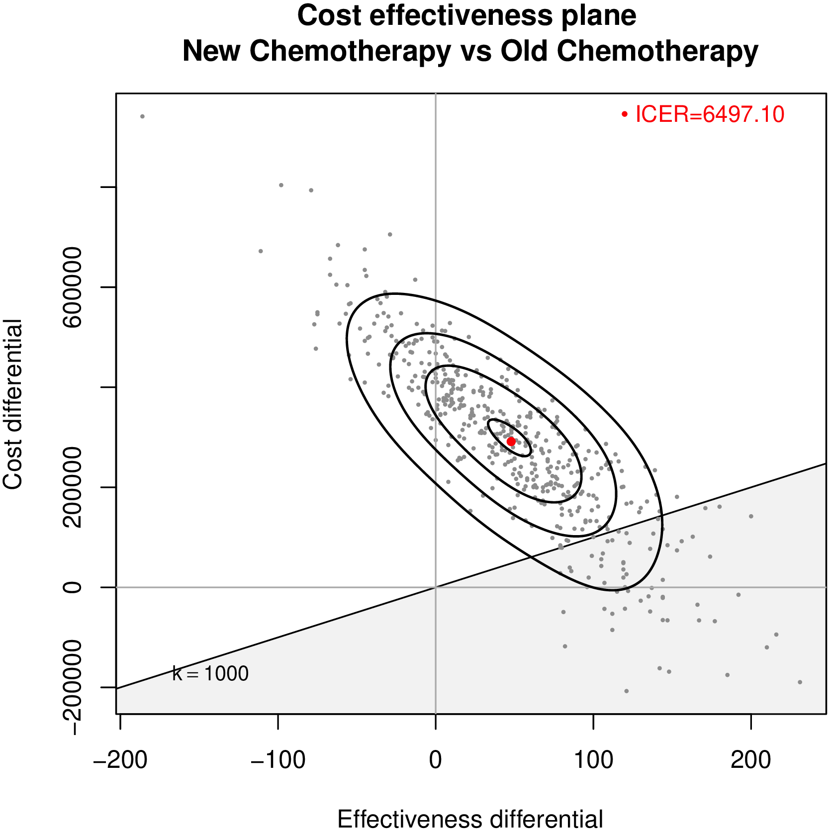
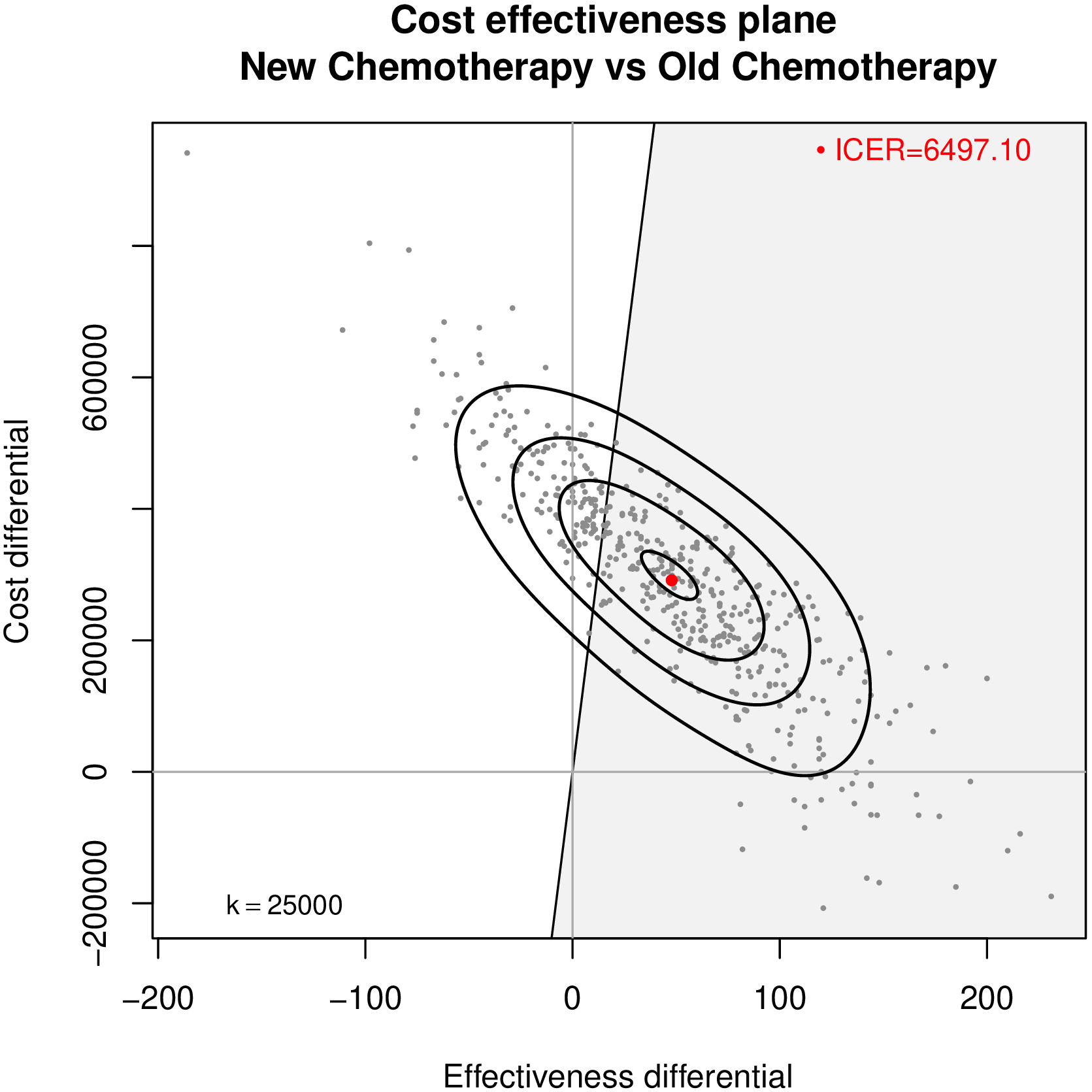
ICER vs EIB
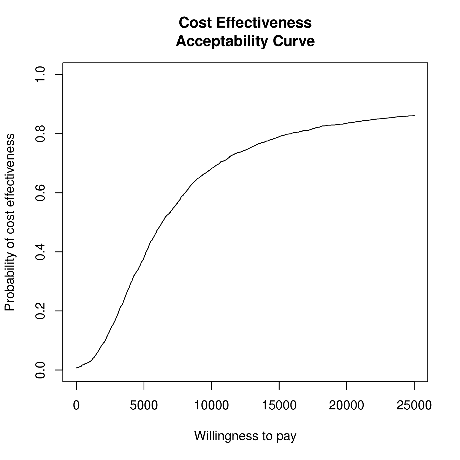
CE plane vs CEAC
CE plane vs CEAC