Statistical testing is a process aimed at using statistical modelling and the available evidence to falsify claims about an alleged data generating process (DGP); a typical example is to assume a working hypothesis that in a comparison between two interventions the true population difference in effect is 0 — that is the new treatment is no better (and no worse) than the standard of care. In a nutshell, the point of statistical testing is to aim at rejecting this hypothesis (which corresponds to a specific DGP). Medical research is probably one of the research areas in which testing has historically played a pivotal role, e.g. in the design and conduct of clinical trials, as we will see later.
Arguably statistical testing can be seen as central to the Frequentist and the Likelihood paradigm. In fact, some of the major arguments between Neyman (especially) and Pearson on the one hand and Fisher on the other hand have centered around the philophy underlying the testing procedures. As for the Bayesian approach, while suitable theory and methodology exists (which we only briefly mention in Section 4.1), it is perhaps less central to the overall paradigm. One of the reasons for this is that, by its own nature, the Bayesian analysis allows direct probabilistic statements on all the unknown features of the DGP.
Confusion
If you found the distinction between the three main schools of statistical thought discussed in the context of estimation confusing, things are even more subtly complex in terms of testing. The philosophy underlying the mathematical construction of the testing procedure is fundamentally different under the frequentist and the likelihood approach, as we will discuss later. But too often, the two have been seemlessly conflated into a unified theory — even in the common case of design and analysis of clinical trials (Goodman 1999). For this reason, it is important to realise the main features of each approach and appreciate the intrinsic distinctions, advantages and disadvantages.
In addition, recently there has been a marked shift in the scientific community, who have started to recognise and promote estimation over testing. This has also been caused by the backlash following the so-called “reproducibility crisis” linked to the (mis-)use of \(p-\)values, which has led to a position paper (Wasserstein, Lazar, et al. 2016), discussing the potential pitfalls of practices that are too heavily focussed on testing.
4.1 Bayesian approach
We show here a very simple example of Bayesian testing, based on a real analysis performed by Pierre Simone Laplace, a French mathematician who in the late 19th century made great contributions to several scientific disciplines, including Statistics. Despite its almost artificial simplicity, this example illustrate how we can use the full posterior distribution to make probabilistic statements about underlying DGPs, effectively using inference to perform a variety of testing.
Example 4.1 (Female births in Paris) We consider here the famous data analysed by Laplace on the number of female births in Paris. In 1710, John Arbuthnot, a Scottish medical doctor with a passion for mathematics, analysed data on christening recorded in London between 1629 and 1710 to conclude that males were born at a “significantly” greater rate than females. This being somehow against the assumption of equal probability for the two sexes, he deduced that divine providence accounted for it, because males die young more often than females.
Laplace analysed similar data collected in Paris from 1745 to 1770. He observed a total of \(r=241\,945\) girls born out of a total of \(n=493\,527\) babies and was interested in estimating the probability of a female birth, \(\theta\). Laplace based his analysis on a reasonable Binomial model for the data: \(r\mid \theta \sim \mbox{Binomial}(\theta,n)\) and pragmatically assigned a Uniform distribution in \([0;1]\) to \(\theta\): \(p(\theta)=1\). This assumption is meant to encode complete lack of knowledge on the model parameter — the only thing this prior is implying is that \(\theta\)has to be between 0 and 1 (which is of course true, as it is a probability). But we are assuming that any value in this range is equally likely. Although this is perhaps a rather unrealistic assumption, it simplifies computation of the posterior distribution.
With a little of algebra, it is possible to show that in this case \(\theta\mid r,n \sim \mbox{Beta}(r+1, n-r+1)\). We can use R to quantify the posterior probability that \(\theta>0.5\) (i.e. that the true data generating process does rely on a higher chance of a newborn being a male) as
# Data: number of girls (r) out of the total births (n) # in the time interval consideredr=241945n=493527# Computes the tail area probability under the posterior distribution using # simulations from the posteriornsim=10000sims=rbeta(n=nsim,shape1=r+1,shape2=n-r+1)# Tail-area probabilitysum(sims>=0.5)/nsim
[1] 0
So, given the model assumptions and the observed data, the working hypothesis that \(\theta\geq 0.5\) has essentially no support whatsoever. Laplace calculated analytically that \(\Pr(\theta\geq 0.5\mid r,n)=1.15\times 10^{-42}\) and thus concluded that he was “morally certain” that it was in fact less than 0.5, in accordance with Arbuthnot’s finding.
Bayes Factors and the strength of the evidence
Bayesian testing can get much more complicated than shown here. In principle, the main idea is to enumerate an exhaustive list of competing DGPs, indexed by a specific distributional assumption for the parameters \(\boldsymbol\theta\). For example, we may consider \(p(\theta\mid \mathcal{M}_1) \sim \mbox{Beta}(3,22)\); \(p\left(\log\left(\frac{\theta}{1-\theta}\right)\mid \mathcal{M}_2\right) \sim \mbox{Normal}(0,10)\); \(p(\theta \mid \mathcal{M}_3) \sim \mbox{Uniform}(0,1), \ldots\) — notice that for \(\mathcal{M}_2\), we are specifying a prior on a different scale (technically, this is the logit transformation, which we will see in Chapter 5).
Each of these generative models \(\mathcal{M}_1,\ldots,\mathcal{M}_K\) can be associated with a prior distribution \(p(\mathcal{M}_k)\), for \(k=1,\ldots,K\). Bayesian updating can be then applied given the data to obtain an estimate of the posterior distribution for each of the hypotheses being analyses, \(p(\mathcal{M}_k \mid \boldsymbol y)\).
Once the posterior distributions are available, we can compute the Bayes factor for model \(k\) versus model \(j\) (for \(k,j=1,\ldots,K\)) as \[\begin{eqnarray*}
\mbox{BF}_{kj} & = & \frac{p(\boldsymbol y \mid \mathcal{M}_k)}{p(\boldsymbol y \mid \mathcal{M}_j)} \\
& = & \frac{\int p(\theta\mid \mathcal{M}_k) p(\boldsymbol y \mid \theta, \mathcal{M}_k) \rm{d}\theta}{\int p(\theta\mid \mathcal{M}_j) p(\boldsymbol y \mid \theta, \mathcal{M}_j) \rm{d}\theta}
\end{eqnarray*}\]
A rule of thumb to interpret the observed value of the BF is provided by Jeffreys who suggested the following interpretation.
BF \(\in [1;3.2)\): the strength of the evidence for \(\mathcal{M}_k\) against \(\mathcal{M}_j\) is “not worth more than a bare mention”;
BF \(\in [3.2;10)\) the strength of the evidence for \(\mathcal{M}_k\) against \(\mathcal{M}_j\) is “substantial”;
BF \(\in [10;32)\) the strength of the evidence for \(\mathcal{M}_k\) against \(\mathcal{M}_j\) is “strong”;
BF \(\in [32;100]\) the strength of the evidence for \(\mathcal{M}_k\) against \(\mathcal{M}_j\) is “very strong”;
BF\(>100\) the strength of the evidence for \(\mathcal{M}_k\) against \(\mathcal{M}_j\) is “decisive”.
In reality, the computation for the BF is complicated for two reasons:
In order to derive the marginal distribution of the data given the postulated model, we need to integrate out the uncertainty about \(\theta\), described by the posterior distribution. This is essentially akin to computing some weighted average of the full models for the observed data (as a function of the prior for the models as well as the priors for the parameters within each model). As shown in the equation, this involves the computation of generally very complex integrals, thus making this calculations hard to perform.
Even if we could easily make this computation, the underlying assumption here is that we are able to enumerate all the competing DGPs. And that one of the models described by \(\mathcal{M}_1,\ldots,\mathcal{M}_K\) is indeed the truth — which we have no real means of ensuring.
Bayesian testing remains one of the most complex parts of the whole approach. And, as mentioned above, it is perhaps fair to say that, by nature, the Bayesian approach is more focused on a purely estimation context, given that the output of the posterior distribution can indeed be used to make direct probabilistic statments, as in Example 4.1. More details can be found for example in Spiegelhalter, Abrams, and Myles (2004), Gelman et al. (2013) and Kruschke (2014).
4.2 Likelihood approach: “significance testing”
Fisher’s approach to testing could arguably be seen as an extension to his estimation procedure, based on the likelihood function (you will see this extensively in both STAT0015 and STAT0016). The most basic structure of the problem is to consider a working hypothesis that represents some putative data generating process. Typically, this is some kind of “null” model, implying for instance that there is no meaningful difference in the effect of two competing interventions being tested. We call this the null hypothesis and we indicate it as \(H_0\).
For example we may consider a “two-sample problems”, where we randomise \(n_0\) individuals to intervention 0 (say, standard of care) and \(n_1\) individuals to intervention 1 (say, an innovative drug). This is a very common set up and you will encounter it repeatedly in STAT0015, STAT0016 and, to some extent, in STAT0019 too.
The total number of individuals in the study is \(n=n_0+n_1\). The data comprise of the two variables \(\boldsymbol{y}_0=(y_{10},\ldots,y_{n_{0}0})\) and \(\boldsymbol{y}_{1}=(y_{11},\ldots,y_{n_{1}1})\), where the subscript “\(10\)” indicates the first individual in the the “null” intervention arm (i.e. standard of care), while the subscript “\(11\)” indicates the first individual in the active intervention arm (the new drug). We could label our data more compactly using the notation \(y_{ij}\), where \(j=0,1\) indexes the treatment arm and \(i=1,\ldots,n_j\) indexes the individuals in each.
If the outcome is some continuous, symmetric quantity, we may be willing to describe the sampling variability in the two samples as \[ y_{10},\ldots,y_{n_{0}0}\stackrel{iid}{\sim}\mbox{Normal}(\mu_0,\sigma^2_0) \qquad \mbox{ and } \qquad y_{11},\ldots,y_{n_{1}1}\stackrel{iid}{\sim}\mbox{Normal}(\mu_1,\sigma^2_1),\] In a case such as this, we may specify the null hypothesis as \(H_0: \mu_1=\mu_0\), or alternatively (and equivalently!) \(H_0: \delta=\mu_1-\mu_0=0\) — i.e. that there is “no treatment effect” at the population level.
Given the sample data, we can produce estimates for the main model parameters. For example, as shown in Chapter 3, the MLE for \(\mu_j\) is the sample mean \(\bar{Y}_j = \displaystyle \sum_{i=1}^{n_j}\frac{Y_{ij}}{n_j}\), with observed value \(\bar{y}_j\). Using the results shown in Equation 3.11, we can prove that \[\begin{eqnarray*}
\bar{Y}_j = \displaystyle \sum_{i=1}^{n_j}\frac{Y_{ij}}{n_j} \sim \mbox{Normal}\left(\mu_j, \frac{\sigma^2_j}{n_j}\right).
\end{eqnarray*}\] Moreover, taking advantage of the mathematical properties of the Normal distribution, we can prove that if \(X_1\sim\mbox{Normal}(\mu_1,\sigma^2_1)\) and \(X_2\sim\mbox{Normal}(\mu_2,\sigma^2_2)\)independently, then
Thus, we can construct an estimator for the difference in the treatment effect \(\hat\delta=D=\bar{Y}_1-\bar{Y}_0\) and derive that \[\begin{eqnarray*}
D = \bar{Y}_1-\bar{Y}_0 & \sim & \mbox{Normal}\left(\mu_D,\sigma^2_D\right) \\
& \sim & \mbox{Normal}\left( \mu_1-\mu_0, \frac{\sigma^2_0}{n_0}+\frac{\sigma^2_1}{n_1} \right)
\end{eqnarray*}\]
If we knew the underlying values for the two population variances \((\sigma^2_0,\sigma^2_1)\), then we could use Equation 3.4 and derive that \[
\frac{D-\delta}{\sqrt{\frac{\sigma^2_0}{n_0}+\frac{\sigma^2_1}{n_1}}} \sim \mbox{Normal}(0,1).
\tag{4.1}\]
Obviously, we are not likely to have this information and thus we can first provide an estimate of \(\sigma^2_D\) using the sample variance \[\begin{eqnarray*}
S^2_D& = &\frac{S^2_0}{n_0}+\frac{S^2_1}{n_1} \\
& = & \frac{n_0}{n_0-1}\sum_{i=1}^{n_0} (Y_{i0}-\bar{Y}_0)^2 + \frac{n_1}{n_1-1}\sum_{i=1}^{n_1} (Y_{i1}-\bar{Y}_1)^2
\end{eqnarray*}\] expanding on the result shown in Equation 3.14 and then derive \[
T=\frac{D-\delta}{\sqrt{S^2_D}} \sim \mbox{t}(0,1,n-1),
\tag{4.2}\] adapting the result shown in Equation 3.15.
Fisher’s idea on testing is that we can actually use this result to compute some measure of how much support the observed data give to the null hypothesis (in this case that \(\delta=0\)).
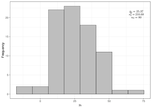
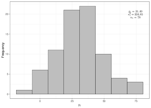
For instance, suppose that the data observed are as described by the histograms and summary statistics shown in Figure 4.1.
(a) Histogram of the sample data \(\boldsymbol{y}_0\)
(b) Histogram of the sample data \(\boldsymbol{y}_1\)
Figure 4.1: Graphical summary of the observed data
Given the sample values and estimates \[\begin{eqnarray*}
n_0 = 80; & \qquad & n_1 = 78; \\
\bar{y}_0 = 25.37; & \qquad & \bar{y}_1 = 31.40; \\
S^2_0 = 210.68; & \qquad & S^2_1 = 334.85,
\end{eqnarray*}\] we can compute the observed value for the estimate of the true difference in the two means \(d=6.02\) and the estimate for its variance \[\begin{eqnarray*}
s^2_D = \frac{s^2_0}{n_0} + \frac{s^2_1}{n_1} & = & \frac{210.68}{80} + \frac{334.85}{78} \\
& = & 2.63 + 4.29 = 6.93.
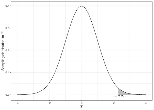
\end{eqnarray*}\]Under the null hypothesis, the observed test statistic is \[ t = \frac{d-0}{\sqrt{s^2_D}} = \frac{6.02}{2.63} = 2.29. \]
Fisher thought that if the null hypothesis were true, then we would expect the observed value \(t\) of the test statistic \(T\) to be fairly “central” in the range of its sampling distribution. In other words, he suggested using tail-area probabilities under the sampling distribution \(p(t\mid\theta,H_0)\) to find the chance of observing a result “as extreme as, or even more extreme than” the one that actually obtained in the current data. Intuitively, if \(t>\mbox{Med}(T)\), i.e. the observed value of \(t\) is “larger than normal”, we would be looking at even larger values; conversely, if \(t\leq \mbox{Med}(T)\), “even more extreme” values would be in fact smaller than that observed.
In the present case, we can use R to compute the \(p-\)value\(\Pr(T>t\mid \theta,H_0)\)
# Computes the tail-area probability under the sampling distribution under H_0# NB: the option 'lower.tail=FALSE' computes the area to the *right* of the# observed value tpt(q=t,df=n-1,lower.tail=FALSE)
[1] 0.01170658
They didn’t have a computer…
Equation 4.1 and Equation 4.2 construct the relevant test statstics using a re-scaling of the quantity of interest \(D\). This is essentially a historical accident — the reason for this is that even if we could determine that \(D\) was associated with a Normal sampling distribution, in practical terms, without computers it was difficult (although not impossible) to compute probabilities for a non-standard Normal (i.e. one with mean different than 0 and variance different than 1). Conversely, computations with a standard Normal (or, for that matter, with a t with mean equal to 0 and variance equal to 1) are much simpler to perform by hand, which Fisher had pretty much to do. With modern computers, we do not really worry about re-scaling the relevant quantity \(D\) to the standardised test statistics \(Z\) and \(T\). But because re-scaling does not really cost much in computation terms (in fact, hardly anything at all!), this procedure has stuck and we still use it.
The \(p-\)value is the area shaded to the right of the observed \(t=2.29\), in Figure 4.2 (note that the value of \(t\) is greater than the median of the distribution and so we need to look for the tail-area in the right). Because the probability of observing something as extreme as, or even more extreme than the data we have actually got in front of us is extremely small, we deem that the data provide very little support to the working hypothesis of no difference in the population means.
Figure 4.2: The sampling distribution for the statistic \(T\). The shaded area indicates the \(p-\)value
p-values and continuous distributions
The interpretation of the \(p-\)value in terms of assessing the probability of observing something as extreme as, or even more extreme than the data actually observed (or, in other words, as a tail-area probability) is clearly a mouthful and a slightly subtle concept.
The reason why Fisher had to use such a convoluted phrasing is that, when dealing with continuous data, the sampling distribution does not really represent a probability, but rather a density. So, it is impossible to quantify the strength of the evidence just in correspondence of the observed value for the test statistic.
One criticism associated with this (inevitable!) choice is that the strength of the evidence (or, in other words: whether the observed data are consistent with the working hypothesis) depends on the data actually observed, as well as on data (“even more extreme”) that might be — but have not been — observed.
In addition to this, by its own nature, it is possible that the same \(p-\)value is computed for a very small and a very large study; the conclusion in terms of strength of the evidence would be identical, without distinction of the underlying sample size (Goodman 1999).
In a similar way to Jeffreys, Fisher also provided some rule of thumb to interpret the \(p-\)value \(P\) observed from the data at hand.
If \(P<0.01\), then conclude that there is strong evidence against \(H_0\);
If \(0.01<P<0.05\), then conclude that there is fairly strong evidence against \(H_0\);
If \(P>0.05\), then conclude that the there is little or no evidence against \(H_0\), or alternatively, that the observed data are consistent with the model specified in \(H_0\).
Of course, there is nothing special about the value 0.05 (5%), which is effectively used as the threshold for statistical significance. And more importantly, can a dataset giving rise to a \(p-\)value of 0.0499 really be considered as substantially different than one giving rise to a \(p-\)value of 0.0501? Yet, for a very long time, medical and psychology journals in particular have obsessed over the “quest for significance”, at times refusing to publish studies with results indicating a \(p-\)value above 0.05 as irrelevant.
Confidence intervals and p-values
Suppose we test a null hypothesis \(H_0: \mu = \mu_0\) and find that the \(p-\)value is greater than 0.05. Then the 95% confidence interval for \(\mu\) will include the hypothesised value \(\mu_0\). If \(P < 0.05\) then the 95% confidence interval will not include \(\mu_0\). In other words:
The 95% confidence interval for \(\mu\) consists of all hypothesised values \(\mu_0\) for which the \(p-\)value is greater than 0.05.
Thus, if you calculate a 95% confidence interval that does not include a \(\mu_0\) of interest, then you can infer that the \(p-\)value will be less than 0.05. Likewise, if a 99% confidence interval does not include \(\mu_0\), the \(p-\)value will be less than 0.01. Note, though, that there is a logical disctinction between estimation and testing.
4.3 Frequentist approach: “hypothesis testing”
The main idea underlying Neyman and Pearson’s (NP’s) approach to testing is that, in fact, this is not an inferential problem, but rather a decision-making one.
The rationale in NP’s approach is that the researcher does not really believe in \(H_0\) — if we thought that a new drug did not really have any difference over something that already exists, what would be the point in investing money, time and research in developing it? \(H_0\) is just a working hypothesis that we would like to discard, or in technical parlance reject, given the observed data (and the modelling assumptions we are making!).
For instance, what the researchers would probably truly believe is that in fact intervention 1 is more effective than intervention 2 (i.e., assuming that the higher the population mean, the better the health condition, that \(\mu_1>\mu_0\)). Thus, we can also specify an alternative hypothesis\(H_1: \mu_1>\mu_0\) or, equivalentely \(H_1:\delta>0\), to indicate that the new intervention is better.
Unlikely events
One important and perhaps subtle feature of the testing procedure is the distinction between the idealised (null) hypothesis and the empirical evidence we want to use to disprove it.
The null and the alternative hypotheses are defined in terms of the population parameters. So by considering \(H_0:\mu_1=\mu_0\) we are assuming that the “true” average intervention effects are identical.
However, we will never be in a position of osserving the population parameters. All we can do is get some sample data and then use suitable statistics to estimate the underlying parameters and then say something about whether these are equal or not. So it is perfectly possible that, just by chance, we observe data that look like they could be drawn by a common generating process where the two population means are the same. But in fact the underlying, true DGP may be characterised by different means (perhaps where the difference is only little).
For this reason, NP have framed their hypothesis testing problem in terms of the decision made about whether or not the null hypothesis is the underlying truth, based on the current data. Table 4.1 shows this schematically (and you will see more on this in STAT0015 and STAT0016).
Table 4.1: The decision problem underlying NP’s theory of hyphotesis testing
$H_0$ true
$H_0$ false
Reject $H_0$
Type I error $\alpha$ (False positive)
Correct inference (True negative)
Fail to reject $H_0$
Correct inference (True positive)
Type II error $\beta$ (False negative)
If the true “state of nature” was that there is in fact no difference in the intervention effects (labelled as “\(H_0\) true”), if the data make us reject\(H_0\), then we would be making an error. NP call this “Type I error”, indicated as \(\alpha\) — this is essentially a “false positive”, because we would be erroneously claiming that there is a difference in the intervention effects, when in fact there is not. Conversely, if the data make us fail to reject \(H_0\), then we would be making the correct decision. The Type I error is also usually (and rather confusingly!) referred to as “significance level”.
Similarly, if the true “state of nature” was that the new intervention is more effective (i.e. there is a difference in the population means), then the situation is reversed: if we have enough evidence to reject the null hypothesis, then we would have made the correct decision. But if the data were not indicating that we should reject \(H_0\), then we would be making an error. NP call this the “Type II error” \(\beta\), which can be thought of as a “false negative” result, because we would conclude that there is no difference, when in fact one is present.
In particular, in a typically frequentist fashion, we can reason along the following lines: if we were able to replicate the experiment (data collection) over and over again, under the same experimental conditions we would have the following situation.
If \(H_0\) is indeed the true DGP, then we would make the wrong decision in a proportion of times equal to \(\alpha\), while we would make the correct decision in the complementary proportion of times \(1-\alpha\).
If \(H_1\) is indeed the true DGP, then we would make the wrong decision in a proportion of times equal to \(\beta\), while we would make the correct decision in the complementary proportion of times \(1-\beta\).
The researcher is given the choice to tune the two unknown probabilities: NP’s suggestion (which has essentially become some kind of dogma in many areas of applied research) is that it is good to keep the probability of making a Type I error \(\alpha\) to a very low value, typically 1 in 20, or 0.05. This means that if we were able to do the experiment a very large number of times under the same conditions if \(H_0\) is the true state of nature, on average we would correctly fail to reject the null hypothesis 95% of the times (approximately 1 every 20 replicates).
As for the Type II error, NP suggested that, somewhat arbitrarily, the researcher could live with a less stringent requirement and typically \(\beta\) is fixed at either 10% or 20%. This means that if there truly is an intervention effect (i.e. \(H_1\) is the “truth” and thus the two population means are different), we are happy to mistakenly claim the opposite result in 10-20% of the times. Intuitively, the rationale for this imbalance in the values of \(\alpha\) and \(\beta\), can be explained as follows. Most likely, the “status quo” intervention (with population mean \(\mu_0\)) will be established and probably a “safe option”. The new intervention may be very good and improve health by a large amount. But of course we are not sure, because perhaps the data are limited in scope and follow up. Thus, we want to safeguard against making claims that are too enthusiastic about the potential benefits of the new intervention — that is why we keep the Type I error probability to a low value. Conversely, although it is bad to miss out on claiming that the new intervention is in fact beneficial, we are more prepared to run this risk — and that is why \(\beta\) is typically higher than \(\alpha\).
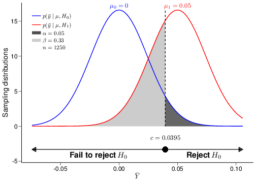
The graph in Figure 4.3 visualises the ideas underlying the procedure for hypothesis testing. For the sake of argument, imagine that the true DGP is characterised by a Normal distribution where the population mean and variance are \(\mu=0.01\) and \(\sigma^2=0.85^2\).
Figure 4.3: A graphical depiction of the decision-making problem in hypothesis testing
For simplicity (and unrealistically!), we assume that we, the researchers performing the analysis, do know the true value of the population variance, while the population mean is unknown to us. We then define the null hypothesis as \(H_0: \mu=\mu_0=0\) in contrast with the alternative \(H_1: \mu=\mu_1=0.05\). As is almost invariably the case, the alternative hypothesis does not represent the “truth”, but simply a proposed model in which the treatment does have a (clinically meaningful) effect — and in this particular case, the true treatment effect \(\mu\) happens to be closer to \(H_0\) than it is to our posited alternative DGP, indexed by \(H_1\). Also, we assume that data are observed for \(n=1250\) individuals and these are modelled as \(y_1,\ldots,y_n\stackrel{iid}{\sim}\mbox{Normal}(\mu,\sigma)\).
Suppose that we decide to consider as test statistic the sample mean \(\bar{Y}\). Given the model assumptions specified above and recalling Equation 3.11, we know that \[
\displaystyle \bar{Y}\sim\mbox{Normal}\left(\mu=0.01,\frac{\sigma}{\sqrt{n}}=\frac{0.85}{35.36}=0.024\right)
\tag{4.3}\] (of course, in reality, we would not know the true values for the parameters, but remember that in this example, we are pretending to be some kind of Mother Nature figure, who knows all…).
By plugging in the values for the hypothesised means \(\mu_0\) and \(\mu_1\), we can derive the sampling distributions under the two competing hypotheses \[\displaystyle p(\bar{y}\mid \theta,H_0)=\mbox{Normal}\left(0,0.024\right) \qquad \mbox{ and } \qquad \displaystyle p(\bar{y}\mid \theta,H_1)=\mbox{Normal}\left(0.05,0.024\right).\] Notice that, unlike the model in Equation 4.3, even without the gift of being Mother Nature, we are in general able to determine these two distributions, because they depend directly on our model assumptions and the observed data, which allow us to estimate the relevant parameters.
The two sampling distributions are shown in Figure 4.3 as the blue and red curve, respectively. The dark grey area under the blue curve represents the tail-area probability under the null sampling distribution, which we have constructed to be equal to \(\alpha\). Similarly, the light grey area under the red curve represents the tail-area probability under the alternative sampling distribution, equal to \(\beta\) (\(=0.33\), given the model assumptions specified in this case).
The 95% quantile of the sampling distribution under \(H_0\), computed as \(c=0.0395\) in the present case, is indicated as the large dot above the \(x-\)axis in Figure 4.3. NP refer to this as the “critical value”, because it determines the “critical” (or “rejection”) region: if the observed value of the test statistic determined by the data lies in the rejection region, then the data give more support to the sampling distribution under \(H_1\). Intuitively, we can see this by considering that for each point in the region labelled as “Reject \(H_0\)” in Figure 4.3 (i.e. the dark grey area), the density is higher under the red, than under the blue curve. If, on the contrary, the observed value of the test statistic does not lie in the rejection region (i.e., in this case is less than the critical value), then we do not have enough evidence to reject the null hypothesis. This is the decision rule underpinning the procedure of hypothesis testing:
If the observed value of the test statistic is in the critical region (which is determined by the model assumptions and the observed data), then reject \(H_0\). If not, we fail to reject \(H_0\).
Fisher vs Neyman-Pearson
Superficially, Fisher’s procedure of significance testing and NP’s hypothesis testing, look rather similar. They both depend on defining some null hypothesis (typically indicating the lack of treatment effect, i.e. meaningful difference between two mean responses), which we do not really believe in but would like to be able to falsify; then they both involve the definition of some test statistic, for which we could determine a sampling distribution, based on the model assumptions; then they both involve computing the value of the test statistic.
Where they differ (substantially!) however, is that significance testing outputs a \(p-\)value, which is a numerical summary of the “strength of the evidence” against \(H_0\). We can make a decision based on the \(p-\)value, as outlined above — so if it is very small, we can safely reject \(H_0\), while if it is borderline the set significance level (e.g. 0.05), our assessment will be much less certain.
On the contrary, NP’s procedure has a strictly binary outcome: whether the observed value of the test statistic falls just above the critical value, or it is much, much larger, it is actually irrelevant for the decision problem: in both cases, we would reject \(H_0\).
These two interpretations are often conflated — and \(p-\)values tend to be evaluated under this strict binary decision rule.
Another important distinction between signficance and hypothesis testing is that in the former case, we do not take explicit notice of the alternative DGP described by \(H_1\), which is a central part to NP’s theory. The main advantage of the fact that we do consider an alternative mechanism to generate the data is that, given the significance level \(\alpha\) and the sample size of the dataset we wish to use to compute the test statistic, we can also assess the chance of making a Type II error, which we have indicated as \(\beta\), above. For example, for \(\alpha=0.05\) and \(n=1250\) as shown in Figure 4.3, the resulting Type II error is \(\beta=0.33\). This automatically allows us to compute the “power” of the test statistic, \(1-\beta\), which indicates the probability of rejecting \(H_0\), when it is false.
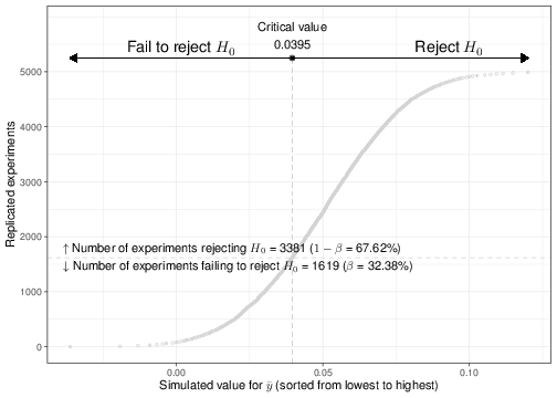
We can use a simulation approach to better understand this concept. Given the model assumptions above, we can use R to simulate a large number of potential replicates of the experiment (i.e. the data collection), assuming that \(H_0\) is false. For example, we could use the code below.
Figure 4.4: Output of 5000 simulations for data of sample size \(n=1250\), generated from \(H_1\)
Figure 4.4 shows a graphical summary of the results for this simulation, when we use a sample size of \(n=1250\) and consider \(n_{\rm{sims}}=5000\) replicates. The \(x-\)axis indexes the value of the simulated test statistic \(\bar{Y}\) that is obtained for each replicate of the experiment — for better visualisation, these have been sorted from the lowest (-0.036) to the highest value (0.15). Each dot in the plot is the computed value of \(\bar{Y}\). The dashed vertical line indicates the critical value \(c=0.0395\), which in turns determines the rejection region.
As is possible to see, when we set \(\alpha=0.05\) and \(n=1250\), the percentage of simulations for which we correctly manage to reject \(H_0\) (remember that we are simulating data from the alleged DGP under \(H_1\), which means that \(H_0\)is false!) is about 68%, in line with the theoretical outcome shown in Figure 4.3.
Likelihood ratio tests
As is customary within the frequentist approach, the choice of a possible test statistic depends on a set of long-run properties that define its optimality. There are of course very many potential choices that can be made — the discussion of these properties is beyond the scope of these notes.
In many practical cases, it can be proved that among all tests for a specified level \(\alpha\) and for a set sample size \(n\), the likelihood ratio test statistic, defined as \[\begin{eqnarray*}
\Lambda(\boldsymbol{Y}) = \frac{\mathcal{L}(\theta\mid \boldsymbol{Y},H_0)}{\mathcal{L}(\theta\mid \boldsymbol{Y},H_1)}
\end{eqnarray*}\] is the one with the highest power and this is often regarded as an optimal property, thus justifying the use of this test statistic in many applied cases. Intuitively, the likelihood ratio is small if the alternative model is better than the null model.
In particular, it can be proved that, at least approximately, \[ -2\log\Lambda(\boldsymbol{Y}) \sim \mbox{Chi-squared}(\nu), \] where the degrees of freedom are determined by the type of the hypotheses being tested.
If we define \(\chi_{(1-\alpha)}(\nu)\) as the \(100(1-\alpha)\%\) quantile of the Chi-squared\((\nu)\) distribution, then the (2-log)likelihood-ratio test provides the decision rule as follows:
If \(-2\log\Lambda(\boldsymbol{Y})>\chi_{(1-\alpha)}(\nu)\), then reject \(H_0\)
If \(-2\log\Lambda(\boldsymbol{Y})\leq\chi_{(1-\alpha)}(\nu)\), then fail to reject \(H_0\).
More details can be found for example in Casella and Berger (2002).
Because of the obvious relationship between the sample size \(n\) and the level of precision with which we can estimate the model parameters, which essentially determines the variance of the observed data \(\boldsymbol{Y}\) and therefore of the test statistic \(f(\boldsymbol{Y})\), we can then use the power for two important purposes:
As a tool to determine the “best” test, for a given significance level and set sample size.
As a tool to determine the “optimal” sample size we need to observe to be able to constrain the Type II error, given a fixed significance level.
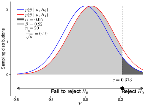
(a) \(n=20\)
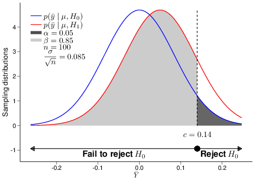
(b) \(n=100\)
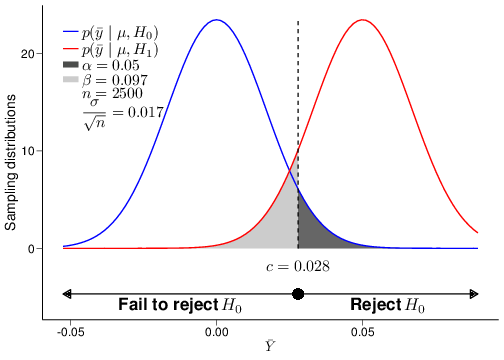
(c) \(n=2500\)
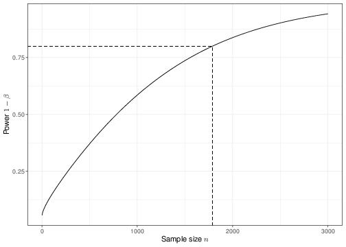
(d) Power function
Figure 4.5: The relationship between power and sample size
Figure 4.5 shows an example of the analysis shown above for several choices of the underlying sample size, in this case \(n=20,100\) and \(2500\). As is possible to see, the standard deviation for the sampling distribution of the test statistic \(\bar{Y}\), which in this case is given by \(\frac{\sigma}{\sqrt{n}}\), does decrease for increasingly large values of the sample size \(n\). This implies that a different critical value \(c\) would be computed in each of the three cases depicted in panels (a)—(c).
When the sample size is very small, then the two sampling distributions under \(H_0\) and \(H_1\) are very close together, because the means \(\mu_0\) and \(\mu_1\) are also assumed to be fairly close and the standard deviation is relatively large. Intuitively, this means that it will be difficult to tell them apart, which in turns means that we are very much prone to mistakes in the decision-making (and so we would fail to correctly reject \(H_0\) a large proportion of times — in fact about 92% of the times). Thus, for such a small sample size, the power is very low.
But when we increase the sample size, we also tend to increase the power of the test, i.e. its ability to correctly detect a signal, while keeping fixed its ability to safeguard from claiming a false significant results. By plotting the power resulting for a range of possible sample sizes, we get the graph in panel (d), which is often referred to as the power function of the test.
At the stage of designing a study, we could use the power function to determine the sample size that is necessary so that the resulting test has a significance level (i.e. Type I error) \(\alpha\) and a power \(1-\beta\), for fixed values of \(\alpha\) (i.e. almost invariably 0.05) and \(\beta\) (e.g. 0.2). In the current case, given all the model assumptions, we would need to observe at least \(n=1787\) individuals to be able to detect a difference of \(\mu_1-\mu_0=0.05\) with 80% power — this is indicated by the vertical dashed line in panel (d) of Figure 4.5.
\(\alpha\) vs \(P\)
The sample size calculation, or power analysis, shown above highlights another subtle idiosyncrasy of the “combined” Fisher/NP approach (which, as we have mentioned above, neither of the original proponents would have condoned!). Medical research is designed according to NP’s precepts, which aim at controlling the Type I and II errors by setting a fixed signficance level \(\alpha=0.05\) and then optimising the sample size \(n\) in order to obtain a power of \(1-\beta\) (typically 0.8). But then, once the data are actually collected, the analysis is performed under a Fisherian approach, which is based on the calculation of the \(p-\)value.
And despite the fact that the common threshold value for both \(\alpha\) and \(P\) are usually set at 0.05, these are two fundamentally different quantities: \(\alpha\) is set from the outset and it is immutable and independent on the data that are actually observed. \(P\), on the other hand, is determined by the actual data and is meant to provide a graded measure of the strength of the evidence against the null hypothesis (and, notably, without any formal regards to what is the alternative hypothesis).
4.4 Commonly used statistical tests
In this section, we present some of the most common statistical tests (with specific reference to the Likelihood approach and the use of \(p-\)value). You will see these in many of the different topics discussed in STAT0015 and STAT0016.
4.4.1 Chi-squared test
The Chi-squared test is encountered in many applied cases. One of the most important cases is the comparison between groups of categorical data, e.g. grouped in a contingency table such as the one presented below.
Table 4.2: An example of categorical data grouped by treatment arm and clinical output
Disease cured
Disease not cured
Total
Control arm
13
40
53
Treatment arm
18
29
47
Total
31
69
100
We can rescale the data in Table 4.2 to compute the probability that a random patient is cured from the disease under the two treatment arms \(\displaystyle p_C=\frac{13}{53}=0.245\) and \(\displaystyle p_T=\frac{18}{47}=0.383\). A reasonably relevant null hypothesis would be that there is in fact no association between the disease status at the end of the study period and the treatment arm.
If this null hypothesis is true, then we would expect that the total number of patients who are cured from the disease (31) would be re-proportioned in the two groups simply according to the overall sample size observed in them (i.e. 53 and 47, respectively), without any differential impact of the treatment. Thus, under \(H_0\), we would expect to see \[\displaystyle E_{CC}=53\times\frac{31}{100}=16.43\] patients who are cured from the disease in the control arm and \[\displaystyle E_{CT}=47\times\frac{31}{100}=14.57\] in the treatment arm — the notation \(E_{CC}\) and \(E_{CT}\) is meant to convey the concept of expected outcome among those \(C\)ured by the disease in the \(C\)ontrol and \(T\)reatment arm, respectively, under \(H_0\). Using a similar reasoning we can compute \[\displaystyle E_{DC}=53\times\frac{69}{100}=36.57\] and \[\displaystyle E_{DC}=47\times\frac{69}{100}=16.43,\] which indicate the expected number of patients who are still \(D\)iseased in the \(C\)ontrol or \(T\)reatment arm, respectively, under \(H_0\).
We can construct a test statistic that aims at comparing the observed data to the expected ones, under the null model as \[\begin{eqnarray*}
T = \sum_{i=(C,D)}\sum_{j=(C,T)} \frac{(Y_{ij}-E_{ij})^2}{E_{ij}},
\end{eqnarray*}\] where \(Y_{ij}\) are the values in the cells of the contingency table and for which the observed sample value is \[\begin{eqnarray*}
t & = & \frac{(13-16.43)^2}{16.43} + \frac{(40-36.57)^2}{36.57} + \frac{(18-14.57)^2}{14.57} + \frac{(29-32.43)^2}{36.57} \\
& = & 0.716 + 0.322 + 0.807 + 0.363 \\
& = & 2.21.
\end{eqnarray*}\]
Recalling Equation 2.10, we can prove that (at least approximately) \(T\sim\mbox{Chi-squared}(\nu)\), where the degrees of freedom \(\nu\) are computed as \((J-1)\times(I-1)\), where \(J\) and \(I\) are respectively the number of rows and columns in the contingency table. Thus, in this case we have that \(\nu=(2-1)\times (2-1)=1\). We can use this information to compute a \(p-\)value to measure the strength of the evidence against the null hypothesis of no association between the treatment and the probability of curing the disease as the tail-area probability under a Chi-squared distribution with 1 degree of freedom, for example using the following R commands.
# Defines the number of rows and columns of the contingency tableI=J=2# Constructs the contingency table Y=matrix(c(13,40,18,29),byrow=T,nrow=I,ncol=J)# Constructs the matrix of expected countsE=matrix(NA,J,I)for (i in1:I) {for (j in1:J) { E[j,i]=sum(Y[j,])*sum(Y[,i])/sum(Y) }}# Computes the test statistict=sum(((Y-E)^2)/E)# Computes the p-value based on the Chi-squared((J-1)(I-1)) distributionpchisq(q=t,df=((J-1)*(I-1)),lower.tail=FALSE)
[1] 0.1372945
In this case, the \(p-\)value is substantially greater than 0.05 and therefore we cannot reject the null hypothesis of no association. An alternative (more compact) way of performing the Chi-squared test is to use the built-in function chisq.test.
One vs two sided tests
As mentioned above, the \(p-\)value computed using the \(T\) statistic and the tail-area of the Chi-squared distribution does not account for what is the alternative — it is just the probability of getting something as extreme as, or even more extreme than the observed value \(t\), if \(H_0\) is true.
Often, however, available software programmes also conflate Fisher’s with NP’s interpretation and, while returning a \(p-\)value as the main output of the calculation, they will also offer the user the option to select one of three possible alternative hypotheses. For instance, there is another built-in function named prop.test that can be used to perform a Chi-squared test on proportions. This includes the option alternative that takes by default the value "two.sided", implying that the alternative hypothesis \(H_1\) assumes that the true parameter \(\theta\) simply is different than the value specified under \(H_0\), \(\theta_0\). In addition to that, prop.test also allows the user to specify the values "less" or "greater", which imply alternatives in the form \(\theta<\theta_0\) or \(\theta>\theta_0\), respectively.
This is essentially against the very nature of the \(p-\)value approach: because, to be pedantic, it is defined as the probability of getting a result as extreme as, or even more extreme than the one observed, a \(p-\)value is by definition only meant to deal with an implicitly “one-sided” alternative hypothesis. If \(t\) is “large”, then this implies that “more extreme” possible results should be measured on the right tail-area of the sampling distribution under \(H_0\). If it is “small”, then the left tail-area is to be used for the computation.
In practice, often \(p-\)values are used to report the results of a hypothesis tests, but it is important to understand that this implies some sort of hybrid methodology.
The following example clarifies the issue. Given the data in Table 4.2, we can use the R function prop.test to investigate the evidence against the null hypothesis of equality of the population proportions. This is simply done as
    2-sample test for equality of proportions without continuity correction

data:  Y
X-squared = 2.208, df = 1, p-value = 0.1373
alternative hypothesis: two.sided
95 percent confidence interval:
 -0.31861433  0.04322292
sample estimates:
   prop 1    prop 2
0.2452830 0.3829787
This configuration assumes the default implicit “two-sided” alternative (i.e. that the population proportions under the treatment and control arms are just different, without specifying a direction for this difference). The option correct=FALSE does not correct for the fact that the actual data are discrete counts, while the Chi-squared distribution is continuous (this is a technicality and only relevant when the observed counts are very small — as a rule of thumb, if there is any cell with a value less than 5, the continuity correction should be applied).
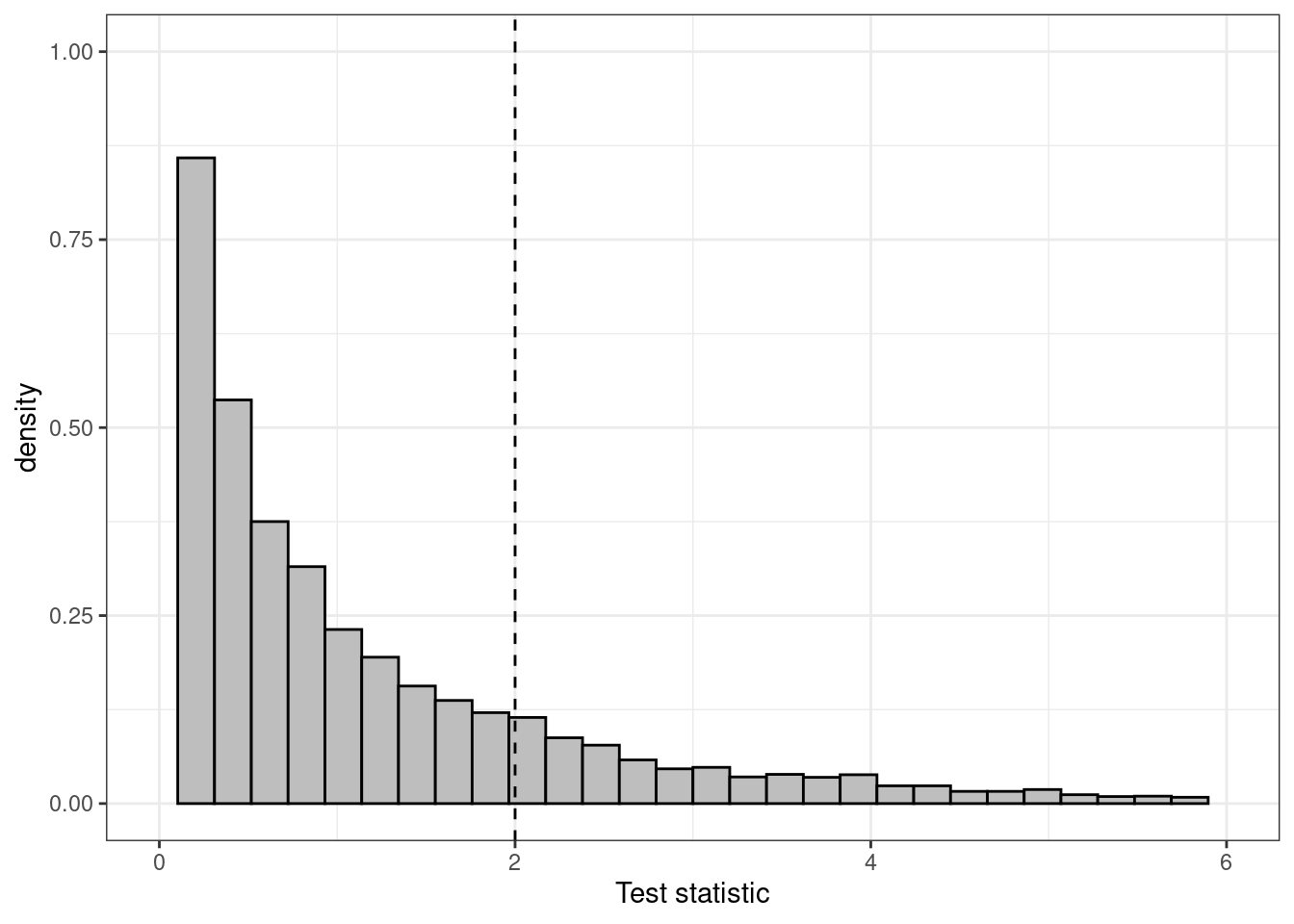
(a) Histogram for the distribution of the test statistic
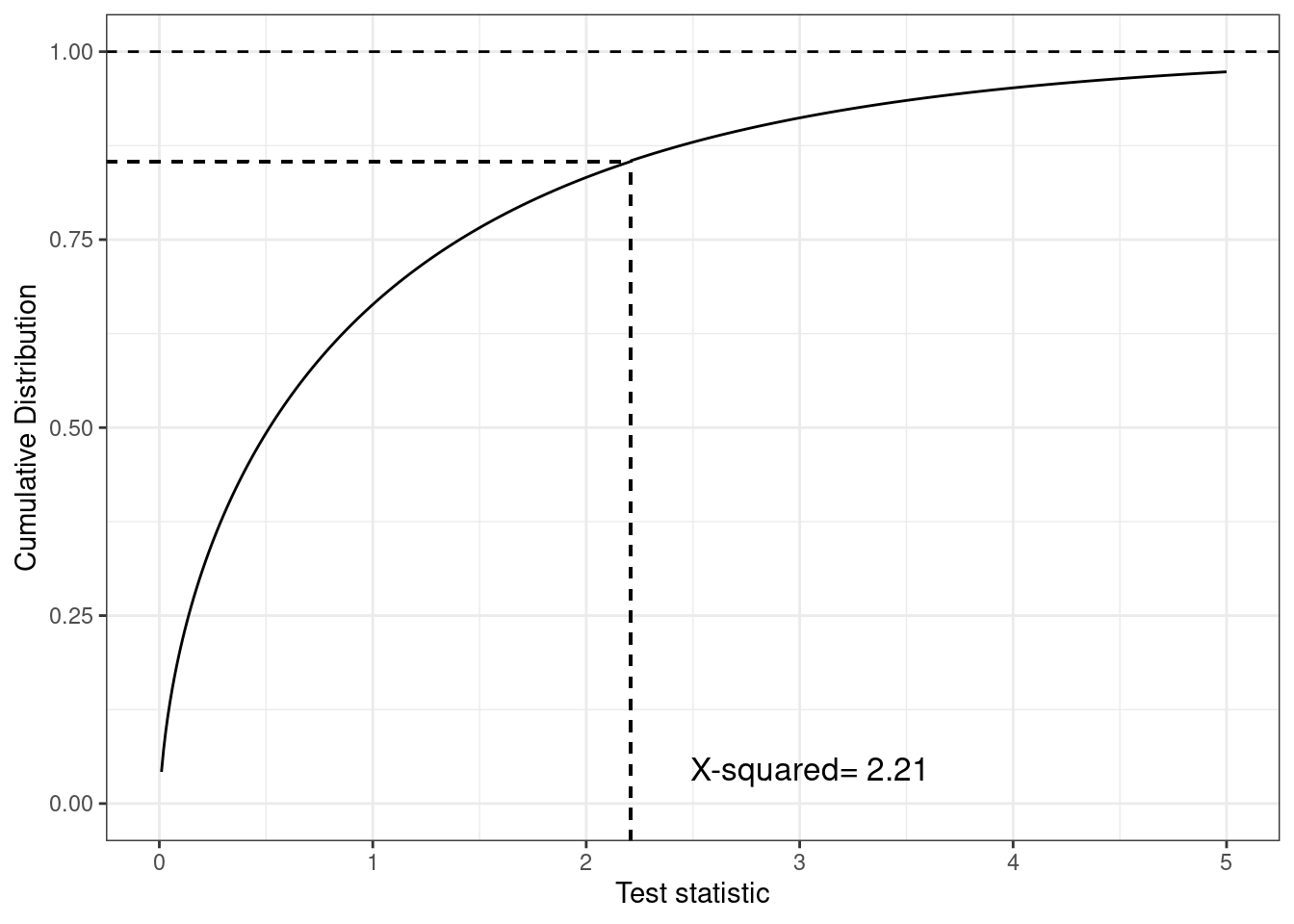
(b) Cumulative distribution of the test statistic
Figure 4.6: Different representations of the test statistic, highlighting the \(p-\)value as the tail-area probability. The histogram shows that most of the density is distributed before the observed value of the test statistic (indicated by the vertical dashed line), but the cumulative distribution plot in panel (b) highlights this more clearly
As is possible to see, this command returns the same \(p-\)value shown above, \(P_{\rm{two.side}}=0.137\), based on the same value of the test statistic (indicated as X-squared in the computer output above). The graph in Figure 4.6 shows a histogram for the distribution of the resulting test statistic in panel (a), as well as the cumulative distribution function in panel (b). This shows, for each value on the \(x-\)axis the probability that the test statistic is less than or equal to that value. So, in correspondence of the observed value 2.21, we can see that the cumulative distribution function is around \(0.863\) (i.e. the probability that the test statistic is greater than this observed value is \(1-0.863=0.137\), as reported by the computer outcome).
However, if we use the option alternative="greater", with the idea that in fact we want to consider the alternative hypothesis that the treatment arm is associated with a larger probability of being cured, we can run the command
    2-sample test for equality of proportions without continuity correction

data:  Y
X-squared = 2.208, df = 1, p-value = 0.9314
alternative hypothesis: greater
95 percent confidence interval:
 -0.2895274  1.0000000
sample estimates:
   prop 1    prop 2
0.2452830 0.3829787
and obtain a different \(p-\)value: \(P_{\rm{great}}=1-P_{\rm{two.side}}/2 = 0.931\). The rationale here is to essentially split the tail-area probability to account that when the implicit alternative hypothesis is that the parameter is different than the null value, then it may be either smaller, or greater. Assuming that these two are (at least approximately) equally likely, then we can obtain the \(p-\)value associated with the implicit alternative that the parameter is greater than the null as \(=P_{\rm{two.side}}/2 (=0.0686\) in this case).
Again, this interpretation of \(p-\)values is only possible in a combined approach where the design is based on NP’s explicit set up of null and alternative hypotheses, but the analysis is based on the graded summary of the evidence provided by the \(p-\)value, rather than the binary reject/fail to reject decision-making approach advocated by NP.
4.4.2 Fisher’s exact test
The analysis of Table 4.2 based on the Chi-squared distribution is valid but based on an approximation of the sampling distribution of the test statistic. In fact, Fisher was able to determine this distribution more precisely, by investigating the make-up of the contingency table. He was able to prove that for a generic table of counts such as the one shown in Table 4.3:
Table 4.3: A general example of a contingency table
Disease
Healthy
Total
Control
$a$
$b$
$a+b$
Treatment
$c$
$d$
$c+d$
Total
$a+c$
$b+d$
$n=a+b+c+d$
the exact distribution of the configuration of values \((a,b,c,d)\) was: \[p(a,b,c,d) =\ \displaystyle \frac{\left(\begin{array}{c} a+b \\ a\end{array}\right) \left(\begin{array}{c} c+d \\ c \end{array}\right)}{\left(\begin{array}{c} n \\ a+c \end{array}\right)} = \frac{\left(\begin{array}{c} a+b \\ b\end{array}\right) \left(\begin{array}{c} c+d \\ d \end{array}\right)}{\left(\begin{array}{c} n \\ b+d \end{array}\right)}\] (this is technically a Hypergeometric distribution). We can use this to compute an exact \(p-\)value, by enumerating all the possible configurations in which, for a fixed overall total sample size \(n\), we would observe a result as extreme as, or even more extreme than the one we have actually encountered. The difficulty in the computation is not so much in obtaining the actual probability associated with a given configuration (that Fisher proved how to compute analytically), as much as in the enumeration of all the relevant cases.
For example, for the data in Table 4.2, having fixed the margins of the table to \((53, 47)\) along the rows and \((31,69)\) along the columns, “more extreme cases” include the tables where, instead of the observed \(a\) = 13, the first cell has values \(12, 11,\ldots, 0\) (notice that by modifying the first cell of the tables implies that we also modify the second cell to respect the row margin, but also the third cell of the table so that the first column total is respected. And by doing this, we are also modifying the fourth cell of the table so that the second row total as well as the second column total are also respected).
We can make this computation using the R built-in function
fisher.test(Y)
    Fisher's Exact Test for Count Data

data:  Y
p-value = 0.1935
alternative hypothesis: true odds ratio is not equal to 1
95 percent confidence interval:
 0.2018786 1.3434546
sample estimates:
odds ratio
 0.5270614
The function outputs several results. The most important one is the \(p-\)value \(P=0.194\). This is slightly larger than the one computed using the Chi-squared test. This is a common feature of Fisher’s exact test.
Warning
Despite using the exact sampling distribution under \(H_0\) for the relevant test statistic (as opposed to an approximation based on the Chi-squared distribution), the Fisher’s exact test is often criticised as being “too conservative”, i.e. as producing \(p-\)values that are artificially too high, over and above the actual strength of the observed evidence agains the null hypothesis.
The reason for this feature is that Fisher’s exact test is rather technical and has to do with the underlying discrete nature of Fisher’s procedure (the Hypergeometric distribution that underpins the test is used to describe the sampling variability of a discrete DGP), which essentially clashes with the significance testing machinery. More technical details are available in Casella and Berger (2002), but the main take-home message is that almost invariably the technically less precise (because it is based on an approximation) Chi-squared test is preferred.
4.4.3 Difference between two proportions
We can expand the idea shown in the analysis of the data for Table 4.2 to the more general case in which we are interested in evaluating formally whether the difference between two proportions is significant. To do this, it is helpful to realise that the data in Table 4.2 could be modelled equivalently by considering \[ r_C \sim \mbox{Binomial}(\pi_C,n_C=53) \qquad \mbox{ and } \qquad r_T \sim \mbox{Binomial}(\pi_T,n_T=47),\] where \(\pi_C\) and \(\pi_T\) are the underlying population proportion of individuals who are cured from the disease, if given the control or the treatment, respectively. A reasonable null hypothesis is \(H_0: \pi_C=\pi_T\), to indicate the absence of a treatment effect. This can be described equivalently as \(H_0: \pi=\pi_T-\pi_C=0\).
The MLE for the difference in population proportions is \[\begin{eqnarray*}
\hat\pi = \frac{r_T}{n_T}-\frac{r_C}{n_C} & = & \hat\pi_T - \hat\pi_C \\
& = & \frac{13}{53}-\frac{18}{47} \\
& = &0.383 - 0.245=0.138.
\end{eqnarray*}\] Replicating the argument made for Equation 4.1, the estimate for the variance of the MLE for the proportion difference can be computed as \[\begin{eqnarray*}
\mbox{Var}[\hat\pi] & = & \frac{\hat\pi_T(1-\hat\pi_T)}{n_T}+\frac{\hat\pi_C(1-\hat\pi_C)}{n_C} \\
& = & \frac{0.383(1-0.383)}{47} + \frac{0.245(1-0.245)}{53} \\
& = & 0.00503 + 0.00349 = 0.00852
\end{eqnarray*}\] and so, recalling Equation 3.5, we can then derive that under the null hypothesis the test statistic is associated (at least approximately) with a standard Normal distribution: \[ Z=\frac{\hat\pi-0}{\sqrt{\mbox{Var}[\hat\pi]}}\sim\mbox{Normal}(0,1), \] with an observed value \[ z = \frac{0.138}{0.0923}=1.49.\]
Thus, the \(p-\)value for the null hypothesis is computed in R using the following code.
# Observed data in the two treatment armsrc=13; nc=53rt=18; nt=47# Computes the estimate for the difference in population proportionspi.hat=(rt/nt)-(rc/nc)# Estimates the pooled sd pooled.sd=sqrt(((rt/nt)*(1-rt/nt)/nt)+((rc/nc)*(1-rc/nc)/nc))# Computes the test statisticsz=(pi.hat-0)/pooled.sd# And then computes the p-value based on approximate Normalitypnorm(z,lower.tail=FALSE)
[1] 0.06788723
Based on the Normal approximation for the test statistic, we can also compute a 95% confidence interval for the difference in the population proportions as \[\begin{eqnarray*}
\hat\pi \pm 1.64 \sqrt{\mbox{Var}[\hat\pi]} & = & \left( 0.138 - 1.64\times 0.0923; 0.138 + 1.64\times 0.0923 \right) \\
& = & \left( -0.0141; 0.29 \right).
\end{eqnarray*}\] The two results are of course consistent with one another. The \(p-\)value is marginally larger than the usual threshold for significance (0.05) and so the 95% confidence interval includes the null value (i.e. a difference of 0).
4.4.4 Wald test
The Wald test is based on defining a test statistic \[ W = \frac{(\hat\theta-\theta_0)^2}{\mbox{Var}[\hat\theta]} \sim \mbox{Chi-squared}(1), \] where \(\hat\theta\) is the best estimate (e.g. MLE) for the parameter of interest, \(\theta\); \(\theta_0\) is the value posited under the null hypothesis \(H_0\); and \(\mbox{Var}[\hat\theta]\) is the estimate of the variance of the estimator \(\hat\theta\).
We can also prove that \[ \sqrt{W} = \frac{\hat\theta-\theta_0}{\sqrt{\mbox{Var}[\hat\theta]}}\approx \mbox{Normal}(0,1),\] in line with the results described above. In fact, there are more complex forms for the Wald statistic for cases where we want to test multiple parameters at once — but you are unlikely to encounter these in the modules you will take during your MSc programme.
Wald and Likelihood ratio tests
The Wald test can be seen as an approximation to the Likelihood Ratio test — but one of the advantages is that you do not require two competing hypotheses to compute its value (as you do for the Likelihood ratio test).
The Wald test is often used in a regression analysis context (see Chapter 5), to determine whether a specific covariate (predictor) should be included in the model.
Casella, George, and Roger L Berger. 2002. Statistical inference. Vol. 2. Pacific Grove, CA, US: Duxbury.
Gelman, Andrew, John B Carlin, Hal S Stern, David B Dunson, Aki Vehtari, and Donald B Rubin. 2013. Bayesian data analysis. Boca Raton, FL, US: Chapman; Hall/CRC.
Goodman, Steven N. 1999. “Toward evidence-based medical statistics. 1: The P value fallacy.”Annals of Internal Medicine 130: 995–1004.
Kruschke, John. 2014. Doing Bayesian data analysis: A tutorial with R, JAGS, and Stan. San Diego, CA, US: Academic Press.
Spiegelhalter, David J, Keith R Abrams, and Jonathan P Myles. 2004. Bayesian approaches to clinical trials and health-care evaluation. Chichester, UK: John Wiley & Sons.
Wasserstein, Ronald L, Nicole A Lazar, et al. 2016. “The ASA’s statement on p-values: context, process, and purpose.”The American Statistician 70 (2): 129–33.