5 Regression analysis
Regression analysis is one of the most important tools available to a statistician (which you will see extensively in all the statistical modules in the HEDS Programme). Gelman and Hill (2007) provide an excellent introduction to the main techniques associated with regression analysis.
The main idea of regression is to link a function of some observed outcome (often called the “response” variable), \(y\), to a set of predictors (often referred to as “covariates”), \(\boldsymbol{X}=(X_1,\ldots,X_K)\). Examples include modelling the relationship between some clinical outcome \(y\), e.g. a measurement for blood pressure, and a set of prognostic factors, e.g. sex, age, comorbidities, ethnic background, etc, which are used to predict the outcome.
Sometimes the terminology “dependent” and “independent” variables is used to describe the outcome and the predictors — this is probably not very helpful though, because it somehow conflicts with the concept of statistical independence: if two variables \(X\) and \(Y\) are statistically independent on one another, then learning something about \(X\) does not tell us anything about \(Y\), which is in fact the opposite assumption underlying regression analysis! We therefore do not use this terminology in the rest of the notes.
Assuming we have observed data for \(n\) individuals \[(\boldsymbol{y,X}) = (y_1,X_{11},\ldots,X_{1K}),\ldots,(y_n,X_{n1},\ldots,X_{nK}),\] in its simplest form, we can indicate a regression model as \[ f(y_i\mid \boldsymbol{X}_i) = \beta_0 + \beta_1 X_{i1} + \beta_2 X_{i2} + \ldots + \beta_K X_{iK}. \] Even more specifically, the function \(f(\cdot)\) is almost invariably chosen as \(\mbox{E}[Y\mid \boldsymbol{X}]=\mu\) and so the linear regression model can be written as \[ \mbox{E}[Y_i\mid \boldsymbol{X}_i]=\mu_i=\beta_0 + \beta_1 X_{i1} + \beta_2 X_{i2} + \ldots + \beta_K X_{iK} . \tag{5.1}\]
The expression in Equation 5.1 can be also defined more compactly and equivalently, using matrix algebra as \[\begin{eqnarray*} \mbox{E}[Y\mid \boldsymbol{X}]=\boldsymbol{X} \boldsymbol\beta, \end{eqnarray*}\] where \(\boldsymbol\beta=(\beta_0,\ldots,\beta_K)\) is the vector of model coefficients, each describing the impact (or effect) of the predictors on the outcome — in this case we assume that the matrix of covariates is built as \[\begin{eqnarray*} \left(\begin{array}{ccccc} X_{10} & X_{11} & X_{12} & \cdots & X_{1K} \\ X_{20} & X_{21} & X_{22} & \cdots & X_{2K} \\ \vdots & \vdots & \vdots & \ddots & \vdots \\ X_{n0} & X_{n1} & X_{n2} & \cdots & X_{nK} \end{array}\right) \end{eqnarray*}\] and the first column of the matrix \(\boldsymbol{X}\) is made by a vector of ones, i.e. \[ \left(\begin{array}{c} X_{10} \\ X_{11} \\ \vdots \\ X_{n0}\end{array}\right) = \left(\begin{array}{c} 1 \\ 1 \\ \vdots \\ 1\end{array}\right). \] This is needed to ensure that when performing the matrix multiplication \[\begin{eqnarray*} \boldsymbol{X}\boldsymbol\beta = \left(\begin{array}{c} X_{10}\beta_0 + X_{11}\beta_1 + \ldots + X_{1K}\beta_K \\ X_{20}\beta_0 + X_{21}\beta_1 + \ldots + X_{2K}\beta_K \\ \vdots \\ X_{n0}\beta_0 + X_{n1}\beta_1 + \ldots + X_{nK}\beta_K \end{array}\right) \end{eqnarray*}\] the first element in each row (i.e. for each of the \(n\) individuals) returns \(\beta_0\) as in Equation 5.1.
5.1 Regression to the mean
The term “regression” was introduced by Francis Galton1. Among many other topics, Galton worked to study hereditary traits. In particular, he collected data on \(n=898\) children from 197 families.
The data comprise the height of each child \(y_i\), as well as the height of the father \(X_{1i}\) and the mother \(X_{2i}\), for \(i=1,\ldots,n\), all measured in inches. An excerpt of the data is presented in Table 5.1.
| Family | Father | Mother | Gender | Height | Kids |
|---|---|---|---|---|---|
| 1 | 78.5 | 67.0 | M | 73.2 | 4 |
| 1 | 78.5 | 67.0 | F | 69.2 | 4 |
| 1 | 78.5 | 67.0 | F | 69.0 | 4 |
| 1 | 78.5 | 67.0 | F | 69.0 | 4 |
| 2 | 75.5 | 66.5 | M | 73.5 | 4 |
| 2 | 75.5 | 66.5 | M | 72.5 | 4 |
In its basic format, Galton’s analysis aimed at measuring the level of correlation between the children and (say, for simplicity) the father’s heights.
There are several nuances in Galton’s data structure; for example, many families are observed to have had several children, which intuitively implies some form of correlation within groups of data — in other words, we may believe that, over and above their parent’s height, siblings may show some level of correlation in their observed characteristics. Or, to put it another way, that children ar “clustered” or “nested” within families. There are suitable models to account for this feature in the data — some of which will be encountered in STAT0016 and STAT0019.
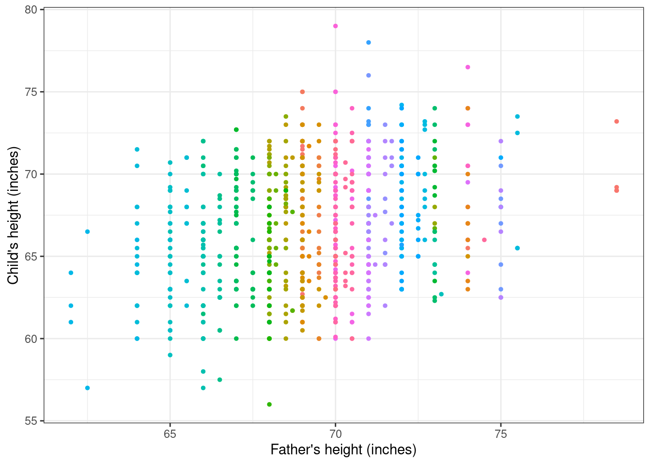
The data can be visualised by drawing a scatterplot, where the predictor (father’s height) is along the \(x-\)axis and the outcome (child’s age) is along the \(y-\)axis. This is presented in Figure 5.1, where each family is labelled by a different colour.
Galton’s objective was to find out whether there was some consistent relationship between the outcome and the predictor and, if so, to quantify the strength of this relationship. In developing his original work, he used a technique that was common at the time, called “least squares fitting”. The main idea underlying least squares fitting is that we would like to summarise a set of numbers \(y_1,\ldots,y_n\), by using a single value \(a\) and we would like to choose such a value \(a\) so that it is as close as possible to all the observed data points. One way to ensure this is to determine \(a\) as the solution of the equation \[ \min_{a} \left(\sum_{i=1}^n (y_i -a)^2\right) = \min_{a} \left((y_1-a)^2 + (y_2-a)^2 +\ldots + (y_n-a)^2\right). \tag{5.2}\]
The intuition behind the least squares ideas is that by minimising the sum of the square distances between each data point and the value \(a\), we ensure that the “prediction error” (i.e. the error we make in using the summary \(a\) instead of each true value \(y_i\)) is as small as possible, overall. If we consider the linear model in Equation 5.1, Equation 5.2 becomes \[\begin{eqnarray*} \min_{\boldsymbol\beta} \sum_{i=1}^n \left[y_i - \left(\beta_0 + \beta_1 X_{1i}\right) \right]^2 \end{eqnarray*}\] and, as it happens, we can prove that the optimal values for \(\boldsymbol\beta=(\beta_0,\beta_1)\) are \[\begin{eqnarray*} \hat\beta_1 = \frac{\mbox{Cov}(y,X_1)}{\mbox{Var}[X_1]} \qquad \mbox{ and } \qquad \hat\beta_0 = \bar{y}-\hat\beta_1 \bar{X}_1, \end{eqnarray*}\] where \[ \mbox{Cov}(y,X_1) = \frac{1}{n}\sum_{i=1}^n \left(X_{1i}-\bar{X}_1\right) \left(y_i - \bar{y} \right) \tag{5.3}\] is the covariance between the outcome \(y\) and the covariate \(X_1\), indicating a measure of joint spread around the means for the pair \((y,X_1)\).
If we use the observed data (which we assumed stored in a data.frame, named galton), we can compute the relevant quantites, e.g. in R using the following commands
y.bar=mean(galton$Height)
X1.bar=mean(galton$Father)
Cxy=cov(galton$Height,galton$Father)
Vx=var(galton$Father)
beta1.hat=Cxy/Vx
beta0.hat=y.bar-beta1.hat*X1.bar
which return the least square estimates for \(\hat\beta_0\) and \(\hat\beta_1\) as \[ \hat\beta_1=\frac{2.44}{6.10}=0.399 \qquad \mbox{ and } \qquad \hat\beta_0 = 66.76 - 0.399\times 69.23=39.11.\]
We can use these estimates to superimpose the regression line over the observed data, as shown in Figure 5.2.
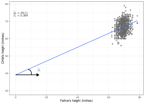
We have purposedly chosen to show the \(x-\) axis going all the way to the origin (\(x=0\)), even though the mass of points is actually very far from this point. This is not surprising — it is not very meaningful to imagine that we may have observed fathers whose height is equal to 0 inches! This highlights two important features when presenting data and, specifically, regression analyses:
- Plot the underlying data and/or the resulting regression curve on a suitable range. This should be dictated mostly by the scale or range of the observed data;
- It is often a good idea to re-scale the covariates. A useful re-scaling is to “centre” the covariates, by considering \(X^*_i = (X_i-\bar{X})\).
This is also related to the interpretation of the regression coefficients (at least for a linear regression), which is why we have used this sub-optimal pictorial representation. Figure 5.2 shows that the coefficient \(\hat\beta_0\) identifies the value of the line in correspondence with a covariate set to the value of 0. In other words, if we considered a father whose height is 0 inches, we would be predicting that his child’s height would be, on average, \(\hat\beta_0=39.11\) inches — i.e. the point along the \(y-\)axis in which the regression line crosses it. This is referred to as the intercept.
As for the second regression coefficient \(\hat\beta_1\), the graph in Figure 5.2 shows that this can be interpreted as the slope of the regression curve. That is the inclination of the line, as described by the angle shown in the left-hand side of the graph (the arc below the line). The interpretation of this feature is that \(\hat\beta_1\) is responsible for how much the line “tiltes” — if the estimated value is high, then the line becomes steeper, while if it is low, it becomes more shallow. When \(\hat\beta_1=0\), then the regression line is parallel to the \(x-\)axis, indicating the, irrespective of the value of the covariate \(X\), the expected value for the outcome \(y\) remains unchanged. This essentially indicates that if \(\hat\beta_1=0\) then \(X\) has no effect on \(y\).
If we compare two individuals whose \(X\) value differs by 1 unit (e.g. two fathers whose heights differ by 1 inch), the slope indicates the increase in the expected outcome (e.g. the expected height of their respective child). This can be easily seen by considering the linear predictor for two different fathers, say \(F_1\) and \(F_2\), for whom the recorded heights are, say, 70 and 71 inches, respectively. The expected heights for the childred of \(F_1\) and \(F_2\) are then \[\begin{eqnarray*} \mbox{E}[Y\mid X=71] = \beta_0 + \beta_1\times 71 \qquad \mbox{ and } \qquad \mbox{E}[Y\mid X=72] = \beta_0 + \beta_1\times 72. \end{eqnarray*}\] Thus, the difference between these two expected outcomes (i.e. the effect of a unit change in the father’s height) is \[\begin{eqnarray*} \Delta_X & = & \mbox{E}[Y\mid X=72] - \mbox{E}[Y\mid X=71] \\ & = & \left(\hat\beta_0 + \hat\beta_1\times 72\right) - \left(\hat\beta_0 + \hat\beta_1\times 71\right) \\ & = & \hat\beta_0 + \hat\beta_1\times 72 - \hat\beta_0 -\hat\beta_1\times 71 \\ & = & \hat\beta_1 (72-71) \\ & = & \hat\beta_1 = 0.399. \end{eqnarray*}\]
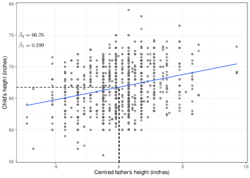
Figure 5.3 shows the original data on children’s height on the \(y-\)axis, along the centred version of their father’s data on the \(x-\)axis and with the new regression line superimposed. As is indicated in the graph, the slope \(\hat\beta_1\) is unchanged, while the intercept is indeed changed. That is because the change in the scale of the \(X\) covariate (which as is possible to see now goes from -7.23 to 9.27) is modified. The “effect” of the covariate on the outcome is not affected by this change of scale; however, we are now in a position of providing a better interpretation of the intercept: this is the value of the expected outcome in correspondence of a centred value for the covariate equal to 0. It is easy to see that if \(X^*_i=(X_i-\bar{X})=0\), then the original value \(X_i=\bar{X}\). So the intercept is the expected outcome for a father with the average height in the observed population — and this is something that may exist and certainly makes sense!
As you will see in more details if you take STAT0019, centring covariates is particularly important within a Bayesian setting, because this has the added benefit of improving convergence of simulation algorithms (e.g. Markov Chain Monte Carlo), which underpin the actual performance of Bayesian modelling.
The terminology “regression” comes from Galton’s original conclusion from his analysis — when plotting the original data with superimposed both the least square regression line (in blue in Figure 5.4) and the line of “equality” (the black line). This is constructed by using a slope equal to 0 and an intercept equal to 1, essentially implying that on average we expect children and their father to have the same height.
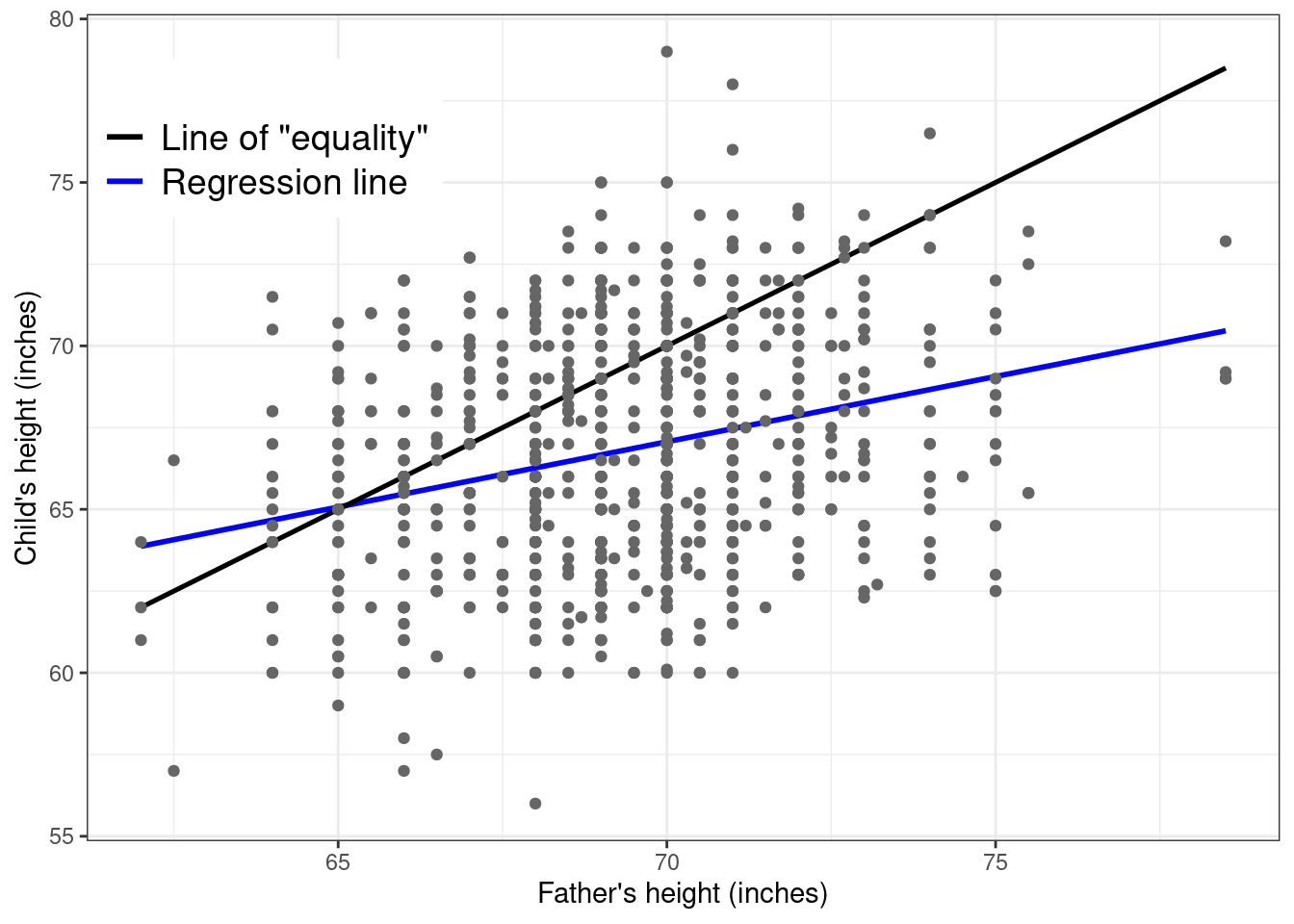
What Galton noted is that shorter fathers tended to be associated with slightly taller children. This is noticeable because at the left-hand of the \(x-\)axis, the blue curve (the estimated least squares regression) is higher than the line of equality. Conversely, if a father was taller, then on average his child(ren) tended to be shorter than him (because at the other extreme the black line is increasingly higher than the blue line). With his eugenist hat on, he found this rather disappointing, because it meant that the species could not be improved (e.g. by selecting only taller parents to breed). For this reason, he gave this phenomenon the rather demeaning name “regression to mediocrity” or “to the mean”.
5.2 Regression as a statistical model
Galton’s original analysis is not really framed as a full statistical model, because it is rather based on the idea of mathematical optimisation provided by the least squares. In fact, he did not specify explicitly any distributional assumption behind the data observed. From the statistical perspective, this is a limiting factor, because, for example, it is impossible to go beyond the point estimate of the regression coefficients, unless we are willing to provide some more expanded model, based on probability distributions.
In practice, this extension is fairly easy, as we will show in the following. In its simplest form, we can assume that the sampling variability underlying the observed data can be described by a Normal distribution. This amounts to assuming that \[ y_i \sim \mbox{Normal}(\mu_i,\sigma^2) \tag{5.4}\] \[ \mu_i = \beta_0 + \beta_1 X_{1i} + \ldots + \beta_K X_{Ki}. \tag{5.5}\] for \(i=1,\ldots,n\). This notation highlights the probabilistic nature of the assumed regression relationship between \(y\) and \(\boldsymbol{X}\): we are assuming that the linear predictor of Equation 5.1 is on average the best estimate of the outcome, given a specific “profile”, i.e. a set of values for the observed covariates. But we do not impose determinism on this relationship: there is a variance, which is determined by the sampling variability in the observed data and expressed by the population parameter \(\sigma^2\).
An alternative way of writing the regression model (which is perhaps more common in Econometrics than it is in Statistics) is to consider \[ y_i = \beta_0 + \beta_1 X_{1i} + \ldots + \beta_K X_{Ki} + \varepsilon_i, \quad \mbox{with} \quad \varepsilon_i \sim \mbox{Normal}(0,\sigma^2). \tag{5.6}\] Equation 5.6 explicitly describes the assumption mentioned above. The quantity \(\varepsilon_i\) represents some kind of “white noise”, or, in other words, a random error, that is centered on 0 and whose variance basically depends on the population variability.
5.2.1 Bayesian approach
The model parameters for the specification in Equation 5.4 and Equation 5.5 are the coefficients \(\boldsymbol\beta\) and the variance \(\sigma^2\). Thus, in order to perform the Bayesian analysis, we need to specify a suitable prior distribution for \(\boldsymbol\theta=(\boldsymbol\beta,\sigma^2)\). Ideally, we would specify a joint, multivariate prior \(p(\boldsymbol\theta)\), which would be used to encode any knowledge on the uncertainty about each parameter, as well as the correlation among them.
In practice, we often assume some form of (conditional) independence, where the \((K+2)\) dimensional distribution \(p(\boldsymbol\theta)\) is factorised into a product of simpler (lower-dimensional) distributions, exploiting some (alleged!) independence conditions among the parameters. For instance, we may model the regression coefficients independently on one another and on the population variance \[\begin{eqnarray*} p(\boldsymbol\theta)=p\left(\boldsymbol{\beta},{\sigma}^2\right) = p\left({\sigma}^2\right) \prod_{k=0}^K p(\beta_k). \end{eqnarray*}\]
This is of course just a convenient specification and care should be taken in encoding the actual prior knowledge into the definition of the prior distribution. Notice however that even if we are assuming some form of independence in the prior distribution, it is possible that in the posterior (i.e. after observing the evidence provided by the data), we have some level of correlation among (some of) the parameters.
There are of course many possible models we can define for the prior, but a convenient (if often relatively unrealistic) choice is to assume vague Normal priors on the coefficients: \((\beta_0,\beta_1,\ldots,\beta_K)\stackrel{iid}{\sim}\mbox{Normal}(0,v)\) with a fixed and large variance \(v\); and a Gamma distribution for the precision \(\tau=1/\sigma^2 \sim \mbox{Gamma}(a,b)\), for some fixed, small values \((a,b)\) — see for example Gelman et al. (2013).
As mentioned above, it is convenient, particularly within the Bayesian framework to consider a centred version of the covariates, where \(X^*_{0i}=X_{0i}\) and \(X^*_{ki}=(X_{ki}-\bar{X}_k)\), for \(k=1,\ldots,K\) (notice that we should not rescale the column of the predictors matrix corresponding to the intercept — in fact we want to keep it as a vector of ones, to ensure that the matrix multiplication returns the correct values). For example, using again Galton’s data, if we wanted to include in the model also the mothers’ heights (indicated as \(X_{2i}\)) and use a centred version of the covariates, then the linear predictor would be \[\begin{eqnarray*} \mu_i & = & \beta_0 X^*_{0i} + \beta_1 X^*_{1i} + \beta_K X^*_{2i}\\ & = & \boldsymbol{X}_i^* \boldsymbol\beta \end{eqnarray*}\] where \(\boldsymbol\beta=(\beta_0,\beta_1,\beta_2)\) and the predictors matrix \(\boldsymbol{X}^*\) is
\[\begin{equation*} \boldsymbol{X}^* = \left(\begin{array}{ccc} X_{01}^* & X_{11}^* & X_{21}^* \\ X_{02}^* & X_{12}^* & X_{22}^* \\ X_{03}^* & X_{13}^* & X_{23}^* \\ X_{04}^* & X_{14}^* & X_{24}^* \\ \vdots & \vdots & \vdots \\ X_{0n}^* & X_{1n}^* & X_{2n}^* \end{array}\right) = \left(\begin{array}{ccc} 1 & 9.27 & 2.92 \\ 1 & 9.27 & 2.92 \\ 1 & 9.27 & 2.92 \\ 1 & 9.27 & 2.92 \\ \vdots & \vdots & \vdots \\ 1 & -0.733 & 0.92 \end{array}\right). \end{equation*}\]
We may specify a prior for the father’s and mother’s effect that is fairly skeptical, by setting a Normal distribution, centred around 0 (indicating that on average we are not expecting an impact of these covariates on the predicted value of their child’s height), with a relatively large variance. For instance we could set \(\beta_1,\beta_2\stackrel{iid}{\sim}\mbox{Normal}(0,\mbox{sd}=10)\). Note that in this case, looking at the context, we may argue that a standard deviation of 10 is already “large enough” to avoid including too much information in the prior. The blue curve in Figure 5.5 shows a graphical representation of this prior.
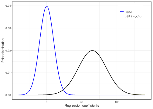
As for the intercept \(\beta_0\), given the centring in our model, this represents the expected height of a child whose mother and father’s heights are at the average in the population. We can use some general knowledge about people’s heights in Victorian times and, assuming no particular association between the outcome and the covariate, we may set a Normal prior with mean equal to 65 inches (approximately 165 cm) and standard deviation equal to 20. Again, we are not imposing a particular value for the intercept, in the prior, but while using a reasonable choice, we still maintain some substantial uncertainty before seeing the data. Notice that essentially this prior (correctly!) assigns 0 probability of negative heights — in fact heights below 20 inches are very unlikely under the model assumed.
Unfortunately, this model is not possible to compute in closed form and so in order to estimate the posterior distributions for the parameters, we need to resort to a simulation approach (e.g. Markov Chain Monte Carlo, MCMC — the details are not important here and you will see much more on this if you take STAT0019). The output of the model is presented in Table 5.2.
| mean | sd | 2.5% | 97.5% | |
|---|---|---|---|---|
| \(\beta_0\) (intercept) | 66.7545 | 0.1129 | 66.5296 | 66.9671 |
| \(\beta_1\) (slope for father’s height) | 0.3783 | 0.0458 | 0.2862 | 0.4690 |
| \(\beta_2\) (slope for mothers’s height) | 0.2832 | 0.0489 | 0.1888 | 0.3818 |
| \(\sigma\) (population variance) | 3.3906 | 0.0829 | 3.2328 | 3.5506 |
The computer output shows some summary statistics for the estimated posterior distributions of the model parameters. The posterior mean for the intercept is very close to our prior guess, but the uncertainty in the overall distribution is massively reduced by the observed data — the 95% interval estimate is indeed very narrow, ranging from 66.53 to 66.97.
As for the slopes \(\beta_1\) and \(\beta_2\), both have a positive mean and the entire 95% interval estimate is also above 0. This indicates that there seems to be a truly positive relationship between the heights of the parents and those of their offspring. Nevertheless, the magnitude of the effect is not very large, which explains the phenomenon so disconcerting for Galton.
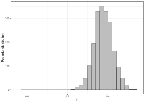
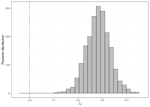
We can use a similar reasoning to that shown in Section 4.1 to determine, using the full posterior distributions, the probability that either \(\beta_1\) or \(\beta_2\) are negative (which would indicate the opposite relationship). These can be obtained numerically, using the output of the MCMC analysis. As is obvious from Figure 5.6, there is essentially no probability of either the two slopes being negative.
Finally, notice that the coefficients for the father’s height has now changed from the least square analysis given above. This is possibly due to the influence of the prior distribution, in the Bayesian analysis. Nevertheless, because we are now including an additional covariate, it is extremely likely that the effect of the father’s height be indeed modified in comparison to the simpler analysis, simply because of the joint variation brought about by the formal consideration of the mother’s height.
5.2.2 Likelihood approach
As shown in Section 3.1.2, the likelihood approach proceeds by computing the maximum likelihood estimator for the model parameters. In this case, using relatively simple algebra, we can prove that the MLE for the coefficients \(\boldsymbol\beta=(\beta_0,\beta_1,\ldots,\beta_K)\) are equivalent to the least square solutions (as seen in Section 3.1.3, the MLE has usually all the good frequentist properties and thus it is often selected as the best estimator in that framework too).
Expanding on the result shown above, in the most general case for a linear regression, where we consider \(K\) predictors, the MLEs are \[ \hat\beta_0 = \bar{y}-\left(\hat\beta_1\bar{X}_1 + \ldots + \hat\beta_K \bar{X}_K \right) = \bar{y}-\sum_{k=1}^K \beta_k \bar{X}_k \tag{5.7}\] \[ \hat\beta_1 = \frac{\mbox{Cov}(y,X_1)}{\mbox{Var}[X_1]} \tag{5.8}\] \[ \vdots \] \[ \hat\beta_K = \frac{\mbox{Cov}(y,X_K)}{\mbox{Var}[X_K]}. \tag{5.9}\]
In addition, the MLE for the population (sometimes referred to as “residual”) variance \(\sigma^2\) is given by \[ \hat\sigma^2 = \frac{\mbox{RSS}}{(n-K-1)}, \tag{5.10}\] where: \[\begin{eqnarray*} \mbox{RSS} & = &\sum_{i=1}^n \left(y_i - \hat{y}_i\right)^2 \\ & = & \sum_{i=1}^n \left(y_i - \left[\beta_0 + \beta_1 X_{1i} + \beta_2 X_{2i} + \ldots + \beta_K X_{Ki}\right]\right)^2 \end{eqnarray*}\] is the residual sum of squares, i.e. a measure of the “error” we make by estimating the outcome using the regression line (i.e. the residuals \(\hat{y}_i\)), instead of the actual observed points (\(y_i\)); and the denominator of Equation 5.10 is the degrees of freedom, which in the general case are equal to the number of data points (\(n\)) minus the number of regression coefficients \((K+1\), in this case).
In practical terms, matrix algebra can be used to programme these equations more efficiently and compactly. For example, including again in the model both the fathers’ and the mothers’ heights on the original scale (i.e. without centring the covariates), then the linear predictor would be \[\begin{eqnarray*} \mu_i & = & \beta_0 X_{0i} + \beta_1 X_{1i} + \beta_K X_{2i}\\ & = & \boldsymbol{X}_i \boldsymbol\beta \end{eqnarray*}\] where \(\boldsymbol\beta=(\beta_0,\beta_1,\beta_2)\) and the predictors matrix \(\boldsymbol{X}\) is
\[\begin{equation*} \boldsymbol{X} = \left(\begin{array}{ccc} X_{01} & X_{11} & X_{21} \\ X_{02} & X_{12} & X_{22} \\ X_{03} & X_{13} & X_{23} \\ X_{04} & X_{14} & X_{24} \\ \vdots & \vdots & \vdots \\ X_{0n} & X_{1n} & X_{2n} \end{array}\right) = \left(\begin{array}{ccc} 1 & 78.5 & 67.0 \\ 1 & 78.5 & 67.0 \\ 1 & 78.5 & 67.0 \\ 1 & 78.5 & 67.0 \\ \vdots & \vdots & \vdots \\ 1 & 68.5 & 65.0 \end{array}\right). \end{equation*}\]
Equations 5.7 — 5.9 can be written compactly in matrix algebra using the notation \[ \hat{\boldsymbol\beta} = (\boldsymbol{X}^\top \boldsymbol{X})^{-1} \boldsymbol{X}^\top \boldsymbol{y}. \tag{5.11}\]
The operator \(^\top\) indicates the transpose of a matrix. So if you have a matrix \[\begin{eqnarray*} \boldsymbol{X} = \left(\begin{array}{cc} a & b \\ c & d \end{array} \right), \end{eqnarray*}\] then \[\begin{eqnarray*} \boldsymbol{X}^\top = \left(\begin{array}{cc} a & c \\ b & d \end{array}\right), \end{eqnarray*}\] i.e. the transpose matrix is constructed by flipping around the rows and the columns (the first column becomes the first row, the second column becomes the second row, etc.).
Multiplying the transpose of a matrix by the original matrix is equivalent to summing the cross-products of the values in the matrix \[\begin{eqnarray*} \boldsymbol{X}^\top \boldsymbol{X} & = & \left(\begin{array}{cc} a & c \\ b & d \end{array}\right) \times \left(\begin{array}{cc} a & b\\ c & d \end{array}\right) \\ & = & \left(\begin{array}{cc} \left(a\times a + c\times c\right) &\hspace{5pt} \left(a\times b + c \times d\right) \\ \left(b \times a + d \times c\right) & \hspace{5pt} \left(b \times b + d \times d\right) \end{array}\right) \\ & = & \left(\begin{array}{cc} a^2+c^2 & \hspace{5pt} ab+cd \\ ba+dc & \hspace{5pt} b^2+d^2 \end{array}\right) \end{eqnarray*}\] So, if \(\boldsymbol{X}\) is the matrix of predictors \[\begin{eqnarray*} \boldsymbol{X}^\top\boldsymbol{X} & = & \left(\begin{array}{cccc} X_{01} & X_{02} & \ldots & X_{0n} \\ X_{11} & X_{12} & \ldots & X_{1n} \\ \vdots & \vdots & \ddots & \vdots \\ X_{K1} & X_{K2} & \ldots & X_{Kn} \end{array}\right) \times \left(\begin{array}{cccc} X_{01} & X_{11} & \ldots & X_{K1} \\ X_{02} & X_{12} & \ldots & X_{K2} \\ \vdots & \vdots & \ddots & \vdots \\ X_{0n} & X_{1n} & \ldots & X_{Kn} \end{array}\right) \\ & = & \left(\begin{array}{cccc} \displaystyle\sum_{i=1}^n X_{0i}^2 & \displaystyle\sum_{i=1}^n X_{0i}X_{1i} & \ldots & \displaystyle\sum_{i=1}^n X_{0i}X_{Ki} \\ \displaystyle\sum_{i=1}^n X_{1i}X_{0i} & \displaystyle\sum_{i=1}^n X_{1i}^2 & \ldots & \displaystyle\sum_{i=1}^n X_{1i}X_{Ki} \\ \vdots & \vdots & \ddots & \vdots \\ \displaystyle\sum_{i=1}^n X_{Ki}X_{0i} & \displaystyle\sum_{i=1}^n X_{Ki}X_{1i} & \ldots & \displaystyle\sum_{i=1}^n X_{Ki}^2\end{array}\right), \end{eqnarray*}\] which is equivalent to the computation made for the covariance in Equation 5.3. Note that, irrespective of the original dimension of a matrix, multiplying a transpose by the original matrix always produces a square matrix (i.e. one with the same number of rows and columns).
The matrix operator \(^{-1}\) is the generalisation of the division operation for numbers. So, much like for a number \(x\) the product \(x x^{-1}=\frac{x}{x}=1\), for matrices the inverse is such that for a square matrix \(\boldsymbol{X}\), pre-multiplying by the inverse matrix produces the identity matrix (i.e. one with ones on the diagonal and zeros everywhere else). \[\begin{eqnarray*} \boldsymbol{X}^{-1} \boldsymbol{X} = \boldsymbol{1} = \left(\begin{array}{cccccccccc} 1 & & & 0 & & & \ldots & & & 0 \\ 0 & & & 1 & & & \ldots & & & 0 \\ \vdots & & & \vdots & & & \ddots & & & \vdots \\ 0 & & & 0 & & & \ldots & & & 1\end{array}\right). \end{eqnarray*}\]
Intuitively, Equation 5.11 is made by multiplying the inverse of the sum of squares for the matrix \(\boldsymbol{X}\) (which is proportional to the variance) by the sum of cross-squared between \(\boldsymbol{X}\) and \(\boldsymbol{y}\) (which is proportional to the covariance). This is basically the same as constructing the ratio between the covariance of \(\boldsymbol{X}\) and \(\boldsymbol{y}\) and the variance of \(\boldsymbol{X}\), exactly as in Equation 5.3.
This matrix algebra can be programmed in R using the commands
# Constructs the matrix of predictors, including the first column of ones
# the second column with the fathers' heights and the third column with
# the mothers' heights, from the original dataset
X=cbind(rep(1,nrow(galton)),galton$Father,galton$Mother)

# Assigns a label 1,2,...,n to each row of the matrix X
rownames(X)=1:nrow(X)
# And then visualises X as in the equation above, e.g. using
X[c(1:4,nrow(X)),]
[,1] [,2] [,3]
1 1 78.5 67
2 1 78.5 67
3 1 78.5 67
4 1 78.5 67
898 1 68.5 65# Constructs the vector of outcomes with the children's heights
y=galton$Height
# Now computes the MLE for all the regression coefficients
beta=solve(t(X)%*%X)%*%t(X)%*%y(in R the built-in command solve(X) is used to compute the inverse of a square matrix X, while the function t(X) is used to transpose its matrix argument).
The code above returns the following values for the coefficients.
      MLE estimate
beta0   22.3097055
beta1    0.3798970
beta2    0.2832145
We can also prove that these are unbiased for the underlying regression coefficients \(\beta_0,\ldots,\beta_K\), i.e. \[\begin{eqnarray*} \mbox{E}[\hat\beta_0] = \beta_0, \mbox{E}[\hat\beta_1] = \beta_1, \ldots, \mbox{E}[\hat\beta_K] = \beta_K \end{eqnarray*}\] and, using the theory shown in Chapter 3, that the sampling distribution for the estimators of each \(\hat\beta_k\) (for \(k=0,\ldots,K\)) is given by Normal distributions where the mean is of course the underlying “true” coefficient \(\beta_k\) and the variance is given by \[ \mbox{Var}[\beta_k] = \hat\sigma^2 \left(\boldsymbol{X}^\top \boldsymbol{X}\right)^{-1} \] — the intuition behind this formula is that we rescale the estimate of the variance of the error \(\varepsilon_i\) by the variance in the covariates to provide the variance of the estimate of the effects (coefficients).
Using matrix notation to compute \(\mbox{RSS} = (\boldsymbol{y}-\boldsymbol{X}\hat{\boldsymbol\beta})^\top (\boldsymbol{y}-\boldsymbol{X}\hat{\boldsymbol\beta})\), in R we can compute these variances using the following commands
# Computes the Residual Sums of Squares
RSS=t(y-X%*%beta)%*%(y-X%*%beta)
# Computes the estimate of the standard deviation sigma
# NB: "nrow(X)"=number of rows in the matrix X, while
#     "ncol(X)"=number of columns in the matrix X
sigma2.hat=as.numeric(RSS/(nrow(X)-ncol(X)))

# Now computes the variance of the coefficients using the formula above
sigma2.beta=sigma2.hat*solve(t(X)%*%X)
# Now squares the elements on the diagonal (i.e. the variances of the three
# coefficients), to obtain the standard deviations
sigma.beta=sqrt(diag(sigma2.beta))
to produce the estimates for the three coefficients in \(\boldsymbol\beta\) as below.
      MLE estimate         sd
beta0   22.3097055 4.30689678
beta1    0.3798970 0.04589120
beta2    0.2832145 0.04913817
At this point, using Equation 3.8, we can substitute the MLE \(\hat\beta_k\) for \(\hat\theta\) and the estimate of the standard deviation of \(\hat\beta_k\) for \(\sigma/\sqrt{n}\) and compute a 95% interval for \(\hat\beta_k\) as \[ \left[\hat\beta_k -1.96 \sqrt{\mbox{Var}[\hat\beta_k]}; \hat\beta_k + 1.96 \sqrt{\mbox{Var}[\hat\beta_k]}, \right] \] which in the current case gives \[\begin{eqnarray*} \mbox{95\% interval for } \beta_0 & = & \left[22.31 -1.96\times4.31; 22.31 + 1.96\times4.31 \right] = \left[13.87; 30.75 \right] \\ \mbox{95\% interval for } \beta_1 & = & \left[0.38 -1.96 0.04590.38 + 1.96\times0.0459 \right] = \left[0.29; 0.47 \right] \\ \mbox{95\% interval for } \beta_2 & = & \left[0.283 -1.96 0.0491 0.283 + 1.96\times0.0491 \right] = \left[0.187; 0.38 \right] . \end{eqnarray*}\]
Similarly, because we know what the sampling distribution for each of the three estimates is, we can compute \(p-\)values, for instance against the null hypothesis \(H_0: \hat\beta_k=0\). Notice that this is really relevant just for the slopes (i.e. the effects of the covariates), because if the resulting \(p-\)value is small, then we would have determined some evidence against the hypothesis of “no effect” (e.g. of the fathers’ heights on their children’s height).
Recalling Equation 4.2, we can prove that, under \(H_0\), \[
T=\frac{\hat\beta_k-0}{\mbox{Var}[\hat\beta_k]} \sim \mbox{t}(0,1,(n-K-1)).
\tag{5.12}\] Because all the \(\hat\beta_k>0\), then the relevant tail-area probability is the one to the right of the underlying t sampling distribution and so the \(p-\)values are computed in R as the following
                       p-value
beta0 0.0000001371088497591075
beta1 0.0000000000000002260111
beta2 0.0000000056616890636972
(recall that the option lower.tail=FALSE computes the area to the right of a given distribution).
Because the \(p-\)values are all very small (and certainly much lower than the common threshold of 0.05), we can claim very strong evidence against \(H_0\) and so, in a purely Fisherian interpretation, we would advocate the presence of some effect of both fathers’ and mothers’ heights on the children’s height. In common parlance, the three coefficients are deemed to be “highly significant” at the 0.05 level.
This results is also consistent with the analysis of the 95% confidence intervals (cfr. Section 4.4.3). The \(p-\)values are all very small — and at the same time, all the 95% confidence intervals exclude the value 0, indicating that the results are “significant” (and in this case, positive).
Of course, in practice, you will never need to make matrix calculations by hand — or even programme them directly. Most likely you will use routines and programmes available in statistical software to do the regression analysis. For example, in R we can compute the regression coefficients using the built-in function lm, as in the following code.
# Runs the function "lm" to run the model including "Height" as the reponse
# (that is the variable to the left of the twiddle symbol "~"), while "Father"
# and "Mother" (the variables to the right of the twiddle) are the covariates.
# These are recorded in the dataset called "galton"
m1=lm(formula=Height~Father+Mother,data=galton)
# Now displays the output
summary(m1)
Call:
lm(formula = Height ~ Father + Mother, data = galton)

Residuals:
   Min     1Q Median     3Q    Max
-9.136 -2.700 -0.181  2.768 11.689

Coefficients:
            Estimate Std. Error t value Pr(>|t|)
(Intercept) 22.30971    4.30690   5.180 2.74e-07 ***
Father       0.37990    0.04589   8.278 4.52e-16 ***
Mother       0.28321    0.04914   5.764 1.13e-08 ***
---
Signif. codes:  0 '***' 0.001 '**' 0.01 '*' 0.05 '.' 0.1 ' ' 1

Residual standard error: 3.386 on 895 degrees of freedom
Multiple R-squared:  0.1089,    Adjusted R-squared:  0.1069
F-statistic: 54.69 on 2 and 895 DF,  p-value: < 2.2e-16
The standard output reported by R includes the estimates for the coefficients (the column labelled as Estimate), their standard error based on the suitable sampling distributions (the column labelled Std. Error) and the value of the test statistic \(T\) of Equation 5.12 in the column labelled as t value.
Notice that by default, lm reports the \(p-\)value computed for an implicit alternative hypothesis \(H_1: \beta_k \neq 0\) (see the discussion in Section 4.4.1). For this reason, the \(p-\)values reported by lm in the column labelled as Pr(>|t|) are different than the one we have computed above. If we multiply by 2 the \(p-\)values above (to account for the difference than implicit in the alternative hypothesis, as opposed to simply the tail-area probability under the sampling distribution in correspondence with \(H_0\)), we obtain
           p-value
beta0 2.742177e-07
beta1 4.520223e-16
beta2 1.132338e-08
which are in fact consistent with the table reported by lm. To highlight the fact that these \(p-\)value are highly significant, lm uses a “star-based” rating system — where *** indicates that a \(p-\)value is between 0 and 0.001, ** that it is between 0.001 and 0.01, * that it is between 0.01 and 0.05 and . that it is between 0.05 and 0.1.
The analysis based on the MLE and \(p-\)values shows some slight discrepancies with the Bayesian analysis shown above. By and large the results are extremely consistent — notice that because of the different scaling of the covariate, the intercepts \(\beta_0\) are not directly comparable. As for the slopes (which, on the contrary are directly comparable), the Bayesian analysis estimates the effect of fathers’ height to be 0.3783, while the frequentist model indicates a value of 0.3799. For the mothers’ height effect, the Bayesian model estimates 0.2832, while the MLE-based analysis indicates that it is 0.2832. More importantly, all the coefficients are estimated with large precision, so that the entire intervals are above 0, in both approaches.
In this case, because we have a relatively large dataset, with evidence that consistently points towards the same direction; and we have used relatively vague priors, the numerical outputs of the two approaches are highly comparable. But this need not be the case in general, particularly when the data size is small and they provide only limited evidence. From the Bayesian point of view, this is perfectly reasonable: if we do not have overwhelming evidence, it is sensible that including prior knowledge does exert some influence on the final decisions.
This feature is also particular important when we need to complement limited evidence from observed data (e.g. in terms of short follow up, or large non-compliance).
5.3 Generalised linear regression
One of the main assumptions underlying the linear regression analysis seen above when viewed as a statistical model is that the underlying outcome is suitably modelled using a Normal distribution — this implies that we can assume that \(Y\) is reasonably symmetric, continuous and unbounded, i.e. it can, at least theoretically, take on values in the range \((-\infty; \infty)\).
However, as we have seen in Chapter 2, there are many cases in which variables are not suitably described by a Normal distribution — notably Bernoulli/Binomial or Poisson counts, but (as you will see if you take STAT0019) also other variables describing skewed phenomena (e.g. costs or times to event). In these instances, we can slightly extend the set up of Equation 5.4 and Equation 5.5 to account for this extra complexity. This can be accomplished using the following structure. \[ \left\{ \begin{array}{ll} y_i \stackrel{iid}{\sim} p(y_i \mid \boldsymbol\theta_i, \boldsymbol{X}_i) & \mbox{is the model to describe sampling variability for the outcome} \\ \boldsymbol\theta_i = (\mu_i,\boldsymbol\alpha) & \mbox{is the vector of model parameters} \\ \mu_i = \mbox{E}[Y_i \mid \boldsymbol{X}_i] & \mbox{is the mean of the outcome given the covariates $\boldsymbol{X}_i$} \\ \boldsymbol\alpha & \mbox{is a vector of other potential model parameters, e.g. variances, etc.} \\ & \mbox{(NB this may or may not exist for a specific model)} \\ g(\mu_i) = \boldsymbol{X}_i \boldsymbol\beta & \mbox{is the linear predictor on the scale defined by $g(\cdot)$}. \end{array} \right. \tag{5.13}\]
A function such that \(g(x)=x\) is referred to as the identity function. We can see that linear regression, presented in Section 5.2, is in fact a special case of the wider class of structures described in Equation 5.13, which is often referred to as Generalised Linear Models (GLMs). A GLM in which \(p(y_i\mid \boldsymbol\theta,\boldsymbol{X})=\mbox{Normal}(\mu_i,\sigma^2)\) and \(g(\mu_i)=\mu_i=\mbox{E}[Y\mid \boldsymbol{X}_i]=\boldsymbol{X}_i\boldsymbol\beta\) is the linear regression model of Equation 5.4 and Equation 5.5.
Upon varying the choice of the distribution \(p(\cdot)\) and the transformation function \(g(\cdot)\), we can model several outcomes.
5.3.1 Logistic regression
When the outcome is a binary or Binomial variable, we know that the mean \(\theta\) is the probability that a random individual in the relevant population experiences the event of interest. Thus, by necessity, \(\theta_i=\mbox{E}[Y_i\mid\boldsymbol{X}_i]\) is bounded by 0 from below and 1 from above (i.e. it cannot be below 0 or above 1). For this reason, we should not use a linear regression to model this type of outcome (although sometimes this is done, particularly in Econometrics, in the context of “two-stage least square analysis”, which you may encounter during your studies).
One convenient way to model binary outcomes in a regression context is to use the general structure of Equation 5.13, where the outcome is modelled using \(y_i \stackrel{iid}{\sim} \mbox{Bernoulli}(\theta_i)\) and \[ g(\theta_i) = g\left(\mbox{E}[Y_i\mid\boldsymbol{X}_i]\right) = \mbox{logit}(\theta_i)=\log\left(\frac{\theta_i}{1-\theta_i}\right) = \boldsymbol{X}_i \boldsymbol\beta \tag{5.14}\] (notice that in the Bernoulli model there is only one parameter and so we indicate here \(\boldsymbol\theta=\theta\)).
Equation 5.14 is referred to as logistic regression. Figure 5.7 shows graphically the mapping from the original range of the parameter \(\theta\), on the \(x-\)axis, to the rescaled parameter \(g(\theta)=\mbox{logit}(\theta)\), on the \(y-\)axis. As is possible to see, the original range is mapped onto the whole set of numbers from \(-\infty\) (in correspondence of the value \(\theta=0\)) to \(\infty\) (for \(\theta=1\)).
Registered S3 methods overwritten by 'bmhe':
  method      from
  print.bugs  R2WinBUGS
print.rjags R2jags 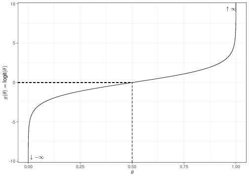
This is obvious by noting that \[\begin{eqnarray*} \theta=0 & \Rightarrow & \log\left(\frac{\theta}{1-\theta}\right) = \log\left(\frac{0}{1}\right) = \log(0) \rightarrow -\infty \end{eqnarray*}\] and \[\begin{eqnarray*} \theta=1 & \Rightarrow & \log\left(\frac{\theta}{1-\theta}\right) = \log\left(\frac{1}{0}\right) = \log(\infty) \rightarrow \infty. \\ \end{eqnarray*}\]
In addition, the graph in Figure 5.7 shows that the resulting function of \(\theta\) is reasonably symmetric around the central point (\(\theta=0.5\)).
If \(\theta\) represents a probability (e.g. that a given event \(E\) happens), the quantity \[\mbox{O}= \left(\frac{\theta}{1-\theta}\right) = \frac{\Pr(E)}{1-\Pr(E)}\] is called the odds for the event \(E\) and it represents a measure of how more likely \(E\) is to happen than not. If \(\Pr(E)=\theta=0.5\), then \(\displaystyle\mbox{O}=0.5/0.5=1\). If \(\Pr(E)\) is small, then O is also very small, while if \(E\) is very likely, then O is increasingly bigger. The range in which O is defined is characterised by the extreme values 0 (in correspondence of which \(E\) is impossible, i.e. \(\Pr(E)=0\) and thus \(\displaystyle \mbox{O}=0/1=0\)) and \(\infty\), when \(E\) is certain, i.e. \(\Pr(E)=1\) and thus \(\displaystyle \mbox{O}=1/0=\infty\).
The quantity \(\displaystyle \log\left(\frac{\theta}{1-\theta}\right) = \log\mbox{O}\) is the log-odds for the event \(E\). By applying the log transformation to O, we map its range in the interval \([\log(0)=-\infty; \log(\infty)=\infty]\).
Equation 5.14 clarifies that logistic regression implies that we are modelling the log-odds using a linear predictor or, in other words, that we are assuming a linear relationship between the mean outcome and the covariates, on the log odds scale.
For example, consider again Galton’s data, but this time, our outcome is given by a new variable, which takes value 1 if the original child’s height is above a threshold of 71 inches (180 cm) and 0 otherwise. We can create the suitable data in R using the following command.
# Creates a variable "y2" taking value 1 if the original child's height > median
y2=ifelse(galton$Height>71,1,0)
# Summarises the new variable
table(y2)
y2
0 1
801 97 As is possible to see, nearly 10.80% (i.e. 97/898) of the sample “experiences the event”, i.e. is taller than the set threshold.
The interpretation of the regression coefficients in a logistic regression needs a bit of care, given the change in the scale we define for the linear predictor.
The intercept is still related to the expected mean of the outcome for the profile of covariates all set to 0. So, in Galton’s example, centering the covariates for simplicity of interpretation, this would be the expected value for the height of a child of “average” father and mother (in terms of height). However, this time the expected mean of the outcome is the probability of the underlying event of interest, e.g. that a child is taller than the threshold of 71 inches. So, for an individual with centred covariates set to 0 (e.g. for a child whose parents’ centred height is 0), then the regression line (on the log-odds scale) is simply \[\begin{eqnarray*} \mbox{logit}(\theta_i) = \log\left(\frac{\theta_i}{1-\theta_i}\right) = \beta_0 \end{eqnarray*}\] and thus, recalling that \(\exp\left(\log\left(x\right)\right)=x\), we can invert the logit function to give \[ \begin{array}{ll} & \exp\left[\log\left(\frac{\theta_i}{1-\theta_i}\right)\right] = \exp\left(\beta_0\right) \Rightarrow \\ & \theta_i = \exp\left(\beta_0\right) (1-\theta_i) \Rightarrow \\ & \theta_i\left[1+\exp\left(\beta_0\right)\right] = \exp\left(\beta_0\right) \Rightarrow \end{array} \] \[ \theta_i = \frac{\exp\left(\beta_0\right)}{1+\exp\left(\beta_0\right)} \tag{5.15}\] (the right hand side of Equation 5.15 is often referred to as the expit or inverse logit transformation). This particular rescaling of intercept represents the expected mean outcome (= the probability that the event under study occurs, for an individual with covariates set to 0 — or to the overall average, if we are centring them).
The “slope” has also a slightly different interpretation in a logistic regression. We have seen before that a generic slope \(\beta_k\) represents the difference in the expected outcome for two individuals whose \(k-\)th covariate varies by one unit, “all else being equal”, i.e. where all the other covariates are set to the same value.
For instance, if in the current example we compared two fathers, one for whom the centred height was 0 (= 69.23 inches) and one for whom the centred height was 1 (= 70.23 inches), then we would have \[ \mbox{logit}(\theta \mid X^*_1=0) = \beta_0 + \beta_1 \times 0 = \beta_0, \] for the first one; and \[ \mbox{logit}(\theta \mid X^*_1=1) = \beta_0 + \beta_1 \times 1, \] for the second one. The difference between the expected outcomes would then be \[\begin{eqnarray*} \Delta_X & = &\mbox{logit}(\theta\mid X^*_1=1) - \mbox{logit}(\theta\mid X^*_1=0) \\ & = & \log\left(\frac{\theta}{1-\theta}\mid X^*_1=1 \right) - \log\left(\frac{\theta}{1-\theta}\mid X^*_1=0 \right) \\ & = & \log\left(\frac{\theta_1}{1-\theta_1}\right) - \log\left(\frac{\theta_0}{1-\theta_0}\right) \\ & = & (\beta_0 + \beta_1) - (\beta_0) \\ & = & \beta_1, \end{eqnarray*}\] indicating the probability of the event in correspondence of the covariate profile \(X_1^*=j\) (for \(j=0,1\)) with the notation \(\theta_j\), for simplicity.
Recalling that for any two positive numbers \((a,b)\) we can show that \(\log(a)-\log(b)=\log\left(a/b\right)\), we can then write \[\begin{eqnarray*} \log\left(\frac{\theta_1}{1-\theta_1} \middle/ \frac{\theta_0}{1-\theta_0}\right) = \beta_1 \end{eqnarray*}\] The quantity \(\displaystyle \left(\frac{\theta_1}{1-\theta_1} \middle/ \frac{\theta_0}{1-\theta_0}\right)\) is the ratio of two odds — this is called the odds ratio (OR) and describes how much more likely an event \(E\) is to happen among those individuals who present the characteristic associated with \(X^*_1=1\) (which happens with probability \(\theta_1\)) than among those who have \(X^*_1=0\) (which is associated with probability \(\theta_0\)). Taking the log of this quantity gives the log-OR, which we can now see is the same as the value of the slope \(\beta_1\).
Theoretically, the log-OR ranges between \(-\infty\) and \(+\infty\), with larger values indicating that the event is more likely to happen when individuals are associated with larger values of the covariate. In this case, the taller the father, the more likely their child to be taller than 71 inches, by an amount \(\exp(\beta_1)\).
In general, negative values for a log-OR indicate that the covariate is negatively associated with the outcome, while positive log-OR suggest that the covariate is positively associated with the outcome. If we transform this on to the natural scale by exponentiating the log-OR, which means that OR\(\in [0,\infty)\), we can interpret an OR \(>1\) to indicate that the covariate has a positive effect on the (probability of the) outcome, while if OR \(<1\) then the opposite is true. When log-OR \(=0\) (or, equivalently OR \(=1\)), then there is no association between the covariate and the outcome.
5.3.1.1 Bayesian approach
In a Bayesian context, theoretically the model of Equation 5.14 does not pose particular problems: we need to specify prior distributions on the coefficients \(\boldsymbol\beta\) and, much as in the case of linear regression, we can use Normal distributions — note that Equation 5.14 is defined on the log-odds scale, which as suggested above, does have an unbounded range, which makes it reasonable to assume a Normal distribution for the coefficients.
Equation 5.15 is helpful when we want to set up a prior distribution for \(\beta_0\) in a meaningful way for the main parameter \(\theta\). For example, imagine we wanted to encode the assumption that, before getting to see any data, we expected only a 5 to 20% chance for a random person in the population to be taller than 71 inches. If we set a Normal(logit(0.105),sd=0.4) for \(\beta_0\), then we can check that what we are actually implying is a prior for the underlying “baseline” probability (i.e. for the child of “average” parents) as the one represented in Figure 5.8.
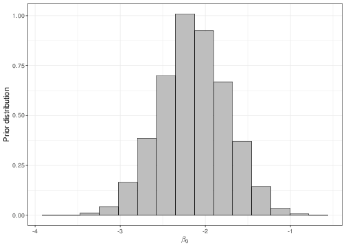
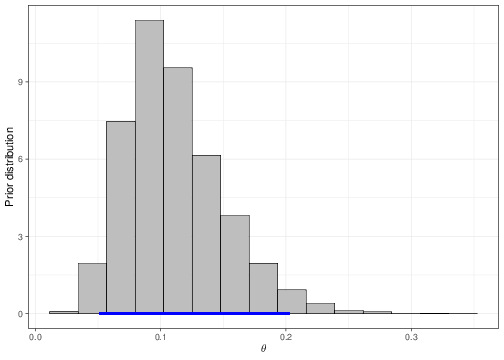
The dark blue horizontal line just above the \(x-\)axis in panel (b) indicates the 95% prior interval estimate for the parameter \(\theta\), which is derived by the prior depicted in panel (a). As is possible to see, the current choice for the mean and standard deviation of the Normal prior do induce a 95% interval covering approximately the required range. The values for the parameters of the Normal prior distribution for \(\beta_0\) can be found by trial-and-error, e.g. using the following R code:
# Defines the mean and sd of the prior
b0=log(0.105/(1-0.105))
s0=0.4
# Simulates 10000 values from the prior
beta0=rnorm(10000,b0,s0)
# Rescales the prior to the scale of the main parameter theta
theta=exp(beta0)/(1+exp(beta0))
# Checks the implied 95% interval estimate for theta
cbind(quantile(theta,.025),quantile(theta,.975))
[,1] [,2]
2.5% 0.05049197 0.2023662and changing the imposed value for b0 and s0 until the resulting approximate 95% interval returns values close enough to the required limits (5-20%). This procedure is often referred to as forward sampling. Note that setting some mildly “informative” prior for the intercept may be helpful in stabilising the inference, particularly when the data are made by only few records (i.e. small sample size), or, even more importantly, when the number of observed “successes” is small.
As for the slopes, we may elicit some informative prior and encode genuine prior knowledge in the model — for example, we may have some strong belief in a given treatment effect and thus we may set up a prior for the corresponding coefficient that is concentrated above 0. This would indicate a large prior probability that the resulting OR is greater than 1 and thus a positive association between the treatment and the outcome. However, in general terms, we may be unwilling to specifiy too strong a prior on a given treatment effect because we would like to be a bit more conservative and let the data drive the inference on this particular relationship.
For example we could set up \(\beta_1,\beta_2 \stackrel{iid}{\sim}\mbox{Normal}(0,sd=2)\). This assumes that, before seeing any data, we are not expecting a particular effect of either father’s or mother’s height on the probability of a child being taller than 71 inches (because these distributions are centred around 0 — recall that \(\beta_1\) and \(\beta_2\) represent the log-ORs!). However, we are implying some variance around it to guarantee the possibility that the effect is either positive or negative.
Notice that we are imposing a standard deviation of 2 — you may think that this is rather strict and we are in fact including some strong prior on these distributions. However, recall that the slopes are defined on the log-odds scale and so a value of 2 for a standard deviation is actually pretty large, when rescaled back to the original probability scale. Adapting Equation 3.8, we know that for a Normal distribution with mean 0 and standard deviation of 5, 95% of the probability is approximately included in the interval \([-1.96\times 2; 1.96\times 2] = [-3.92; 3.92]\), which when we map back on to the probability scale applying the inverse logit transformation implies a prior 95% interval for the OR of \([0.0198;50.40]\). That is extremely vague!
While we do not want to impose too strong priors on the “treatment effect”, there is much information that we can use to restrict the reasonable range of a log-OR.
For instance, consider an experiment in which you test the effectiveness of parachutes, when jumping off a flying plane. You define your outcome \(Y\) as 0 if the individual jumps off the plane and dies and 1 if they survive. You also have a covariate \(X_i\) taking value 1 if individual \(i\) is given a parachute and 0 otherwise.
In a situation such as this, you may expect the treatment to have a very large effect — almost everyone with a parachute can be reasonably expected to survive, while almost (or probably just!) everyone without one is most likely to die. So if you define \(\theta_1=\Pr(Y=1 \mid X=1)\) and \(\theta_0=\Pr(Y=1 \mid X=0)\), we could reasonably estimate something like \(\theta_1 =0.9\) and \(\theta_0=0.1\) (the actual numbers are irrelevant — but the magnitude is important and arguably realistic). Thus, in this case the OR would be \[\begin{eqnarray*} \mbox{OR} & = & \left. \frac{\theta_1}{1-\theta_1}\middle / \frac{\theta_0}{1-\theta_0} \right. \\ & = & \left. \frac{0.9}{1-0.9} \middle / \frac{0.1}{1-0.1} \right. \\ & = & \left. \frac{0.9}{0.1}\middle / \frac{0.1}{0.9} \right. = \left. 9 \middle / \frac{1}{9} \right. = 81. \end{eqnarray*}\] This means that people with a parachute are 81 times more likely to survive the jump off the plane than those without a parachute. This massive OR comes about, of course, because of the assumptions we are making about such a large treatment effect — almost everyone without the parachute dies, while almost everyone with survives. In a case such as this, we may be prepared to believe a very large OR. But in most cases, interventions do not have such dramatic effects. And thus, it is reasonable to imagine that ORs greater than 3 or perhaps 4 are already relatively unlikely to be observed in practice!
Interestingly, there is no closed form for the posterior distributions of the model parameters, in a logistic regression. Thus we need to resort to simulations, e.g. MCMC. The details of the MCMC model used to run the analysis are not important here, but the results are summarised in Table 5.3.
| mean | sd | 2.5% | 97.5% | |
|---|---|---|---|---|
| \(\beta_0\) (intercept) | -0.0719 | 0.0687 | -0.2010 | 0.0605 |
| \(\beta_1\) (logOR for father’s height) | 0.1676 | 0.0303 | 0.1087 | 0.2283 |
| \(\beta_2\) (logOR for mothers’s height) | 0.0987 | 0.0304 | 0.0376 | 0.1595 |
In a logistic regression, typically we do not worry too much about the intercept (given the caveat above and the rescaling necessary to make sense of its value in terms of the underlying probability of “success”). As for the log-ORs, we can see that both the covariates are associated with a positive point estimate and both the entire 95% interval estimates are also positive, thus indicating a probability \(\geq 0.95\) that the posterior distributions of \(\beta_1\) and \(\beta_2\) are positive.
Of course, once we have the simulations for the log-OR, we can simply exponentiate each simulated values to obtain a full posterior distribution for the ORs. So for example if we had stored the output of the MCMC model in two suitable objects called beta1 and beta2, then we could simply rescale them to compute numerically probabilities associated with them, for example as in the following R code.
# Constructs the ORs from the original simulations obtained by the model
OR1=exp(beta1)
OR2=exp(beta2)
# Tail-area probability to estimate Pr(OR1<1). This is the proportion of
# simulations for OR1 that are below 1
sum(OR1<1)/length(OR1)
[1] 0# Tail-area probability to estimate Pr(OR2<1). This is the proportion of
# simulations for OR2 that are below 1
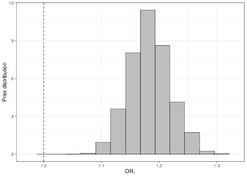
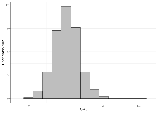
sum(OR2<1)/length(OR2)[1] 0.0005Once the objects OR1 and OR2 are available, we could plot histograms of the posterior distributions, as shown in Figure 5.9. As is possible to see, in both cases, none or very little of the posterior distribution is below 1, indicating a “highly significant” result in terms of the positive association between the covariates and the outcome.
5.3.1.2 Likelihood approach
If we consider a Likelihod approach, the idea is of course to maximise the likelihood function for the model parameters, to determine the MLE, which, again, would be considered a very good candidate for optimality even under a pure Frequentist approach. Unfortunately, for a logistic regression model, it is not possible to obtain maximum values analytically. Thus, we resort to numerical maximisation — usually based on a clever approximation method referred to as Newton-Rapson algorithm.
In practice, we do not need to programme this algorithm ourselves, but rather we rely on existing routines or programmes. For example R has a built-in command glm, that can be used to obtain the MLEs for GLMs.
The following code shows how to perform a GLM analysis for the model shown in Section 5.3.1.1 — all the assumptions are identical, except of course that we do not specify any prior distribution in this case.
Call:
glm(formula = formula, family = "binomial", data = data.frame(y2,
    X))

Deviance Residuals:
    Min       1Q   Median       3Q      Max
-1.7428  -1.1254  -0.7077   1.1306   1.6407

Coefficients:
            Estimate Std. Error z value     Pr(>|z|)
XIntercept -0.008175   0.068537  -0.119      0.90506
XFather     0.166414   0.029209   5.697 0.0000000122 ***
XMother     0.097989   0.030380   3.225      0.00126 **
---
Signif. codes:  0 '***' 0.001 '**' 0.01 '*' 0.05 '.' 0.1 ' ' 1

(Dispersion parameter for binomial family taken to be 1)

    Null deviance: 1244.9  on 898  degrees of freedom
Residual deviance: 1197.1  on 895  degrees of freedom
AIC: 1203.1

Number of Fisher Scoring iterations: 4
The computer output is fairly similar to that presented for the outcome of lm in the case of a linear regression. The main parameters are presented in the core of the table in terms of the point estimate (labelled as Estimate), the standard deviation (Std. Error), the value of the test statistic used to test the null hypothesis that each is equal to 0 (z value) and the “two-sided” \(p-\)value (indicated as Pr(>|z|) — see the discussion at the end of Section 5.2.2).
In this particular instance, the results are fairly similar to the numerical output of the Bayesian analysis. The intercept shows some slight differences — this is mainly due to the informative prior used above. However, for the two slopes, given that the prior was centred around 0 and in fact fairly vague, the effects of the covariates is estimated to very similar numerical values. Even the analysis of the \(p-\)values is consistent with the Bayesian analysis, in this case — the effect of the father’s height is more “significant”, much as the posterior distribution for \(\beta_1\) had shown a lower probability of being less than 0 in the Bayesian model.
Notice that unlike in the case of the linear regression, the \(p-\)values are computed this time based on a Wald test (see Section 4.4.4), computed as the ratio of the MLE minus the null value (0, in this case) to its standard deviation. So for example, in this case, the test statistic for \(X_2\) (the mother’s effect) can be computed as \[\begin{eqnarray*}
W & = & \frac{\hat\theta-0}{\sqrt{\mbox{Var}[\hat\theta]}} = \frac{0.098}{0.0304} = 3.225,
\end{eqnarray*}\] as shown in the computer output. We can compare this to the standard Normal to determine the \(p-\)value. In particular, as mentioned above, R constructs the two-sided version of the \(p-\)value, essentially using the following code.
# Stores the summary of the model output in the object "s"
s=summary(model)
# Constructs the W statistic using the elements of the object "s"
w=s$coefficients[3,1]/s$coefficients[3,2]
# Computes the two-sided p-value based on Normal(0,1) approximate distribution
P=2*(pnorm(q=w,mean=0,sd=1,lower.tail=FALSE))
# Prints the output (which is the same as in the computer output)
P
[1] 0.0012578775.3.2 Poisson and other GLMs
Logistic regression is only one of the models embedded in the wider family of GLMs. The general principles are essentially the same in all circumstances — specify a distribution \(p(y_i\mid\boldsymbol{\theta}_i, \boldsymbol{X}_i)\) and a suitable map from the natural scale of the mean to an unbounded range, where we can claim at least approximately linearity in the covariates.
Another common example is Poisson regression, where we have observed data on the outcome \(y_1,\ldots,y_n\stackrel{iid}{\sim}\mbox{Poisson}(\theta_i)\). Here the parameter \(\theta_i\) represents at once the mean and the variance of the underlying Poisson distribution. Because \(\theta_i\geq 0\) (as it represents a rate, i.e. the intensity with which the counts are observed), a suitable transformation is simply to take the log and model \[\begin{eqnarray} g(\theta_i) = g\left(\mbox{E}[Y_i\mid\boldsymbol{X}_i]\right)=\log(\theta_i) = \boldsymbol{X}_i\boldsymbol\beta. \end{eqnarray}\] In comparison to logistic regression, the interpretation of the coefficients is slightly simpler: using a reasoning similar to that shown for the intercept and slope of a logistic regression, we can show that, in the case of a Poisson GLM:
- The intercept \(\beta_0\) is the log rate for an individual whose covariates are set to 0;
- The slope \(\beta_k\) is the log relative risk corresponding to increasing the covariate by one unit. So if you compare two individuals, the first of whom has the value of the covariate \(X_k=1\) and the other for whom \(X_k=0\), then \(\beta_k=\log\left(\frac{\theta_1}{\theta_0}\right)\), where \(\theta_j\) is the rate associated with a covariates profile of \(X_k=j\), for \(j=0,1\).
The log-linear model embedded in the Poisson structure can be applied to several other distributions to describe sampling variability in the observed outcome. Other relevant examples include the case of time-to-event outcomes, for which suitable models are Weibull or Gamma, among others. Because all of these are defined as positive, continous variables, their mean is also positive and so it is useful to rescale the linear predictor on the log scale.
Galton was another very controversial character. He was a polyscientist, who made contributions to Statistics, Psychology, Sociology, Anthropology and many other sciences. He was the half-cousin of Charles Darwin and was inspired by his work on the origin of species to study hereditary traits in humans, including height, which he used to essentially invent regression. He also established and then financed the “Galton Laboratory” at UCL, which Karl Pearson went on to lead. Alas, Galton was also a major proponent of eugenics (in fact, he is credited with the invention of the term) and has thus left a troubling legacy behind him.↩︎