2 Statistical distributions: working with probability calculus

The objective of this chapter is to present a brief introduction to the use of some probability distributions to model sampling variability in observed data. For now, we consider a situation very simular to the one discussed in the context of Figure 1.1: we assume that there is a data generating process (DGP), i.e. a way in which data can arise and become available to us. This DGP determines the way in which some units are actually sampled from the theoretical target population.

As mentioned in Chapter 1, there are many different ways in which we can obtain a sample of \(n\) individuals out of the \(N>>n\) that make up the whole population. In a nutshell (and somewhat making a more trivial argument than it really is), the ideas we explore in this chapter assume that we can safely assume a DGP characterised by a probability distribution; often, we use the phrase “the variable \(y\) has a XXX distribution”. While this terminology is almost ubiquitous in Statistics and Probability Calculus, it is in fact slightly misleading. What we really mean is a rather handy shortcut for the much more verbose (and correct!) phrasing

“We can associate the observed data with a XXX distribution to describe our level of uncertainty, e.g. on the sampling process that has determined the actual observation we have made (or we will make in the future).”

Of course, it would be very impractical to always use this mouthful sentence — and practically nobody does. But: it is important to understand that probability distributions or DGPs are not physical properties of the data — that is why the data cannot have a probability distribution. Rather, they are mathematical idealised concepts that we use to represent complex phenomena in a convenient way.

In general, the DGP will depend on a set of parameters (which in general we indicate with Greek letters, e.g. \(\theta\), \(\mu\), \(\sigma\), \(\lambda\), etc). The distribution is characterised by a mathematical function, something like \[p(y\mid\theta_1,\theta_2,\theta_3)=\theta_1 \frac{\theta_2}{\sqrt{\theta_3}}\exp\left(\frac{(y-\theta_2)^2}{\log(\theta_3)}\right) \] (the actual form of this function is irrelevant here and this specific one is only chosen to make a point!). In this case, the parameters are \(\boldsymbol\theta=(\theta_1,\theta_2,\theta_3)\) and, given a specific value for them, we determine a certain value of the underlying probability distribution for the observable outcomes, \(y\). In other words, we can use a probability distribution to describe the chance that a specific outcome arises, given a set values of the parameters.

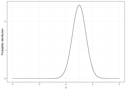
For example, for the fake distribution above, if \(\boldsymbol\theta=(2,1,0.6)\), then \(p(y)=2.582\exp\left( \frac{(y-1)^2}{-0.5108} \right)\). The graph in Figure 2.1 shows a graphical representation of the distribution \(p(y)\) for the set values of \(\boldsymbol\theta\). In this case, we are implying that the probability is distributed around a central part (more or less in correspondence of the value 1 along the \(x-\)axis) and that values increasingly further away are associated with very small probability weight (and thus are deemed unlikely by this model).

Figure 2.1: A graphical example of a probability distribution for a given set of value for the parameters \(\boldsymbol\theta\)

Of course, the assumption that we know the value of the parameters is certainly a big one and, in general, we are not in a position of having such certainty. And that is the point made in Figure 1.2 — instead of going from left to right, in reality we will try and go from right (i.e. using the one and only sample that we have indeed observed) to make assumptions and learn something about the DGP. This is the process of statistical analysis/estimation (which we will consider in Chapter 3).

In the rest of this chapter we present some of the most important and frequently use probability distributions.

2.1 Binomial and Bernoulli

The Binomial distribution can be used to characterise the sample distribution associated with a discrete variable \(R\) describing the total number of “successes” in \(n\) independent binary trials (e.g. the outcome is either 0 or 1, dead or alive, male or female, etc.), each with probability \(\theta\) of success.

You may think of this as a case where an individual randomly selected from the target population is associated with a probability \(\theta\) of experiencing an event of interest (e.g. having cardiovascular disease). Then, if you select \(n\) individuals randomly and you can assume that the event happens more or less independently on the individuals (e.g. if I have cardiovascular disease, this does not modify the chance that you do), then the sampling process can be described by the following equation \[ p(r \mid \theta, n) = \left( \begin{array}{c}n\\r\end{array} \right) \theta^r \; (1-\theta)^{n -r}; \qquad r = 0,1,\dots,n, \tag{2.1}\] where the term \[ \left( \begin{array}{c}n\\r\end{array} \right) = \frac{n!}{r!(n-r)!} = \frac{n(n-1)(n-2)\cdots 1}{[r(r-1)(r-2)\cdots 1][(n-r)(n-r-1)(n-r-2)\cdots 1]}\] is known as the binomial coefficient.

Independence

The assumption of independence is most useful from the mathematical point of view. In a nutshell, this comes from the fact that if we have \(n\) observed data points and we can assume that they are independent, then their joint probability distribution (i.e. a function describing their joint variability) can be factorised into the product of the single probability distributions: \[ p(y_1,y_2,\ldots,y_n\mid \boldsymbol\theta) = \prod_{i=1}^n p(y_i \mid \boldsymbol\theta). \tag{2.2}\] The main advantage of this factorisation is that the elements of the product on the right-hand side of Equation 2.2 are of lower dimension than the full joint distribution on the left-hand side. For example, full independence implies that instead of modelling an \(n-\)dimensional probability distribution, we can simply model \(n\) \(1-\)dimensional distributions, which is much simpler, both intuitively and computationally.

Of course, there are instances where the assumption of independence clearly does not hold. For example, you may think of \(n\) observations taking value 1 if the \(i-\)th individual has some infectious disease (e.g. sexually transmitted) and 0 otherwise. Then, if I do have the disease, this may well affect your chance of becoming infected (depending on what the transmission mechanism is).

Or in a slightly simpler context, it may be that we cannot claim marginal independence (i.e. that, without reference to any other feature, the two variables \(X\) and \(Y\) are independent). But we may be able to claim a conditional version — for instance if, given the value of a third variable \(Z\), then \(X\) and \(Y\) may be reasonably assumed to not influence each other.

Essentially, the terms \(\theta^r\) and \((1-\theta)^{n -r}\) are used to quantify the fact that out of the \(n\) individuals, \(r\) experience the event, each with probability \(\theta\). Thus, because we are assuming that they are independent on one another, this happens for each with probability \(\theta\) or overall by multiplying this by itself for \(r\) times, i.e. \(\theta^r\). Conversely, \((n-r)\) do not experience the event, which again assuming independence is computed as \((1-\theta)\) multiplied by itself for \((n-r)\) times — or \((1-\theta)^{(n-r)}\).

The binomial coefficient is considered to account for the fact that we do not know which \(r\) of the \(n\) actually experience the event — only that \(r\) do and \((n-r)\) do not. The binomial coefficient quantifies all the possible ways in which we can choose \(r\) individuals out of \(n\). For example, if we consider of population of size 5 and we want to sample 3 people from it, we could enumerate all the possible combinations. In R we can do this using the following command

combn(5,3)

     [,1] [,2] [,3] [,4] [,5] [,6] [,7] [,8] [,9] [,10]
[1,]    1    1    1    1    1    1    2    2    2     3
[2,]    2    2    2    3    3    4    3    3    4     4
[3,]    3    4    5    4    5    5    4    5    5     5

which returns a matrix where each column represents one of the possible \(\left( \begin{array}{c}5\\3\end{array} \right)=\frac{5\times 4\times 3\times 2\times 1}{[3\times 2\times 1][2\times 1]} = 10\) samples. The units in the population are labelled as 1,2,\(\ldots\),5 and so the first possible sample (the first column of the output) would be made by the first three units, while the tenth (the last column) would be made by units 3, 4 and 5.

A Binomial with \(n=1\) is simply a Bernoulli distribution, denoted \(Y \sim \mbox{Bernoulli}(\theta)\). As is obvious, \(Y\) can only take on the values 0 (if the indiviual does not experience the event) or 1 (otherwise); in addition, because by definition \(\left( \begin{array}{c}1\\1\end{array} \right) = \left( \begin{array}{c}1\\0\end{array} \right) =1\), the probability distribution for a Bernoulli variable is simply \[ p(y \mid \theta) = \theta^y \; (1-\theta)^{1 -y}; \qquad y = 0,1.\]

The Bernoulli model essentially describes the sampling process for a binary outcome applied to a single individual. So if you have \(n\) individuals and you record whether each has an event or not, you can either describe the sampling process as \(n\) independent Bernoulli variables \(y_1,\ldots,y_n \stackrel{iid}{\sim}\mbox{Bernoulli}(\theta)\), where the notation \(\stackrel{iid}{\sim}\) indicates independent and identically distributed variables; or by considering the total number of people who have had the event \(r=\sum_{i=1}^n y_i=y_1+\ldots+y_n\) and modelling it using a single Binomial variable \(r\sim \mbox{Binomial}(\theta,n)\). When the only information available is about either the individual outcomes (\(y_i\)) or the aggregated summary (\(r\)), the two models are equivalent. If we have access to the individual level data (ILD), we can use the \(n\) Bernoulli variables directly. Often, however, we will not be able to access the ILD and will only know the observed value of the summary (\(r\)) — in this case we cannot use the Bernoulli model and need to work with the Binomial sampling distribution.

Equation 2.1 can be used to compute the probability of observing exactly \(r\) individuals experiencing the event in a sample of \(n\), given that the underlying probability is \(\theta\). For example, if we set \(r=12\), \(n=33\) and \(\theta=0.25\), then \[\begin{eqnarray*} p(r=12\mid \theta=0.25,n=33) & = & \left( \begin{array}{c}33\\12\end{array} \right) 0.25^{12} \; (1-0.25)^{33 -12}\\ & = &354817320 \times 0.00000005960464 \times 0.002378409 \\ & = & 0.0503004. \end{eqnarray*}\]

In R we can simply use the built-in command dbinom to compute Binomial probabilities, for instance

dbinom(x=12,size=33,prob=0.25)

[1] 0.0503004

would return the same output as the manual computation above.

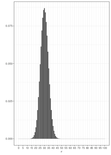
We can also use the built-in command rbinom to simulate values from a given Binomial distribution. For example, the following code can be used to produce the graph in Figure 2.2 that illustrates a histogram from a random sample of 10000 observations from a Binomial(0.25,33) distribution.

tibble(r=rbinom(n=10000,size=33,prob=0.25)) %>% 
  ggplot(aes(r)) + geom_histogram(
    breaks=seq(0,33),color="black",fill="grey"
  ) + theme_bw() + xlab("Number of successes") + 
  ylab("Absolute frequency") + 
  scale_x_continuous(breaks = seq(0, 33, 1), lim = c(0, 33))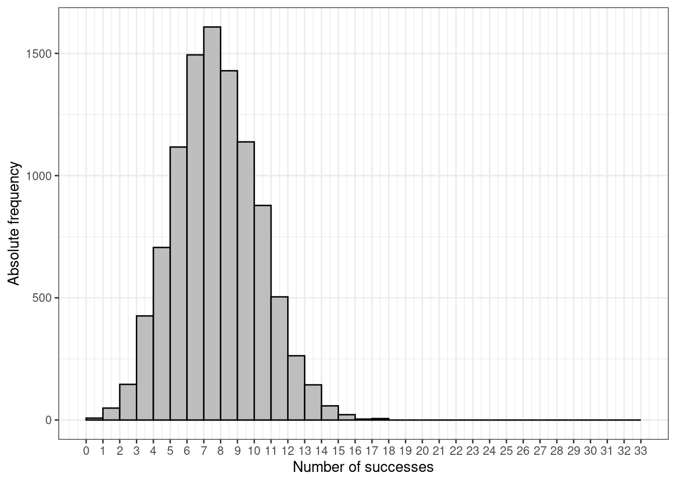

Figure 2.2: Histogram of a random sample of 10000 observations from a Binomial(\(\theta=0.25,n=33)\) distribution

The R code here is probably unnecessarily complicated to show some of the features in terms of customisation of the graph, using the tidyverse and ggplot2 approach. We first define a tibble, a special R object containing data, which we fill with a vector r that contains 10000 simulated values from the relevant Binomial distribution. We then apply ggplot to construct and style the histogram.

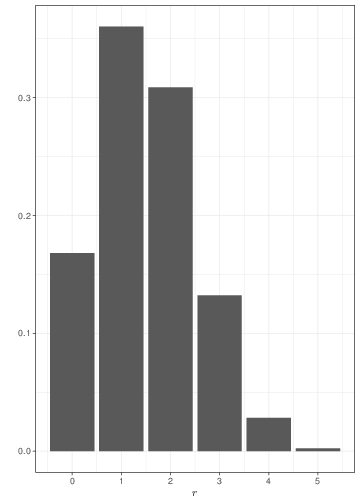
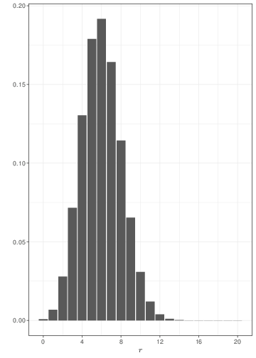
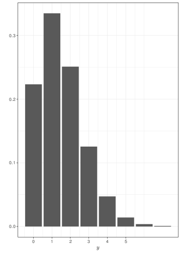
The graph in Figure 2.3 shows three examples of Binomial distributions with \(\theta=0.3\) but upon varying the sample size. As the sample size increases, the histogram becomes more symmetrical around the mean \((\theta=0.3)\).

Because of the mathematical definition of the Binomial distribution, it can be proved that if \(R\sim\mbox{Binomial}(\theta,n)\), then

The mean (or “expected value”) is \(\mbox{E}[R]=\mu=n\theta\);
The variance is \(\mbox{Var}[R]=\sigma^2=n\theta(1-\theta)\).

Consequently, for a single Bernoulli variable, the mean is simply \(\theta\) and the variance is simply \(\theta(1-\theta)\). Both the Bernoulli and Binomial distributions were derived by the Swiss mathematician Jacob Bernoulli, in the late 17th century. Bernoulli was part of a large family of academics and mathematicians, who have contributed to much of the early development of probability calculus and statistics.

2.2 Poisson

Suppose there are a large number of opportunities for an event to occur, but the chance of any particular event occurring is very low. Then the total number of events occurring may often be represented by a discrete variable \(Y\). The sampling process that can be used to describe this situation is based on the Poisson distribution, named after the French mathematician Siméon Denis Poisson. Poisson used this model in the 19th century in his “Research on the Probability of Judgments in Criminal and Civil Matters”, in which he modelled the number of wrongful convictions.

Mathematically, if \(y \sim \mbox{Poisson}(\theta)\) then we have that \[ p(y\mid\theta)= \frac{ \theta^y \; e^{-\theta}}{y!} \qquad y = 0,1,2,3,\dots \tag{2.3}\]

For a Poisson distribution, the parameter \(\theta\) represents both the mean and the variance: \(\mbox{E}[Y]=\mu=\mbox{Var}[Y]=\sigma^2=\theta\). This may at times be a limitation because often empirical data tend to violate this assumption — they show larger variance than the mean, a phenomenon often referred to as overdispersion. Suitable models can be used to expand the standard Poisson set up to account for this feature. In addition, in many applications, the Poisson sampling distribution will arise as a total number of events occurring in a period of time \(T\), where the events occur at an unknown rate \(\lambda\) per unit of time, in which case the expected value for \(Y\) is \(\theta = \lambda T\).

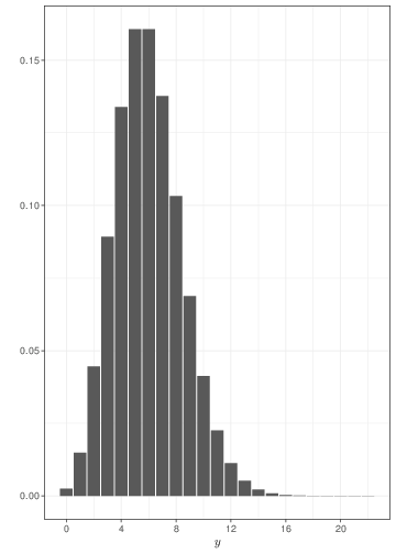
Generally speaking, the Poisson distribution is used to model sampling variability in observed counts, e.g. the number of cases of an observed disease in a given area. The examples in Figure 2.4 show that if events happen with a constant rate, observing for longer periods of time leads to smaller relative variability and a tendency towards a symmetrical shape. Comparison of Figure 2.4 with Figure 2.3 shows that, when sample size increases, a Binomial might be approximated by a Poisson with the same mean.

The main distinction between the Poisson and the Binomial models is that in the latter case we consider the number of events out of a fixed and known total number of possible occurrencies (the sample size, \(n\)). In the case of the Poisson, we generally consider the overall number of events (counts), without formally restricting the total number of occurrencies. For this reason, the Poisson distribution may be used to model the probability of observing a certain number of goals in a football match (which, theoretically is unbounded), while the Binomial distribution can be used to model the number of Gold medals won by Italy at the next Olympic Games (which physically is bounded by the total number of sporting events).

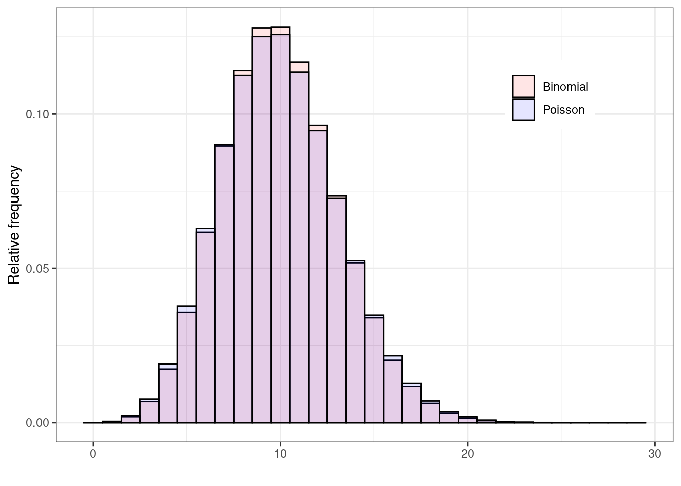
If you consider this, it becomes perhaps more intuitive why the Poisson is the limiting distribution for the Binomial, as \(n\) increases to \(\infty\). Figure 2.5 shows two histograms summarising 1,000,000 simulations from: a) \(y_1\sim\mbox{Binomial}(\theta=0.05, n=200)\); and b) \(y_2\sim\mbox{Poisson}(\mu=n\theta=7.5)\). As is possible to see, because the underlying probability \(\theta\) is fairly small (i.e. the event of interest is rare), for all intents and purposes, \(n=200\) is effectively as large as \(n\rightarrow\infty\) and the two distributions overlap almost completely. If \(\theta\) is larger, then we need a much bigger sample size \(n\) before the Binomial distribution is fully approximated by a \(\mbox{Poisson}(\lambda=n\theta)\).

Figure 2.5: Histogram for two samples of 1000000 observations from a Binomial(0.05,200) (in red) and a Poisson(7.5=0.05 \(\times\) 200) (in blue). When the two histograms overlap, the resulting colour is shaded to purple

We can use R to compute probabilities or simulate random numbers from a Poisson distribution in a similar fashion as to what shown above. For instance, if we set \(\theta=2\) we can compute the probability of observing \(y=8\) events using the following command (note that, somewhat confusingly, R calls the parameter we have indicated as \(\theta\) with the name lambda).

dpois(x=8,lambda=2)

[1] 0.0008592716

The answer could be determined also by a simulation approach, as follows.

set.seed(10230)
# Vector of number of simulations
n=c(100,1000,10000,100000,1000000,10000000)
# Initialise (an empty) vector of (numeric) probabilities 
prob=numeric()
# Simulates n[i] observations from a Poisson(lambda=2) and then 
# counts the proportion of simulations with value 8
for (i in 1:length(n)) {
   y=rpois(n=n[i],lambda=2)
   prob[i]=sum(y==8)/n[i]
}
# Formats and shows the output
nlab=format(n,scientific=FALSE,big.mark=",")
names(prob)=nlab
prob

       100      1,000     10,000    100,000  1,000,000 10,000,000 
 0.0000000  0.0000000  0.0015000  0.0008100  0.0007820  0.0008638

If we inspect the output of this process, we see that as we increase the size of the simulation to 10,000,000, then the numerical answer (0.0008638) becomes very close to the analytic one (0.0008593). When we consider a small number of simulations, our numerical estimate of the “true” analytic value is not very precise at all.

This process of numerical approximation of a quantity through simulation is often termed Monte Carlo analysis (more on this in STAT0019, if you take it).

2.3 Normal

The Normal distribution is fundamental to much of statistical analysis. Often it is referred to as Gaussian, from the name of its inventor, the German mathematician Carl Friedrich Gauss, who in the late 18th century used it to describe “normally distributed errors”.

A continuous variable is associated with a Normal distribution if we can assume that the underlying sampling process has the following properties:

Symmetry: we expect to see most of the observations scattered around a central location, with “errors”, or deviation from the central location becoming increasingly smaller as we move further away.
Unboundness: we do not place any physical restriction on the size of the values that the variable can take on. Technically speaking, we say that the range of the variable is the set \((-\infty; \infty)\). Notice however that, in reality, we will never observe a variable to take on the value \(\infty\) and all our observations will in fact be finite values.

When we assume that a variable \(Y\) is well described by a Normal distribution, we then write \(Y\sim \mbox{Normal}(\mu,\sigma)\), with \[ p(y\mid \mu,\sigma) = \frac{1}{\sqrt{2\pi} \sigma} \exp\left(-\frac{1}{2}\frac{(y-\mu)^2}{\sigma^2} \right); \qquad -\infty < y < \infty. \tag{2.4}\] Equation 2.4 shows that the Normal distribution is characterised by two parameters: \(\mu\) is the population mean and \(\sigma\) is the population standard deviation (see Chapter 1). Mathematically, the function in Equation 2.4 is a probability density. This is due to the fact that the underlying variable is continous and, as such, it can take on any real number, e.g. -1.21131765366772, 2.32279253568801, -6.52670986118001, 25.5187887120438.

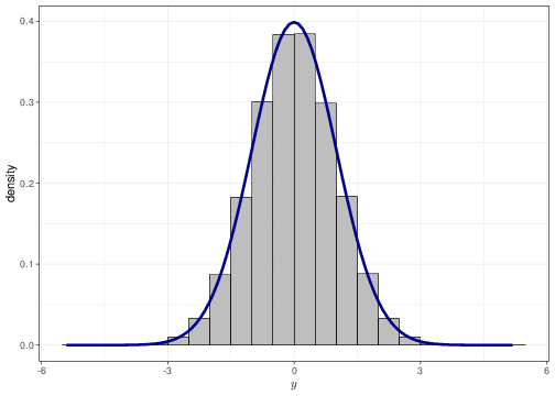
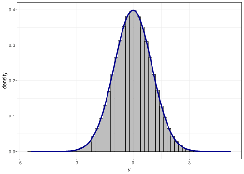
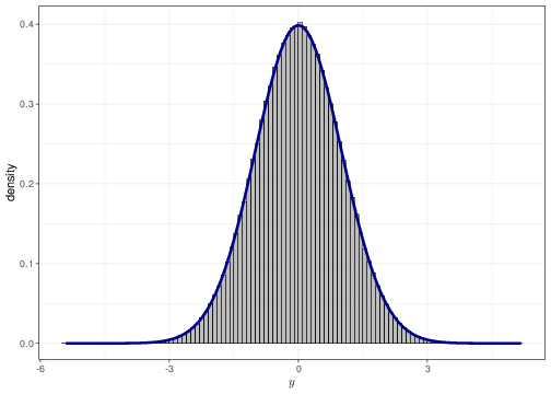
As mentioned in Chapter 1, for a continuous variable it is a mathematical impossibility that two different observations have the exact same value (technically, there is 0 probability that this happens). Thus, we can think of a probability density as a histogram where each group width is arbitrarily small. Figure 2.6 shows this for a sample of values from a Normal(0,1) distribution. The histogram in panel (a) uses group width of 0.50 — this means that the base on each rectangle is exactly 0.50 and the height is indicated along the \(y-\)axis of the graph. The histograms in panels (b)–(d) have increasingly small bar widths, approaching to a value \(\epsilon\rightarrow 0\). Each graph has superimposed a Normal(0,1) density — as is possible to see the graph in panel (d) shows essentially no distinction between the histogram approximation and the true density.

An important consequence is that, unlike the case of discrete variables, for which R commands such as dbinom(...) or dpois(...) allows us to calculate the actual probability of observing an exact value, for continuous variables the command dnorm(...) computes the density associated with a small interval around the value.

The Normal distribution (and the respective R code) can be used to compute tail area probabilities. For example, the command

qnorm(p=0.975,mean=0,sd=1)

[1] 1.959964

returns the value \(y\) such that for a variable \(Y\sim\mbox{Normal}(\mu=0, \sigma=1)\), we obtain \(\Pr(Y\leq y)=0.975\) — that is the 97.5% quantile of the Normal distribution. Figure 2.7 shows graphically that the area under the Normal(0,1) density between \(-\infty\) and 1.959964 \(\approx\) 1.96 does cover most of the probability mass — and in fact exactly 97.5%, which in turns implies that \(\Pr(Y>1.96)=0.25\).

Tail area probabilities can be used to compute the probability that a Normal variable lies within a given range. For example, we could use the following code

# Computes y1 so that, given Y~Normal(0,1), Pr(Y<=y1)=0.975
y1=qnorm(p=0.975,mean=0,sd=1)
# Computes y2 so that, given Y~Normal(0,1), Pr(Y<=y1)=0.025
y2=qnorm(p=0.025,mean=0,sd=1)
# Now verifies that Pr(Y<=y1) - Pr(Y<=y2) = 0.975 - 0.025 = 0.95
pnorm(q=y1,mean=0,sd=1)-pnorm(q=y2,mean=0,sd=1)

[1] 0.95

to check that the area comprised between the 97.5%-quantile and the 2.5%-quantile (i.e. the interval -1.96 to 1.96) does contain 95% of the probability distribution. Note the use of the built-in R functions qnorm and pnorm that compute the quantile, given a specified probability or a probability, given a specified quantile, under a Normal distribution.

2.4 Student’s t

A standardized Student’s t distribution has a prominent role in classical statistics as the sampling distribution of a sample mean divided by its estimated standard error. \(Y \sim \mbox{t}(\mu,\sigma^2,\nu)\) represents a Student’s \(t\) distribution with \(\nu\) degrees of freedom:

\[ p(y\mid \mu,\sigma^2,\nu) = \frac{\Gamma\left(\frac{\nu +1}{2}\right)}{\Gamma\left(\frac{\nu}{2}\right)\sqrt{\pi \nu}\sigma} \; \frac{1}{\left( 1+ \frac{(y - \mu)^2}{\nu \sigma^2} \right)^\frac{\nu +1}{2} }; \qquad -\infty < y < \infty, \tag{2.5}\] where the symbol \(\Gamma(x)=(x-1)!=(x-1)(x-2)\cdots1\) indicates the Gamma function (NB: not to be confused with the Gamma distribution presented in Section 2.5!).

For a Student’s t distribution, we can prove that

\(\mbox{E}[Y]= \mu\);
\(\mbox{Var}[Y]= \displaystyle\sigma^2\frac{\nu}{\nu-2}\).

Because of the mathematical format of the Student’s t distribution, it can be proved that the mean only exists if \(\nu>1\), and the variance only exists if \(\nu>2\).

The Student’s t distribution was invented by William Sealy Gosset, who published a paper with its derivation in 1908 under the pseudonym of “Student”, while being in secondment from his normal job at the Guinness brewery in Dublin, in the Department of Statistical Science at UCL. His work concerned the modelling of sampling variability for continuous, symmetric variables. He started by using a Normal model. However, because his problem involved samples of small sizes (for example, the chemical properties of barley where sample sizes might be as few as 3), this was not robust, i.e. it could not cope well with outliers, or extreme observations, which were still likely to be obtained, just because of sampling variability due to the small sample size.

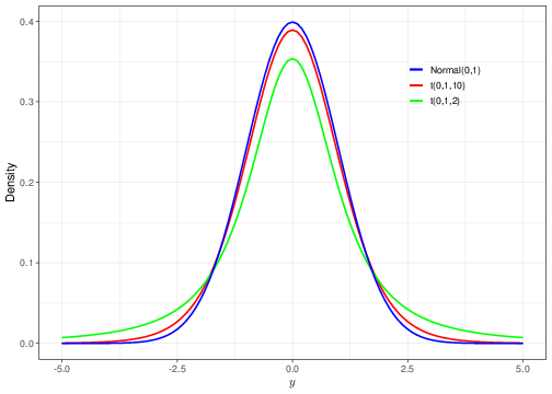
Figure 2.8: Comparison between different Student’s t and Normal distributions

The graph in Figure 2.8 shows the comparison between two Student’s t distributions (with \(\mu=0\) and \(\sigma=1\)) with degrees of freedom equal to \(\nu=10\) and \(\nu=2\), (in red and green, respectively), against a standard Normal distribution (again with \(\mu=0\) and \(\sigma=1\)).

As is possible to see, the lower the degrees of freedom, the “fatter” the tails of the Student’s t distribution, in comparison to the Normal. This implies that the Student’s t model assigns higher density to values that have larger deviations from the central tendency — this makes this model more “robust” to outliers or extreme observations. As \(\nu\rightarrow \infty\), the Student’s t distribution quickly converges to the standard Normal (note that \(\nu=10\) is already producing a pretty good level of overlap between the red and blue curves).

It is possible to use R to sample values from the Student’s t distribution. For example, we can create a graph similar to that of Figure 2.8 by typing the following command.

# Defines the range of the x-axis from -5 to 5 with increments of 0.01, 
# i.e. -5.00, -4.99, -4.98,..., 4.97, 4.98, 4.99, 5.00
# Plots the density of a t(0,1,3) distribution (in R, the default is 
# to assume mean=0 and var=1)
tibble(x=seq(-5,5,.01)) %>% ggplot(aes(x)) + 
  stat_function(
    fun=dt,args=list(df=3),lwd=1.1)
  )

Other built-in functions such as rt(...), pt(...) and qt(...) ara also available and can be used — more on this in Chapter 4.

2.5 Gamma and related distributions

Gamma distributions form a flexible and mathematically convenient class for continuous quantities constrained to be positive. Then \(Y \sim \mbox{Gamma}(a,b)\) represents a Gamma distribution with properties:
\[ p(y\mid a, b) = \frac{ b^a }{\Gamma(a) } y^{a-1} \; e^{-by}; \qquad -\infty < y < \infty; a,b>0 \tag{2.6}\] and \[\begin{eqnarray} \mbox{E}[Y] &= & \frac{a}{ b } \nonumber \\ \mbox{V}[Y] &= & \frac{a}{ b^2 } \nonumber \end{eqnarray}\]

The parameter \(a\) is called the shape, while \(b\) is called the rate of the Gamma distribution. Alternative parameterisations exist in terms of the parameters \((a,c)\), where \(c=1/b\) is called the scale — but note that, in this case, the form of the density in Equation 2.6 needs to be re-written accordingly!

One of the typical uses of the Gamma distribution is to model sampling variability in observed costs, associated with a sample of patients (you will see this extensively, if you take STAT0019). Other examples involve time-to-event models (e.g. to investigate how long before some event of interest occurs)

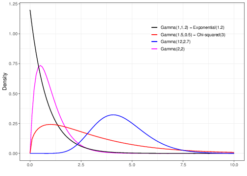
The general form of the Gamma distribution includes as special cases several other important distributions. Figure 2.9 shows a few examples of different Gamma distributions, upon varying the two parameters \(a\) and \(b\). As is possible to see, for specific choices of the parameters, we retrieve other distributions, related to the Gamma. Some important examples of such cases are discussed below.

Figure 2.9: Some examples of Gamma distributions upon varying the parameters \(a\) and \(b\). For different choices of the parameters, the Gamma distribution can give rise to other distributions, including the Exponential and the Chi-squared

2.5.1 Exponential

The Exponential distribution is obtained when we set \(a=1\), i.e. \[ Y\sim \mbox{Gamma}(1,b) \equiv \mbox{Exponential}(b). \tag{2.7}\] The Exponential distribution is sometimes used as model for sampling variability in times until an event of interest happens (e.g. time until a patient dies of a given disease). One major limitation of the Exponential model is however that it is only characterised by a single parameter \(b\), which also determines the value of the mean and variance as

\(\mbox{E}[Y]=\displaystyle\frac{1}{b}\);
\(\mbox{Var}[Y]=\displaystyle\frac{1}{b^2}\).

For this reason, the Exponential model is often too rigid and cannot represent well variations across a wide range of values for the variable \(y\).

2.5.2 Chi-squared

The Chi-squared distribution (sometimes indicated using the Greek letter notation \(\chi^2\)) is obtained from a Gamma distribution in which \(a=\nu/2\) and \(b=1/2\), i.e. \[ Y\sim \mbox{Gamma}\left(\frac{\nu}{2},\frac{1}{2}\right) \equiv \mbox{Chi-squared}(\nu). \tag{2.8}\] Using the properties of the Gamma distribution, it is trivial to derive that if \(Y\sim\mbox{Chi-squared}(\nu)\), then

\(\mbox{E}[Y]=\displaystyle\frac{\nu/2}{1/2}=\nu\);
\(\mbox{Var}[Y]=\displaystyle\frac{\nu/2}{1/2^2}=2\nu\).

A useful piece of distribution theory is that if \(Y_1,\ldots,Y_n \stackrel{iid}{\sim}\mbox{Normal}(\mu,\sigma^2)\) then the sample summaries are \[\begin{equation*} \bar{Y} = \frac{1}{n}\sum_{i=1}^n Y_i \quad \mbox{and} \quad S^2=\frac{1}{n-1}\sum_{i=1}^n (Y_i-\bar{Y})^2 \end{equation*}\] (recall Section 1.6) and it can be proved that \[ (n-1)\frac{S^2}{\sigma^2} \sim \mbox{Chi-squared}(n-1) \quad \mbox{and that} \quad \frac{(\bar{Y}-\mu)}{(S/\sqrt{n})} \sim \mbox{t}(0,1,n-1). \tag{2.9}\]

In addition, in a 1900 paper, Karl Pearson ¹ also proved that if \(Y_1,\ldots,Y_n\) are a set of observations and \(E_1,\ldots,E_n\) are the corresponding expected values from those observations (given a particular data generating process assumed to underlie the collection of the observations), then \[ \sum_{i=1}^n \frac{(Y_i-E_i)^2}{E_i} \sim \mbox{Chi-squared}(n-1). \tag{2.10}\]

We will use these results extensively in Chapter 4, in the context of hypothesis testing.

2.6 Other distributions

Probability calculus as taught in Statistical courses often concentrates on a small number of probability distributions, e.g. those mentioned above. But there are of course many more possibilities. Which distribution to use to reflect assumptions about the underlying data generating process and sampling variability (or indeed epistemic uncertainty about unobservable quantities — more on this in STAT0019) is a matter of substantive knowledge of the problem. And in reality, it becomes as much an art as it is a science, which requires experience as well as expertise.

Additional distributions that you are likely to encounter in STAT0014, STAT0015 and STAT0019 include the Uniform, log-Normal, Weibull, Gompertz, Beta, Multinomial, Dirichlet and Fisher’s F distributions. Good compendia of probability distributions are presented in several textbooks, including Spiegelhalter, Abrams, and Myles (2004) and Lunn et al. (2012)

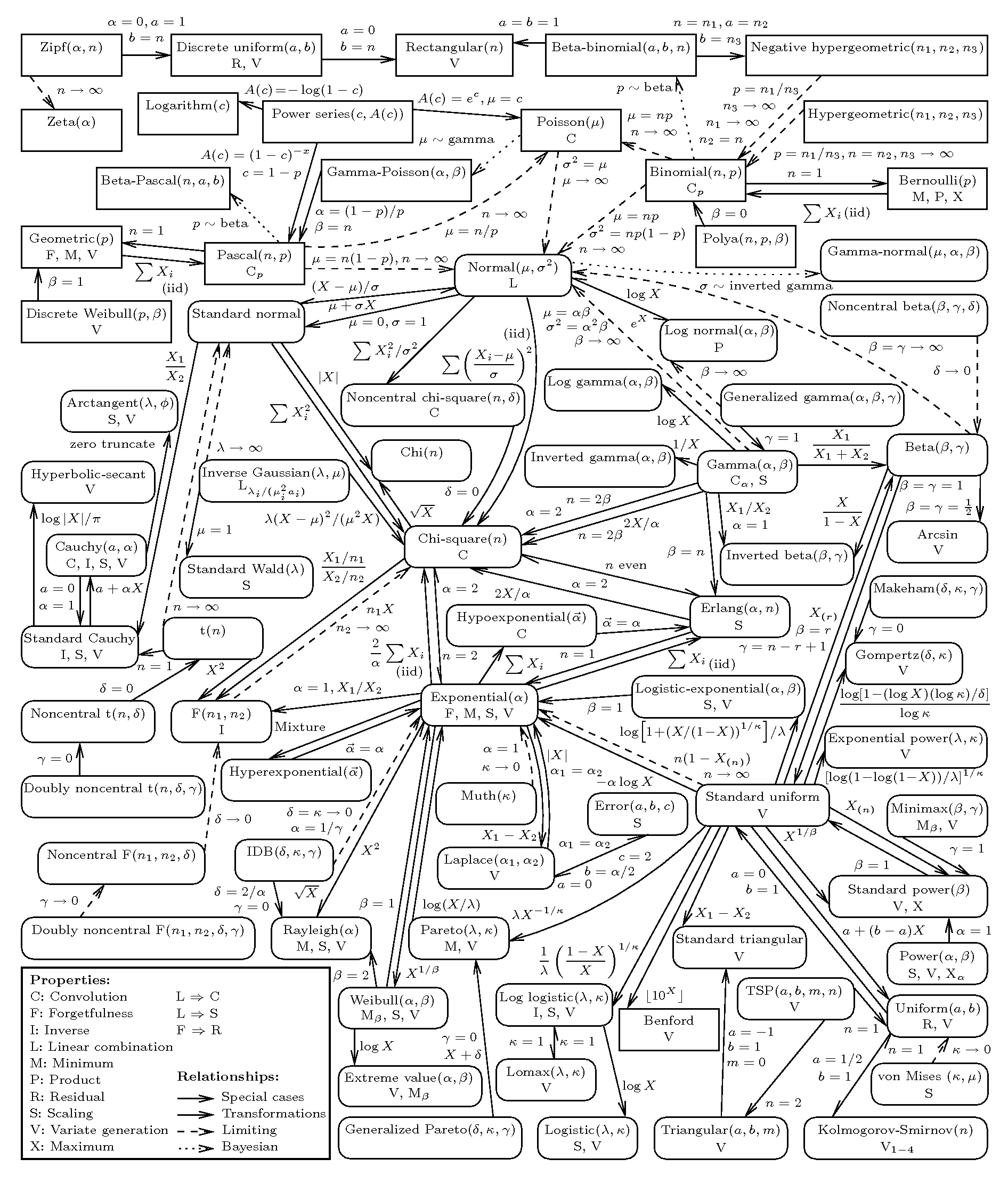
The graph in Figure 2.10 shows a graphical representation of the relationships among a large number of probability distributions. As is possible to see, there are many more choices than the simple few showed above. And interestingly, in many cases, the distributions tend to show close mathematical connections (for instance one distribution may be obtained as a special case of another, just like for the Exponential/Gamma). More details are given in Leemis and McQueston (2008).

Figure 2.10: A graphical representation of the relationships among a (non-exhaustive) set of univariate probability distributions. Source: Leemis and McQueston (2008).

Karl Pearson was a controversial figure. He was the founder of the Department of Applied Statistics (later renamed to Department of Statistical Science) at UCL in 1911, the first ever department of Statistics in any academic institutions. During his academic career, he has provided enormous and important contributions to the development of statistical theory and was widely regarded as the leading statistician in his time. However, he was sadly also a proponent of eugenics, a discipline that aimed at improving the genetic quality of a human population by excluding certain genetic groups judged to be inferior, and promoting other genetic groups judged to be superior. UCL has recently launched an inquiry into the history of eugenics at the university, which will also deliver recommendations on how to manage its current naming of spaces and buildings after prominent eugenicists.↩︎