3 Parameter estimation: doing Statistics

As mentioned earlier, in a nutshell the problem of statistical inference consists in

Obtaining a sample of observations $\boldsymbol{y}=(y_1,\ldots,y_n)$ from a population of interest. The process with which the data become observed is subject to sampling variability — you get to see only one of the many possible samples that could be obtained by extracting a number $n$ of units that is (typically) much smaller than the total size of the population $N$.
Characterise the sampling variability using a suitable probability distribution $p(\boldsymbol{y}\mid \boldsymbol\theta)$, defined as a function of a set of model parameters, $\boldsymbol\theta$, to describe the data generating process.
Use the observed data $\boldsymbol{y}=(y_1,\ldots,y_n)$ to learn about the unobservable population features described by the model parameters.

Interestingly (and somewhat confusingly) not even statisticians have agreed on a single way in which this process should be carried out. In fact, there are at least three main philosophical approaches to the problem of statistical inference.

3.1 Point estimates

3.1.1 The Bayesian approach

The Bayesian approach (which is the topic of STAT0019) is historically the first to have been developed. The original ideas and the basic structure date back to the publication of an essay by Reverend Thomas Bayes (Bayes 1763), an English non-conformist minister, after whom the whole approach is named.

A Bayesian model specifies a full probability distribution to describe uncertainty. This applies to data, which are subject to sampling variability, as well as to parameters (or hypotheses), which are typically unobservable and thus are subject to epistemic uncertainty (e.g. the experimenter’s imperfect knowledge about their value) and even future, yet unobserved realisations of the observable variables (Gelman et al. 2013).

As a consequence, probability is used in the Bayesian framework to assess any form of imperfect information or knowledge. Thus, before even seeing the data, the experimenter needs to identify a suitable probability distribution to describe the overall uncertainty about the data $\boldsymbol y$ and the parameters $\boldsymbol \theta$. We generally indicate this as $p(\boldsymbol y, \boldsymbol\theta)$. Using the basic rules of probability, it is always possible to factorise a joint distribution as the product of a marginal and a conditional distribution (you will see this again if you take STAT0019). For instance, we could re-write $p(\boldsymbol y,\boldsymbol\theta)$ as the product of the marginal distribution for the parameters $p(\boldsymbol \theta)$ and the conditional distribution for the data, given the parameters $p(\boldsymbol y\mid \boldsymbol\theta)$. But in exactly the same fashion, one could also re-express the joint distribution as the product of the marginal distribution for the data $p(\boldsymbol y)$ and the conditional distribution for the parameters given the data $p(\boldsymbol\theta\mid \boldsymbol y)$.

Consequently, \[ p(\boldsymbol{y},\boldsymbol{\theta})=p(\boldsymbol\theta)p(\boldsymbol{y}\mid\boldsymbol\theta) = p(\boldsymbol y)p(\boldsymbol\theta\mid \boldsymbol y) \] from which Bayes’ Theorem follows in a straightforward way: \[ p(\boldsymbol\theta\mid \boldsymbol y) = \frac{p(\boldsymbol\theta)p(\boldsymbol y\mid\boldsymbol\theta)}{p(\boldsymbol y)}. \tag{3.1}\] While mathematically incontrovertible, Bayes’ Theorem has deeper philosophical implications, which have led to heated debates, within and without the field of Statistics. In fact, the qualitative implications of this construction are that, if we are willing to describe our uncertainty on the parameters before seeing the current data through a probability distribution, then we can update this uncertainty by means of the evidence provided by the data into a posterior probability, the left hand side of Equation 3.1. This allows us to make inference in terms of direct probabilistic statements.

In all but trivial models, Equation 3.1 also presents some computational challenges because it is often very hard or even impossible to compute the ratio on the right hand side analytically. Consequently, until the 1990s the practical implementation of Bayesian models has been hampered by this problem. The widespread availability of cheap computing as well as the development of suitable clever methods for simulations (e.g. Markov Chain Monte Carlo, or MCMC, which you will encounter extensively if you take STAT0019) have helped overcome these problems and make Bayesian analysis very popular in several research areas, including economic evaluation of health care interventions and adaptive clinical trial designs.

Leaving all the technicalities aside (which you will encounter in more details if you take STAT0019), Bayesian inference proceeds by using the following scheme.

Define a “prior” distribution $p(\boldsymbol\theta)$ to describe the current uncertainty on the model parameters. This represents the knowledge before the data $\boldsymbol y$ become available.
Observe data $\boldsymbol y$, whose sampling variability is modelled using $p(\boldsymbol y\mid\boldsymbol\theta)$.
Apply (an approximation to the exact computation intrinsic in) Bayes’ Theorem of Equation 3.1 to compute the “posterior” distribution $p(\boldsymbol\theta\mid\boldsymbol y)$. This distribution represents the “revised” or “updated” level of uncertainty on the parameters $\boldsymbol\theta$, after the data $\boldsymbol y$ have become available.

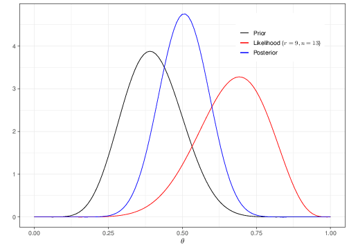
Suppose we consider a simple case where the data are $R\sim\mbox{Binomial}(\theta,n)$, with $n=13$ and we have observed $r=9$ successes. We want to make inference on the parameter $\theta$. Figure 3.1 shows an example of Bayesian inference in action (we will dispense with all the difficult technical points here and only concentrate on the interpretation).

Figure 3.1: An (extremely simplified!) example of Bayesian inference on a probability $\theta$ for a Binomial sampling distribution model, with $r=9$ observed successes out of $n=13$ individuals

Imagine that you are willing to specify the current level of uncertainty about $\theta$ using the black curve (labelled as “Prior”). This essentially implies that, before seeing any other data, you believe reasonable to assume that the most likely value for $\theta$ is around 0.4 and most likely it will be included in the interval (0.2 – 0.6). Values below 0.2 or above 0.6 are associated with increasingly smaller values of the probability mass as you move away from the mode (0.4) and towards the extremes (0 and 1). Technically, we could use a Beta(9.2,13.8) distribution to encode these assumptions (but, again, this is only a technicality and you will see more on this if you take STAT0019).

The red curve is a representation of the contribution brought by the observed data. In fact, this is the likelihood function (that is described in Section 3.1.2). Again, leaving all the details aside, the interpretation of the red curve is that, intuitively, because we have observed $r=9$ successes over $n=13$ individuals, the data seem to suggest that the “true” underlying probability of success may be higher than we originally thought (the red curve has a mode around 0.69231).

Finally, Bayesian inference is obtained by inspecting the blue curve, showing the posterior distribution. This is typically a compromise between the prior knowledge and the evidence provided by the data. As mentioned above, technically this can be complex, or even impossible to determine analytically — and in fact, most often we resort to simulation algorithms to obtain a suitable approximation.

In general, once the whole posterior distribution is available, it is then possible to describe it using suitable summaries For example, the usual point estimate is the mean of the posterior distribution. In the case of Figure 3.1, because the blue curve is reasonably symmetrical, the mean corresponds with the mode (the point where the distribution is highest), which in this case can be computed as 0.5056. So we initially thought that the probability that a random individual would experience the event under study was centered around the prior mean 0.4000 and we have revised this to the posterior summary 0.5056, after observing 9 individuals in a sample of 13 experiencing the event.

3.1.2 The Likelihood approach

This approach to statistical inference is almost single-handledly developed by Ronald Fisher ¹. The main ideas (which you will encounter extensively in STAT0015 and STAT0016) underlying Fisher’s theory can be somewhat roughly summarised as follows.

Unlike in the Bayesian approach, Fisher considers parameters as fixed (although unknown) quantities. As such, we cannot model our uncertainty over the true underlying value of $\theta$ using a probability distribution $p(\theta)$.
The only randomness in a statistical analysis is generated by the sampling variability associated with the observed data. We still want to use the data to learn about the world (as described by our model, indexed by the parameters $\boldsymbol\theta$) and to do so, the only thing we need to consider is the likelihood function.

Known, unknown, fixed…

Notice that in regards to point 1. above, also from the Bayesian point of view parameters may be fixed quantities: it is possible that the “true” proportion of males in the world is an unmutable constant — we just do not (and cannot!) know its true value with absolute certainty. The Bayesian way to deal with this epistemic uncertainty is to consider $\theta$ as a random variable and describe current uncertainty with the prior.

As shown in Chapter 2, we can model sampling variability using probability distributions. For example, in the case of the Binomial distribution, this is defined as \[\begin{eqnarray*} p(r \mid \theta, n) = \left( \begin{array}{c}n\\r\end{array} \right) \theta^r \; (1- \theta)^{n -r} \end{eqnarray*}\] — recall Equation 2.1. The expression above is a function of the observed data, given the values of the parameters (as should be clear from Chapter 2).

However, what we really want to do when making inference is not so much fixing the value for $\theta$ and computing probabilities for possible values of $r$ — rather we want to use the observed value of $r$ to learn what the most plausible value of $\theta$ is in the “true”, underlying DGP. Thus, Fisher’s main idea was to create a different kind of function, which varied with the parameters, but depended on the observed (fixed) $r$. He called this the likelihood function and defined it as the same equation used for the sampling variability associated with the model — except that the fixed and varying arguments are flipped around. For example, in the Binomial case, the likelihood function is \[ \mathcal{L}(\theta\mid r) = \theta^r(1-\theta)^{(n-r)}. \tag{3.2}\] Equation 3.2 only takes the terms in the Binomial sampling distribution that depend directly on the model parameter. For instance, the Binomial coefficient $\displaystyle \left( \begin{array}{c}n\\r\end{array} \right)$ is irrelevant because it does not include $\theta$ and thus it is discarded in forming the likelihood.

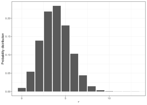
(a) Binomial sampling distribution $p(r\mid \theta=0.3)$

Panel (a) in Figure 3.2 shows the Binomial sampling distribution for a fixed value of $\theta=0.3$. If that was the “true”, underlying value of the probability that a random individual drawn from the population of interest experiences the event of interest, then we would expect 4 successes out of $n=13$ individuals sampled to be the most probable outcome. Observing 9 successes would be a somewhat unlikely event: we can use R to compute this probability as dbinom(x=9,size=13,prob=0.3)=0.00338.

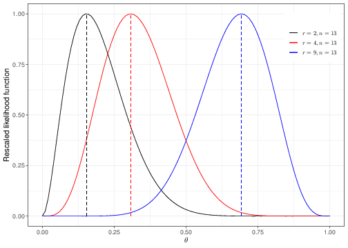
Panel (b) presents the likelihood function for three possible observed samples. The black curve corresponds to the analysis when $r=2,n=13$, the red curve is drawn for $r=4,n=13$ and the blue curve is derived in the case where $r=9$ and $n=13$ — notice that in the interest of comparability, we present here the rescaled likelihood functions, i.e. $\mathcal{L}(\theta\mid r)/\max\left[ \mathcal{L}(\theta\mid r) \right]$, so that the range on the $y-$axis goes from 0 to 1.

The interpretation of the likelihood function is that it describes “how likely” each possible value of the parameter is, given the observed data. For example, in the case of the black curve, the most likely value of the parameter after observing $r=2$ successes out of $n=13$ individuals is $\hat{\theta}=0.154$, which is indicated by the black dashed line. For $r=4$, then $\hat\theta=0.308$ (the red dashed line) and for $r=9$ then $\hat\theta=0.692$ (the blue dashed line).

Important

Notice that the language we have used here is purposedly pedantic and focuses on the concept of “how likely”, as opposed to “how probable”. This is because the likelihood function is not a probability distribution (technically, the reason for this is that the likelihood function does not integrate to 1, i.e. the area under the curve representing the likelihood function is not equal to 1, which is a necessary condition for a mathematical function to represent a probability distribution). Fisher was very clear on this — that is why he coined the phrasing “likelihood function”. But the concepts are sometimes conflated, so it is important to be careful on the distinction.

As seems sensible, the greater the number of observed successes, the higher the most likely value of the underlying true probability of success — if $\theta$ is indeed very large, then most people will experience the event and so we will tend to observe large values for $r$ in any given sample. So, by and large, the simplified process presented here describes how inference is performed in this setting:

we define a sampling distribution to describe variability in the observed data;
we turn this into a likelihood function for the model parameter(s); and
we determine the value that is associated with the highest likelihood (again: not probability!).

This is used as the best estimate — and it is referred to as the maximum likelihood estimator (MLE). Mathematically, this last step amounts to maximising the likelihood function. Technically this is done by finding the value for which the first derivatives of the function is equal to 0 and then checking that the second derivative of the function is negative to ensure that that point is indeed a maximum.

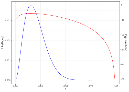
In order to perform this analytically (i.e. for a general value of the random variable $R$, rather than the specific observed value $r$), it is usually easier to work on the log scale, i.e. trying to maximise the log-likelihood $\ell(\theta)=\log\mathcal{L}(\theta\mid R)$. Figure 3.3 shows that both functions are maximised by the same point on the $x-$axis.

Figure 3.3: Likelihood function (in blue, with values on the $y-$axis on the left hand side) and Log-likelihood function (in red, with values on the $y-$axis on the right hand side) for the Binomial example with $r=2$. Both functions are maximised at the same point along the $x-$axis

Thus, if we consider the log-likelihood for the Binomial example, we have \[\begin{eqnarray*} \ell(\theta) = \log\mathcal{L}(\theta\mid R) = R\log\theta + (n-R)\log(1-\theta) \end{eqnarray*}\] and so, making use of the properties that: i. the derivative of a sum is the sum of the derivatives; ii. for a variable $x$, the derivative of $\log(x)$ is $\frac{1}{x}$; iii. for a variable $x$, the derivative of $\log(1-x)$ is $-\frac{1}{1-x}$; we can compute \[ \mbox{First derivative of $\ell(\theta)$} = \ell'(\theta)= \frac{R}{\theta} - \frac{n-R}{1-\theta}. \tag{3.3}\] Setting this to 0 and solving for $\theta$, i.e. finding the value $\hat\theta$ in correspondence of which the first derivative is 0, gives \[\begin{eqnarray*} \frac{R}{\hat\theta} - \frac{n-R}{1-\hat\theta} = 0 & \Rightarrow & (1-\hat\theta)R -\hat\theta (n-R) = 0 \\ & \Rightarrow & R-\hat\theta R -\hat\theta n + \hat\theta R = 0 \\ & \Rightarrow & \hat\theta = \frac{R}{n} = \sum_{i=1}^n \frac{Y_i}{n} = \bar{Y}, \end{eqnarray*}\] i.e. the sample mean of the $n$ individual Bernoulli variables (recall Section 2.1).

If we also compute the second derivative, i.e. the derivative of Equation 3.3 and check that it is negative (which in this case it is) to ensure that $\hat\theta$ is indeed a maximum point, then we have obtained a functional form for the MLE. And we can use this to compute its value for the observed sample, which in this case is $\displaystyle \hat{\theta}=\bar{y}=\frac{r}{n}=\frac{2}{13}=0.154$, which can be used as the point estimate for the parameter of interest.

In many cases the derivatives can be computed analytically, which means we can find the MLE as a function of the general random variable $R$ and then compute the value in correspondence of the observed value $r$, as in the case above. However, there may be cases where the resulting likelihood function is complex and either difficult or even impossible to differentiate (i.e. compute the derivatives). In these cases, most likely, you will be using a computer to maximise the likelihood function numerically. For example, R has several built-in functions to perform numerical optimisation, for instance optim or optimise, which can be used to that effect. The following code implements this calculation using optimise.

# Defines the likelihood function as a R function
Lik=function(theta,r,n) {
   # The function depends on three arguments:
   # 'theta' is a vector of values specifying the range of the parameter
   # 'r' is the observed number of successes 
   # 'n' is the observed sample size
   theta^r*(1-theta)^(n-r)
}
# Use 'optimise' to obtain the MLE for w=2 and n=13 in the interval (0,1), 
# ie the range of theta
optimise(Lik,r=2,n=13,interval=c(0,1),maximum=TRUE)

$maximum
[1] 0.1538463

$objective
[1] 0.003768044

Firstly, we code up the likelihood function of Equation 3.2 in the function Lik, which takes as arguments the parameter theta, as well as the observed data r and n. The we run optimise by passing as arguments the function we want to maximise (Lik), the values for the data (r and n), the interval over which we want to maximise the function (interval=c(0,1), which represents the range of $\theta$) and the option maximum=TRUE, which instructs R to compute the maximum (instead of the minimum of the function). The results is stored in the object maximum, which has a value of 0.1538463, which is essentially identical to the analytic value 0.1538462 (the differences are due to the approximation in the numerical optimisation procedure performed through optimise).

3.1.3 The Frequentist approach

The third major approach to statistical inference is termed frequentist and it was built on major contributions by Jerzy Neyman and Egon Pearson, in the 1930s².

As in the likelihood approach, parameters are considered to be unknown, but fixed quantities. However, the frequentist school does not attempt to make inference for a specific set of data, but rather it considers and evaluates inference procedures (e.g. the way in which an estimator is defined). Inference consists in the probabilistic assessment of the properties of the procedure, according to suitably defined criteria (more on this later).

In a nutshell, the frequentist approach defines a statistic, i.e. a function $f(Y)$ of the observed data, based on its “optimality” according to the long-run performance. In other words, we want to use as estimator for a given parameter a function of the observed data that, if we were able to repeat the experiment over and over under the same conditions would guarantee that, in the long-run, we would be certain of some properties.

Long-run/short-life

The “long-run” argument underpins the frequentist approach and all the theory developed by Neyman and Pearson. This was very popular at the time, although not universally advocated. And criticism of the frequentist philosophy was not confined to the field of Statistics. The British economist John Maynard Keynes is quoted to have dismissed it because “… in the long run, we are all dead” (Keynes 1923).

For instance, let us consider a Bernoulli sample of $n$ individuals $\boldsymbol{Y} = (Y_1,\ldots,Y_n)\stackrel{iid}{\sim}\mbox{Bernoulli}(\theta)$ and the two possible estimators \[f_1(\boldsymbol Y) = \sum_{i=1}^n\frac{Y_i}{n} = \bar{Y} \qquad \mbox{and}\qquad f_2(\boldsymbol Y) = \frac{\mbox{Med}(Y)}{n}.\] Here, $f_1(\boldsymbol Y)$ is the sample mean, where $f_2(\boldsymbol Y)$ is computed as the median of the data $\boldsymbol Y$ divided by the sample size $n$.

Now, imagine that we knew with no uncertainty that the true value of the underlying probability of success is $\theta=0.3$ — of course, in reality we cannot know this and to give our best estimate for its value is in fact the objective of the analysis. But if we did know, then we could imagine a simulation process that aims at mimicking would could happen if we were to repeat a very large number of times the experiment in which we collect data on $n=13$ individuals and record how many experience the event.

In R we could do this by using the following code

# Sets the 'seed' so that we always get the same results
set.seed(12)
# Sets the "true" value of the probability of success (assumed known)
theta=0.3
# Sets the sample size in each repeated experiment
n=13
# Sets the number of simulations
nsim=1000
# Defines a matrix "samples" with nsim rows and n columns, 
# initially with "NA" (empty) values
samples=matrix(NA,nsim,n)
# Then creates a loop to fill each row of the matrix "samples" with n 
# simulated values from a Binomial(theta, 1) (i.e. we simulate all the 
# individual Bernoulli data Y_i) 
for (i in 1:nrow(samples)) {
   samples[i,]=rbinom(n,1,theta)
}
head(samples)

     [,1] [,2] [,3] [,4] [,5] [,6] [,7] [,8] [,9] [,10] [,11] [,12] [,13]
[1,]    0    1    1    0    0    0    0    0    0     0     0     1     0
[2,]    0    0    0    0    0    0    0    0    1     0     1     0     0
[3,]    0    0    0    0    0    1    1    1    0     1     0     1     0
[4,]    0    0    0    1    0    1    0    0    0     0     1     0     0
[5,]    0    0    0    1    0    0    0    1    1     0     1     0     0
[6,]    0    0    1    0    1    0    1    0    0     0     1     1     1

(the command head(samples) shows the first few rows of the matrix of simulations, where 0 indicates that we have simulated a “failure” and 1 indicates a “success”).

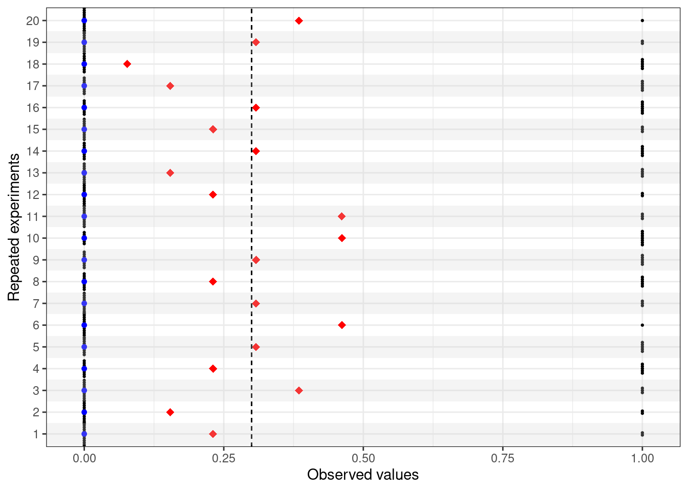
For each simulated dataset (=replicate of the experiment), we can record the observed value of the two statistics $f_1(\boldsymbol y)$ and $f_2(\boldsymbol y)$. Figure 3.4 shows the output for the first 20 replicates of the experiments: in each of the 20 rows in the graph, the black dots represent the $n=13$ simulated values (notice that, because we are simulating from a Bernoulli, then the only possible outcomes are 0=“failure” and 1=“success”); the red diamonds are the observed value of the sample mean $f_1(\boldsymbol y)$; and the blue squares are the observed values of the rescaled median $f_2(\boldsymbol y)$.

Figure 3.4: A graphical representation of a simulation exercise to describe repeated experiments from a Binomial case with $n=13$ and $\theta=0.3$. For each of the 20 simulations presented, the black dots indicate the simulated Bernoulli outcomes $y_1,\ldots,y_n$; the red diamonds indicate the sample means $\bar{y}$ and the blue dots are the rescaled sample medians $\displaystyle \frac{\mbox{Med}(\boldsymbol{y})}{n}$. The vertical dashed line indicates the true value for the parameter $\theta=0.3$

The frequentist approach makes use of the fact that, because they are functions of the observed data (which are subject to sampling variability), the statistics $f_1(\boldsymbol Y)$ and $f_2(\boldsymbol Y)$ also are subject to sampling variability — intuitively, this is expressed by the different values that we could observe for them, if we were able to do the experiment over and over again (as in Figure 3.4). Using the nsim simulations stored in the matrix sample, we could investigate the sampling distributions of $f_1(\boldsymbol Y)$ and $f_2(\boldsymbol Y)$, for example using the following commands

tibble(x=samples %>% apply(1,mean)) %>% 
  ggplot(aes(x)) + geom_histogram(bins=10,fill="grey",col="black") + 
  theme_bw() + xlab("") + ylab("Density") + 
  geom_segment(
    aes(x=0.3,y=-Inf,xend=0.3,yend=Inf),
    linetype="dashed",lwd=0.85
  ) 

tibble(x=samples %>% apply(1,median)/n) %>% 
  ggplot(aes(x)) + geom_histogram(bins=10,fill="grey",col="black") + 
  theme_bw() + xlab("") + ylab("Density")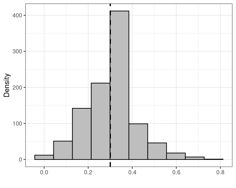

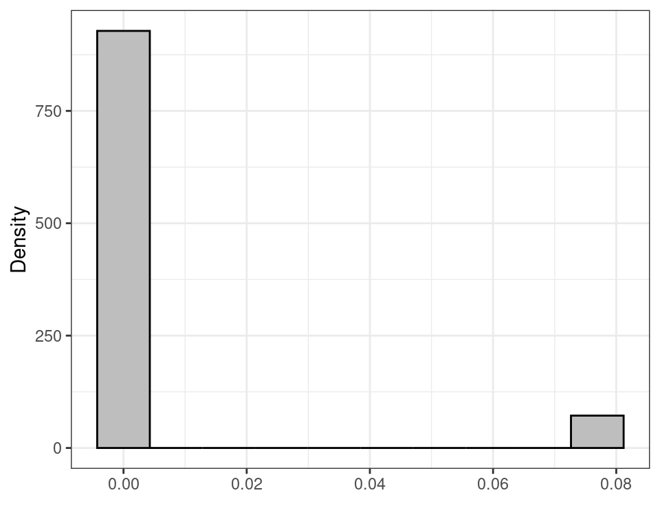
(the built-in function apply(matrix,1,FUN) takes all the rows of the first argument matrix and applies the function FUN to each of them, returning a vector of summaries, e.g. the mean or the median). Figure 3.5 shows histograms for the sampling distributions of $f_1(\boldsymbol Y)$ and $f_2(\boldsymbol Y)$, while Table 3.1 reports some summaries, including the mean, standard deviation, 2.5%, 50% (median) and 97.5% percentiles of the sampling distributions.

Table 3.1: Summary of the sampling distributions for the two statistics
	mean	sd	2.5%	median	97.5%
$\displaystyle f_1(\boldsymbol Y)=\bar{Y}$	0.3030	0.1316	0.0769	0.3077	0.6154
$\displaystyle f_2(\boldsymbol Y)=\mbox{Med}(\boldsymbol Y)/n$	0.0055	0.0199	0.0000	0.0000	0.0769

As is possible to see, the two estimators have rather different characteristics.

The rescaled sample median $f_2(\boldsymbol Y)$ has a much smaller standard deviation. However, this is only due the fact that its possible values are 0 or 0.0769 only and thus there is much less possible variation in the observed data, which leads to a smaller variance. If we consider the mean over the sampling distribution, the value is 0.00554, which is in fact very far from the true value $\theta=0.3$.
Conversely, the distribution of the sample mean $f_1(\boldsymbol Y)$ is centered around the “true” value for $\theta$. This is a very important property to a frequentist — it is called unbiasedness and a statistic having this property is called an unbiased estimator (for a given parameter). Formally, we define an unbiased estimator $f(\boldsymbol{Y})$ as one for which $\mbox{E}[f(\boldsymbol{Y})]=\theta.$

The reason why unbiasedness is so important to a frequentist is that it encapsulate perfectly the concept of long-run optimality: for any given sample, we have no reassurance that the unbiased statistic would give us a value equal, or even close, to the true underlying parameter. In fact, looking at Figure 3.4, none of the observed values for $f_1(\boldsymbol Y)$ is equal to the true value for $\theta=0.3$. However, because of its unbiasedness, we can say that in the log-run, on average we would “get it right” by using $f_1(\boldsymbol Y)$ to estimate $\theta$.

Unbiasedness (et al)

Unbiasedness is only one of the frequentist properties — arguably, the most compelling from a frequentist perspective and possibly one of the easiest to verify empirically (and, often, analytically).

There are however many others, including:

Bias-variance trade-off: we would consider as optimal an estimator with little (or no) bias; but we would also value ones with small variance (i.e. more precision in the estimate), So when choosing between two estimators, we may prefer one with very little bias and small variance to one that is unbiased but with large variance;
Consistency: we would like an estimator to become more and more precise and less and less biased as we collect more data (technically, when $n\rightarrow \infty$).
Efficiency: as the sample size increases indefinitely ($n\rightarrow\infty$), we expect an estimator to become increasingly precise (i.e. its variance to reduce to 0, in the limit).

3.1.4 You’re my one and only (theory)…?

Interestingly, as it happens, the MLE for a given parameter does generally have all the good frequentist properties. For this reason, we can effectively be frequentist and select the MLE as our optimal estimator, which has contributed to some people presenting and using these two approaches as a combined and unified theory. In fact, Fisher on the one hand and Neyman and Pearson on the other saw them as two irreconciliable schools of thought and have spent many years arguing vehemently with each other — so much so that when Fisher moved to UCL, a new special chair was created for him, to avoid him being in the same department as Pearson.³

What the two approaches do have in common, as mentioned above, is the fact that both take a non-Bayesian stance on how to deal with the model parameters. In both cases, parameters are considered as fixed but unknown quantities, which govern the DGP. In order to learn about the true, underlying value of the parameters, we can use suitable statistics: in the case of Fisher’s theory, the MLE because it is based on the likelihood function (which contains all the information that the sample can provide on the parameters); in the case of the frequentist approach, again most often the MLE, because it upholds all the good frequentist properties. But you should be aware of the fundamental distinction in these two approaches.

3.2 Interval estimation

We have just seen how different approaches to statistical inference produce point estimates for a parameter of interest. This is often a very good starting point — and sometimes it is the only summary reported, e.g. in non-scientific publications (such as in the mainstream media, as shown in Figure 3.6).

Figure 3.6: An example or inappropriate reporting of statistical quantities only as point estimates in the mainstream media

In reality, the point estimate is only likely to be indicative of what the true value of the underlying parameters could be — because of a combination of the sampling variability (that implies we can only learn so much from the observed data, unless $n\rightarrow \infty$, which it never is…) and the intrinsic epistemic uncertainty that we have on the parameter.

For this reason, it is a good idea to provide measures of interval estimate to complement the point estimate for a given (set of) parameter(s).

3.2.1 Bayesian approach

From a Bayesian point of view, in theory, interval estimate does not pose any additional complication. Once the full posterior probability distribution for the parameter has been computed, then we can simply present any summary we want. As seen in Section 3.1.1, the point estimate can be taken as the mean or the mode of the posterior. But we can also simply compute intervals that express directly probabilistic statements about the values of the parameters.

For example, we can prove that the posterior distribution for the Binomial example shown in Section 3.1.1 is a Beta$(18.2,17.8)$ — again the technical details are not important here and you will see them if you take STAT0019. We can use this information to compute analytically quantities such as the value $\theta_U$, the point in the parameter space (defined in this case as the interval $[0;1]$, because $\theta$ represents a probability) in correspondence of which $\Pr(\theta < \theta_U \mid y)=0.95$. With the current specification, this is 0.6408 — that is we can estimate that the posterior probability that $\theta$ is less than 0.6408 is exactly 95%.

Sometimes we will be able to make this or similar calculations analytically (which technically means we can solve an integral) and we can make this computations in R for instance using the command

q_U=qbeta(p=0.95,shape1=18.2,shape2=17.8)

which returns the exact value 0.640801.

A Bayesian interval is essentially computed using a similar process as the interval in correspondence of which a certain amount of probability lies: \[ \mbox{Bayesian 95\% interval} = [\theta_L; \theta_U] \mbox{ such that } \Pr(\theta_L \leq \theta \leq \theta_U \mid y) = 0.95. \]

Generally speaking we can use a simulation approach (which is essentially what MCMC does) and

Simulate a large number of values from the posterior distribution
Use the simulated values to compute tail-area probabilities and obtain the relevant interval.

For example, we can use the following R code to compute the 95% interval for the example above.

# Simulates 10000 values from the posterior distribution Beta(18.2,17.8)
theta=rbeta(n=10000,shape1=18.2,shape2=17.8)
# Computes the 2.5% quantile (that is the point leaving an area of 2.5% to its left)
q_L=quantile(theta,0.025)
# Computes the 97.5% quantile (that is the point leaving an area of 97.5% to its left)
q_U=quantile(theta,0.975)
# Displays the resulting interval estimate
c(q_L,q_U)

     2.5%     97.5% 
0.3436120 0.6679136

The result is that we compute that 95% of the posterior distribution lies in the interval $[0.344; 0.668]$, or, in other words, that the probability that the true parameter is contained between 0.344 and 0.668, given the model assumptions and the observed data is exactly 95%.

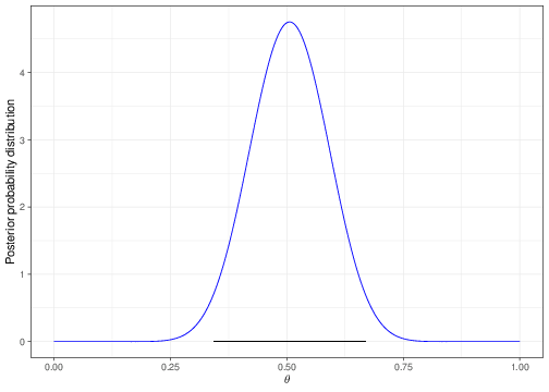
Figure 3.7: Posterior distribution for the Binomial example. The dark horizontal line below the distribution indicate the 95% interval estimate

Figure 3.7 shows again the posterior probability distribution; the dark horizontal line at the bottom of the histogram indicates the 95% interval.

Bayesian intervals

As mentioned above, theoretically, summarising the posterior distribution through an interval does not pose any additional problem, once the target distribution is available. The main problem is, of course, that we need to know what the posterior is before we can manipulate it — and this is the main point about doing simulations, e.g. using MCMC algorithms. This is not trivial, though and thus requires some specific training.

In addition, the procedure shown above to compute a Bayesian interval delivers what is often called a central interval — that is the one that leaves equal amount of area to its right and to its left. It does work very well if the underlying distribution is reasonably symmetric, but it may not be the best option when the distribution is skewed or “multimodal” (e.g. it has several “humps”, like a camel). In those cases, we can still compute suitable Bayesian intervals, based on slightly different theory and computations (these are often called “High Posterior Density”, or HPD intervals). The details are not important here.

3.2.2 Likelihood and frequentist approach

As mentioned in Section 3.1.2 and Section 3.1.3, the likelihood and frequentist approaches are not, in fact, a unified theory. Nevertheless, because effectively the MLE is often the “best” frequentist estimator, we can present the methodology in a compacted way.

The basic idea is that, as mentioned above, the MLE is a statistic, i.e. a function $f(Y)$ of the observed data and, as such, is associated with a sampling distribution. If we are able to determine what this sampling distribution is, then we can use it to compute tail-area probabilities that can be used to derive interval estimates.

For example, for a generic statistic $f(\boldsymbol Y)$, we can prove that \[ Z=\frac{f(\boldsymbol Y)-\mbox{E}[f(\boldsymbol Y)]}{\sqrt{\mbox{Var}[f(\boldsymbol Y)]}} \sim \mbox{Normal}(0,1), \tag{3.4}\] at least approximately, as the sample size $n\rightarrow \infty$ (which in practical terms, simply means that $n$ is “large enough”. A very general rule of thumb is that $n>30$ suffices for this result to hold).

We have seen before that the MLE for the probability of success $\theta$ in the $n$ independent Bernoulli case is the sample mean $\displaystyle f_1(\boldsymbol Y)=\bar{Y}=\sum_{i=1}^n\frac{Y_i}{n}=\frac{R}{n}$, where $Y_i \stackrel{iid}{\sim} \mbox{Bernoulli}(\theta)$. We can prove that the sampling distribution for $f_1(\boldsymbol Y)$ is approximately a Normal with mean $\theta$ (which makes $f_1(\boldsymbol Y)$ an unbiased estimator) and variance $\sigma^2/n$, where $\sigma^2=\theta(1-\theta)$. From this we can also derive that the standardised version of $f_1(\boldsymbol Y)$, obtained by considering $f_1(\boldsymbol Y)$ minus its expected value and divided by its standard deviation, is \[ \frac{\bar{Y}-\theta}{\sqrt{\theta(1-\theta)/n}} \sim \mbox{Normal}(0,1). \tag{3.5}\] We have seen in Figure 2.7 that for a Normal(0,1), the point 1.96 is the one leaving 97.5% of the distribution to its left. Similarly, we can prove that the point -1.96 leaves 2.5% to its left and thus the interval $[-1.96; 1.96]$ includes 95% of the probability \[\begin{equation*} \Pr\left(-1.96\leq \frac{\bar{Y}-\theta}{\sqrt{\theta(1-\theta)/n}} \leq 1.96 \right) \approx 0.95 \end{equation*}\] (the approximation comes about because: i. the distribution of $f_1(\boldsymbol Y)$ is only approximately Normal; and ii. we are using the rounded value 1.96 instead of the exact quantile of the Normal distribution). Re-arranging the terms inside the probability statement, we get \[ \Pr\left(\theta -1.96\sqrt{\frac{\theta(1-\theta)}{n}} \leq \bar{Y} \leq \theta + 1.96\sqrt{\frac{\theta(1-\theta)}{n}} \right) \approx 0.95. \tag{3.6}\]

At this point, we need a further layer of approximation: we do not know the true value of the parameter $\theta$ — only its estimate $\hat\theta$ (e.g. the MLE) and so we can compute the 95% confidence interval for the original statistic $\bar{Y}$ as \[ \left[\hat\theta -1.96\sqrt{\frac{\hat\theta(1-\hat\theta)}{n}}; \hat\theta + 1.96\sqrt{\frac{\hat\theta(1-\hat\theta)}{n}}\right]. \tag{3.7}\]

Probability of what?…

There is a subtle but crucial point in this argument. Equation 3.6 computes a probability. This probability however is computed with respect to the sampling distribution of the statistic — not the parameter $\theta$. From the frequentist/likelihood point of view, this is perfectly fine — in fact neither Neyman and Pearson, nor Fisher would want to compute a probability distribution directly for the model parameters. To them, the parameters are just fixed quantities and so cannot be associated with distributions. $\theta$ has a “true” value and so $\Pr(\theta=\mbox{true value})=1$ and $\Pr(\theta\neq \mbox{true value})=0$ — we just do not know what the true value is.

Again in line with the long-run philosphy, the interpretation of a confidence interval is that if we were able to replicate the experiment over and over again under the same conditions and each time we computed a confidence interval according to the procedure in Equation 3.7, then, in the long-run, the resulting interval would cover the true value of the unknown but fixed parameter 95% of the times. Figure 3.8 expands on Figure 3.4, by including the 95% intervals computed using Equation 3.7, depicted as the blue horizontal lines.

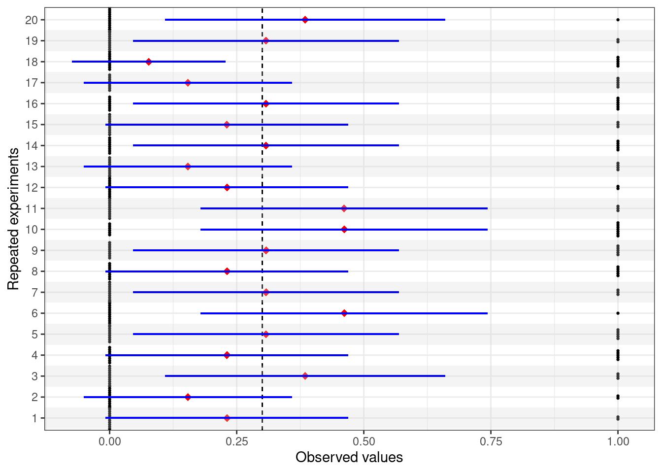
Figure 3.8: Graphical representation of the concept of confidence interval. The black dots are the simulated values for the observed Bernoulli data, in each of 20 replicates of the experiment. The red diamonds indicate the computed sample mean for each replicate. The dashed vertical line is drawn in correspondence of the “true” value of the parameter $\theta=0.3$. The blue lines indicate the 95% confidence intervals computed using the procedure described above.

For 19 out of the 20 potential replicates of the experiments presented in Figure 3.8, the procedure for computing the confidence interval succeeds in covering the true underlying value of $\theta=0.3$, shown as the dashed vertical line.

However, there is one potential replicate (experiment number 18) in which the procedure fails to cover the true value of the parameter. This is not entirely surprising: the procedure for the confidence interval “gets it right” 19/20 or 95% of the times.

And this is the meaning of the analysis based on the confidence interval: nothing to do to the uncertainty about the true value of the parameter — as mentioned above, there is no such thing in the frequentist paradigm. What we can evaluate is the long-run performance of the procedure.

In more general terms, building on Equation 3.4, considering a statistic $\hat\theta=f(\boldsymbol Y)$ used to estimate a parameter $\theta$ and with sampling distribution described (at least approximately) by a $\mbox{Normal}(\theta,\sigma^2/n)$, we can derive a form of the 95% confidence interval as \[ \left[\hat\theta -1.96 \frac{\sigma}{\sqrt{n}}; \hat\theta + 1.96 \frac{\sigma}{\sqrt{n}} \right]. \tag{3.8}\]

Confidence intervals

To be precise, the idea of confidence intervals as presented above is central to the purely frequentist approach — in fact the mathematical derivation is due to the work of Neyman, who wrote a landmark paper on this topic in 1937, drawing on the work he had done with Egon Pearson at UCL.

The mathematical formulation in purely likelihood terms derives the interval estimates in a fairly similar way, by considering the sampling distribution of the statistic $f(Y)$ (possibly approximated by a Normal distribution) and then computing the interval as \[ \left[\hat\theta -1.96 \frac{1}{\sqrt{-\ell{''}(\hat\theta)}}; \hat\theta + 1.96 \frac{1}{\sqrt{-\ell{''}(\hat\theta)}}\right], \] where $\ell{''}(\hat\theta)$ is the second derivative of the log-likelihood, evaluated at the MLE $\hat\theta$. The quantity $-\ell{''}(\theta)$ is often referred to as the observed Fisher’s Information.

For all intents and purposes, often the two procedures tend to return the same numerical value for the confidence interval.

Example 3.1 (Normal data; unknown mean, known variance) We now turn to a slightly more complex (but extremely useful and used) example. Consider data $y_1,\ldots,y_n\stackrel{iid}{\sim}\mbox{Normal}(\mu,\sigma^2)$, e.g. the following $n=30$ observations.

 [1]  -3.899644  70.906300  64.799692  48.582441  42.830802   2.448935
 [7]  18.350713   6.201232 -41.826326 -19.574827   7.668143   6.037137
[13]  58.216779  13.642063  25.834383  40.493779  19.744473  60.579431
[19]  22.770209  50.304467 -37.099194  14.960456   7.974603   3.912337
[25]  17.916688  87.621813  30.473627  10.823798  42.116799  13.358217

The parameters vector is thus $\boldsymbol\theta=(\mu,\sigma)$. However, imagine for now that we have full knowledge of the population standard deviation, e.g. $\sigma=32$. Thus, the only relevant parameter (for which we want to make point and interval estimation) is the population mean, $\mu$.

We can compute the MLE by considering the likelihood function. Recalling Equation 2.4, we can write the Normal sampling distribution for $n$ iid variables $\boldsymbol{Y} = (Y_1,\ldots,Y_n)$ as the product of the individual distributions for each $Y_i$ (this results comes about thanks to the assumption of independence), as \[\begin{eqnarray*} p(\boldsymbol{Y}\mid \mu,\sigma) & = &\prod_{i=1}^n p(Y_i\mid\mu,\sigma) = p(Y_1\mid\mu,\sigma)p(Y_2\mid\mu,\sigma)\cdots p(Y_n\mid\mu,\sigma) \\ & =& \frac{1}{(2\pi\sigma^2)^{n/2}} \exp\left(-\frac{1}{2}\sum_{i=1}^n\frac{(Y_i-\mu)^2}{\sigma^2} \right). \end{eqnarray*}\] Thus, the likelihood function for $\mu$, given $(\boldsymbol Y,\sigma)$ is \[ \mathcal{L}(\mu\mid \boldsymbol Y,\sigma) = \exp\left(-\sum_{i=1}^n(Y_i-\mu)^2\right), \tag{3.9}\] from which we can derive the log-likelihood \[ \ell(\mu) = \log\left(\exp\left(-\sum_{i=1}^n(Y_i-\mu)^2\right)\right) = -\sum_{i=1}^n(Y_i-\mu)^2.\]

Making use of the facts that: i. for a variable $x$ and a constant $a$, the derivative of $(a-x)^2$ is $-2(a-x)$; ii. the derivative of a sum is the sum of the derivatives; iii. $n\bar{Y}=\sum_{i=1}^n Y_i$; and iv. $\sum_{i=1}^n \mu=n\mu$,

we can compute the first derivative \[ \ell{'}(\mu) = -\left(-2\sum_{i=1}^n (Y_i-\mu)\right) = 2(n\bar{Y}-n\mu) = 2n(\bar{Y}-\mu). \tag{3.10}\]

Setting this to 0 and solving for $\mu$, we get \[\begin{eqnarray*} 2n(\bar{Y}-\mu) = 0 & \Rightarrow & 2n\bar{Y}=2n\mu \\ & \Rightarrow & \hat\mu = \bar{Y}. \end{eqnarray*}\] Once again, the MLE for the population mean is the sample mean $\bar{Y}$. Numerically, given the sample above, the MLE is $\bar{y}=22.872$.

In order to compute the 95% confidence interval around this point estimate, we can make use of simple probability calculus and prove that if $n$ variables $X_1,\ldots,X_n\stackrel{iid}{\sim}\mbox{Normal}(\mu,\sigma^2)$, then \[ \sum_{i=1}^n X_i = X_1 + \ldots + X_n \sim \mbox{Normal}(n\mu, n\sigma^2). \] In addition, we can prove that for any constant $a$, if $X\sim\mbox{Normal}(\mu,\sigma^2)$, then $aX \sim \mbox{Normal}(a\mu, a^2\sigma^2)$.

Putting these two results together implies that \[ \bar{Y} = \sum_{i=1}^n\frac{Y_i}{n} \sim\mbox{Normal}\left(\mu, \frac{\sigma^2}{n}\right), \tag{3.11}\] i.e. the sampling distribution of the sample mean is Normal with mean equal to the underlying population mean (which makes it unbiased) and variance equal to the population variance $\sigma^2$, rescaled by the sample size $n$. We have already used this results when computing the confidence interval for the Bernoulli case seen above.

In the present case, because we know that $\sigma=32$ and $n=30$ then $\sqrt{\frac{\sigma^2}{n}}=\sqrt{34.13}=5.84$ and thus $\bar{Y}\sim \mbox{Normal}(\mu,34.13)$. Consequently, using Equation 3.8, we can compute the 95% confidence interval as \[\begin{eqnarray*} \left[\bar{Y} -1.96 \frac{\sigma}{\sqrt{n}}; \bar{Y} +1.96 \frac{\sigma}{\sqrt{n}}\right] &=& [22.872-1.96(5.84); 22.872 +1.96 (5.84)] \\ & = & [11.42; 34.323]. \end{eqnarray*}\]

Example 3.2 (“Normal data; unknown mean and variance”) The case in Example 3.1 is obviously unrealistic: it is fairly difficult to imagine that we know with absolute certainty the value of a population parameter. More likely, we may observe data that we are willing to associate with some Normal sampling distribution, without knowing the underlying “true” value for $\boldsymbol \theta =(\mu,\sigma^2)$. We may still be mainly interested in point and interval estimates for the population mean $\mu$, but this time we consider the case where also the population variance $\sigma^2$ is unknown.

The first extra complexity is that now, when computing the likelihood function we have something that depends on 2 parameters: \[ \mathcal{L}(\mu,\sigma\mid \boldsymbol Y) = \sigma^{-n}\exp\left( -\frac{1}{2\sigma^2}\sum_{i=1}^n (Y_i-\mu)^2 \right). \] The log-likelihood is \[\begin{eqnarray*} \ell(\mu,\sigma) & = & \log\left( (\sigma^2)^{-n/2}\exp\left( -\frac{1}{2\sigma^2}\sum_{i=1}^n (Y_i-\mu)^2 \right) \right) \\ & = & -\frac{n}{2}\log\sigma^2 -\sum_{i=1}^n\frac{(Y_i-\mu)^2}{2\sigma^2} \end{eqnarray*}\] and we now need to compute two fist derivatives: one with respect to $\mu$ and the other with respect to $\sigma^2$. These are \[ \ell{'}(\mu) = \frac{2}{2\sigma^2}\sum_{i=1}^n(Y_i-\mu) \tag{3.12}\] \[ \ell{'}(\sigma^2) = -\frac{n}{2\sigma^2} + \sum_{i=1}^n\frac{(Y_i-\mu)^2}{2\sigma^4} . \tag{3.13}\] Equation 3.12 is basically identical to Equation 3.10 and so the computation of $\ell{'}(\mu)$ is similar to what shown in the case for know variance. As for Equation 3.13, we make use of the facts that: i. $\frac{1}{\sigma^n}=\sigma^{-n}=(\sigma^2)^{-n/2}$; ii. for a variable $x$, the first derivative of $\log x$ is $\frac{1}{x}$; iii. for function $f(x)$, the first derivative of $\frac{a}{f(x)}$ is the ratio $[af^{'}(x)]/f(x)^2$; and iv. the derivative of a sum is the sum of the derivatives.

Now, setting Equation 3.12 to 0 and solving for $\mu$ gives rise to \[ \hat\mu = \bar{Y}\] exactly as in the case for known variance of Example 3.1. Setting Equation 3.13 to 0 and solving for $\sigma^2$ gives \[\begin{eqnarray*} -\frac{n}{2\sigma^2} + \sum_{i=1}^n\frac{(Y_i-\mu)^2}{2\sigma^4} = 0 & \Rightarrow& -n\sigma^2 + \sum_{i=1}^n(Y_i-\mu)^2 = 0 \\ & \Rightarrow & \sigma^2 = \sum_{i=1}^n \frac{(Y_i-\mu)^2}{n}. \end{eqnarray*}\] Because we do not know the true value for $\mu$, in order to materially compute the MLE estimator $\hat\sigma^2$ of $\sigma^2$ we need to replace it with our best estimate, i.e. the MLE $\bar{Y}$ and so the MLE estimate for $\sigma^2$ is \[\hat\sigma^2 = \sum_{i=1}^n \frac{(Y_i-\bar{Y})^2}{n} \]

The crucial part of the procedure shown in Section 3.2.2 to compute the 95% confidence interval is given in Equation 3.4, which defines the sampling distribution for the statistic of interest. More specifically, for $f(\boldsymbol Y)=\bar{Y}$ as an estimator of the population mean $\mu$ (which is the case of interest here), then we can re-write \[ \frac{\bar{Y}-\mu}{\sigma/\sqrt{n}} \sim \mbox{Normal}(0,1), \] as seen in Example 3.1.

The only difficulty here is that in order to use the Normal(0,1) sampling distribution for $\bar{Y}$, we would need to know the true value of the other parameter $\sigma^2$. But we do not — the best we can do is to actually plug in an estimator. As seen above, the MLE is $\hat\sigma^2$. However, it can be proved that this is a biased estimator, i.e. $\mbox{E}[\hat\sigma^2] \neq \sigma^2.$ Conversely, we can prove that the estimator \[ S^2 = \frac{n}{n-1}\hat\sigma^2 = \sum_{i=1}^n \frac{(Y_i - \bar{Y})^2}{n-1} \tag{3.14}\] is unbiased and so, from a frequentist point of view, is preferred. This is one of the cases where the MLE is actually not optimal (at least from a purely frequentist point of view).

Using $S^2$ as the best proxy to the unknown (and actually unknown-able!) $\sigma^2$, we obtain the statistic \[ T=\frac{\bar{Y}-\mu}{S/\sqrt{n}}, \] which however is not associated with a standard Normal sampling distribution. However, expanding on Equation 2.9, we can derive the general result that \[ \frac{f(\boldsymbol Y)-\mbox{E}[f(\boldsymbol Y)]}{\sqrt{\hat{\mbox{Var}}[f(\boldsymbol Y)]}} \sim \mbox{t}(0,1,n-1), \tag{3.15}\] where $\hat{\mbox{Var}}[f(\boldsymbol Y)]$ indicates the “best” sample estimate of the underlying variance. Finally, we can use this result to derive the sampling distribution for $T$ \[\begin{equation*} \frac{\bar{Y}-\mu}{S/\sqrt{n}} \sim \mbox{t}(0,1,n-1). \end{equation*}\] Thus, to compute the confidence interval in this case we need to use tail-area probabilities from a $\mbox{t}(0,1,n-1)$ distribution — instead of the standard Normal we have used so far. Using R we can compute the quantiles of the $\mbox{t}(0,1,n-1)$ distribution as

which are numerically equal to $q_L=-2.045$ and $q_U=2.045$. Considering that the numerical value in the observed sample for $S^2$= is 897.2, we can then use these values to derive the 95% confidence interval for the sample mean as \[\begin{eqnarray*} \left[\bar{Y} -2.045\frac{S}{\sqrt{n}}; \bar{Y} + 2.045\frac{S}{\sqrt{n}}\right] & = & \left[ 22.872 -2.045(5.469); 22.872 + 2.045(5.469) \right] \\ & = & [11.69; 34.06]. \end{eqnarray*}\]

Warning

Notice that in this case, we happen to obtain data for which the sample variance $S^2$ is actually smaller than the true underlying value $\sigma^2$. Of course, in real life we would never know the true value of $\sigma^2$ and thus we could not make this assessment. And more importantly, we ought to use the t-version of the computation of the confidence interval, to account for the extra layer of uncertainty in the estimates.

Much as Karl Pearson, Fisher was also a very controversial figure. His brilliance as a scientist is undisputed and he has made contributions to many disciplines, including Statistics, Biology and Genetics. On the other hand, his views were also close to eugenics — in fact, he took the post of head of the Department of eugenics at UCL, in 1933. He was also heavily criticised for his views on the link between smoking and lung cancer, which he strongly denied in favour of some underlying genetic features, despite the evidence that was already at the time becoming substantial.↩︎
Jerzy Neyman (a Polish mathematician and statistician) and Egon Pearson (the son of Karl Pearson — see Section 2.5.2) developed most of the theory underlying the main frequentist ideas while the former was visiting the Department of Statistical Science at UCL, where the latter had taken over his father as head.↩︎
During his early career, Fisher had also heated arguments with Karl Pearson, whom he started off admiring very much, but with whom he fell out over a rejection of one of Fisher’s papers in Biometrika, the scientific journal edited by Karl Pearson.↩︎