SODF1: Estimating the Probability of meeting the USP<711> standard
Data description
The SODF1 USP monograph specifies a minimum % dissolution of Q=80% at 30min. The data consist of \(N_{lots}\) = 6 SODF1 lots made by a single manufacturer. Twelve units (tablets) from each lot were tested (total number of units \(N_{units}\) =72). Repeated measures of % dissolution were taken from each unit at 1, 2, 5, 10, 15, 20, and 30 minutes of dissolution time. Thus there were \(N\) = 6x12x7 = 504 total observations. The variables \(lot_n\) , \(unit_n\) , \(t_n\) , and \(y_n\) identify the unique lot (1 to 6), unique unit (1 to 72), dissolution time , and observed % dissolution, respectively, for each observation.
Model description
Some key assumptions of this model
Conditional independence of sampling and prior events (i.e., all “~”s are iid).
Homogeneity of error variance, \(\sigma^2\) as a function of time and mean % dissolution. This is an important assumption that is partially justified in this example. However, usually variance is lower near zero and 100% dissolution and higher near 50% dissolution.
Lot and unit (tablet) effects can be approximated as linear effects on the 3 underlying Weibull coefficients (\(M\), \(\log(T)\), and \(\log(b)\)).
Covariance of lot effects are negligible. Actually this assumption has little justification. however, with only 6 lots the covariances are not well determined. So we assume they are zero.
The dissolution profile of all units (tablets) can be adequately described by a 3-parameter Weibull model. The Weibull model does have a good success history. However, there are other models that may be appropriate in various applications.
Hierarchical likelihood sampling model
\({{y}_{n}}\overset{iid}{\mathop{\sim{\ }}}\,N\left( {{w}_{n}},{{\sigma }^{2}} \right)\)
\({{w}_{n}}={{\theta }_{1,uni{{t}_{n}}}}\cdot \left[ 1-\exp \left\{ {{\left( -\frac{{{t}_{n}}}{\exp \left( {{\theta }_{2,uni{{t}_{n}}}} \right)} \right)}^{\exp \left( {{\theta }_{3,uni{{t}_{n}}}} \right)}} \right\} \right]\)
\({{\left( \begin{matrix} M \\ \log \left( T \right) \\ \log \left( b \right) \\ \end{matrix} \right)}_{uni{{t}_{n}}}}={{\left( \begin{matrix} {{\theta }_{1}} \\ {{\theta }_{2}} \\ {{\theta }_{3}} \\ \end{matrix} \right)}_{uni{{t}_{n}}}}=\left( \begin{matrix} {{\mu }_{1}} \\ {{\mu }_{2}} \\ {{\mu }_{3}} \\ \end{matrix} \right)+{{\left( \begin{matrix} {{\varepsilon }_{1}} \\ {{\varepsilon }_{2}} \\ {{\varepsilon }_{3}} \\ \end{matrix} \right)}_{lo{{t}_{n}}}}+{{\left( \begin{matrix} {{\delta }_{1}} \\ {{\delta }_{2}} \\ {{\delta }_{3}} \\ \end{matrix} \right)}_{uni{{t}_{n}}}}\)
\({{\mathbf{\theta }}_{uni{{t}_{n}}}}=\mathbf{\mu }+{{\mathbf{\varepsilon }}_{lo{{t}_{n}}}}+{{\mathbf{\delta }}_{uni{{t}_{n}}}}\)
\({{\mathbf{\varepsilon }}_{i}}\sim MV{{N}_{3}}\left( \mathbf{0},\left[ \begin{matrix} {{\sigma }_{l,1}} & 0 & 0 \\ 0 & {{\sigma }_{l,2}} & 0 \\ 0 & 0 & {{\sigma }_{l,3}} \\ \end{matrix} \right] \right),i=1:{{N}_{lots}}\)
\({{\mathbf{\delta }}_{i}}\sim MV{{N}_{3}}\left( \mathbf{0},\Upsilon \right),i=1:{{N}_{units}}\)
\(\Upsilon =\left[ \begin{matrix} {{\sigma }_{u,1}} \\ {{\sigma }_{u,2}} \\ {{\sigma }_{u,3}} \\ \end{matrix} \right]\cdot \left[ \begin{matrix} 1 & {{C}_{12}} & {{C}_{13}} \\ {{C}_{12}} & 1 & {{C}_{23}} \\ {{C}_{13}} & {{C}_{23}} & 1 \\ \end{matrix} \right]\cdot \left[ \begin{matrix} {{\sigma }_{u,1}} & {{\sigma }_{u,2}} & {{\sigma }_{u,3}} \\ \end{matrix} \right]={{\mathbf{\sigma }}_{u}}\cdot \mathbf{\Omega }\cdot \mathbf{\sigma }_{u}^{T}\)
Prior model
Initially, more informative priors were employed, but these were gradually relaxed. The vague priors seemed to have little impact on the posterior estimates. Ultimately it was found that essentially “flat” priors gave essentially the same estimates as vague priors. It is possible that informative priors would be more approriate scientifically and also might lead to better convergence properties.
\(\sigma \sim \mbox{Uniform}\left( 0,+\infty \right)\)
\({{\mu }_{i}}\sim \mbox{Uniform}\left( -\infty ,+\infty \right),i=1:3\)
\({{\sigma }_{l,i}}\sim \mbox{Uniform}\left( 0,+\infty \right),i=1:3\)
\({{\sigma }_{u,i}}\sim \mbox{Uniform}\left( 0,+\infty \right),i=1:3\)
\(\mathbf{\Omega }\sim \mbox{LKJcor}\left( 1 \right)\)
Stan model code
The Code below may not be optimal, but seemed to produce fairly robust estimates in cases where the parameter values are well defined by the data. Notice that the vague priors have been commented out leading to the use of essentially “flat” priors.
The lot and unit latent effect estimates are not saved, although this might be desirable in some cases where the behavior of a particular lot under test is of interest. instead only the predicted mean % dissolution (\(w_n\)) is retained as a function of model parameters for comparison of predicted and observed.
Notice that the LKJcorr prior on \(\Omega\) is implemented using the Cholesky triangular decomposition matrix, \(L\).
# Create model for Stan
modelString = "
data {
int<lower=1> K;

int<lower=0> N;
int<lower=1> Nlots;
int<lower=1> Nunits;
int<lower=1,upper=Nlots> lot[N];
int<lower=1,upper=Nunits> unit[N];
vector[N] y;
vector[N] t;
}

transformed data {
vector[K] zero;
zero = rep_vector(0., K);
}
parameters {
real<lower=0> sigma;

cholesky_factor_corr[K] L;
vector<lower=0>[K] sigma_l;
vector<lower=0>[K] sigma_u;
vector[K] epsilon[Nlots];
vector[K] delta[Nunits];
vector[K] mu;
}

transformed parameters {
vector[N] w;
vector[K] theta;
matrix[K,K] Omega = L * L';
matrix[K,K] Upsilon = quad_form_diag(Omega, sigma_u);
for (n in 1:N){
  theta = mu + epsilon[lot[n]] + delta[unit[n]];
  w[n] = theta[1]*(1 - exp(-(t[n]/exp(theta[2]))^exp(theta[3])));
}
}

model {
// Priors - informative priors may improve convergence, e.g.,
//sigma ~ normal(0, 1);
//mu[1] ~ normal(100, 320);
//mu[2] ~ normal(0, 64);
//mu[3] ~ normal(0, 64);
//sigma_l ~ normal(0, 64);
//sigma_u ~ normal(0, 64);
L ~ lkj_corr_cholesky(1);

// Likelihood
for (i in 1:Nlots) epsilon[i] ~ normal(0, sigma_l);
delta ~ multi_normal_cholesky(zero, diag_pre_multiply(sigma_u,L));
y ~ normal(w, sigma);
}
" # close quote for modelString
MCMC execution time
The MCMC is set up to provide 16,000 draws from the posterior. This is done by setting iter=8000 and chains=4. Stan automatically drops the first half of each chain. This will take about 1h on a 4 core machine. It is recommended to modify the code on the first run to execute stan() and save the Stanfit to a RData file. Then in subsequent runs to simply re-read this file. This is to save having to re-run the MCMC each time if changes are needed later in the code. Actually 16,000 draws may be sufficient for estimation. the Chapter cites 80,000 draws which would take about 5-6 hours.
Posterior statistical summary
Notice that the effective sample sizes are quite small for some parameters (e.g., correlation parameters of unit effects or standard deviation parameters of lot effects). This is not surprising as these parameters are not well determined from the data. The model is likely somewhat over-determined. It is a good idea to examine tracings and distributions for acceptable convergence. I felt that convergence was adequate for this purpose. Estmates were relatively stable even with smaller MCMC samples.
[1] "TABLE 23.2 Marginal summary of model parameter joint posterior distribution for SODF1" mean se_mean sd 2.5% 50% 97.5% n_eff Rhat
sigma 1.5599621228 1.421187e-03 6.004001e-02 1.4458998006 1.559198e+00 1.681295e+00 1784.75614 1.007698
sigma_l[1] 2.1131520576 4.069931e-02 1.218355e+00 0.8658455803 1.813915e+00 5.141840e+00 896.13583 1.006112
sigma_l[2] 0.1113817786 3.047998e-03 8.423880e-02 0.0355901584 9.470732e-02 2.771359e-01 763.82691 1.003421
sigma_l[3] 0.0522789627 7.167612e-04 2.971282e-02 0.0193859724 4.568842e-02 1.242691e-01 1718.45731 1.002061
sigma_u[1] 0.2653856389 2.488940e-02 2.208517e-01 0.0170236232 2.102077e-01 8.072898e-01 78.73586 1.070555
sigma_u[2] 0.1451018948 2.767098e-04 1.355434e-02 0.1210784591 1.441923e-01 1.745401e-01 2399.42905 1.000713
sigma_u[3] 0.0455554149 1.965321e-04 7.188394e-03 0.0322695182 4.520173e-02 6.063004e-02 1337.81655 1.003765
Omega[1,1] 1.0000000000 NaN 0.000000e+00 1.0000000000 1.000000e+00 1.000000e+00 NaN NaN
Omega[1,2] 0.1656593406 2.685340e-02 4.781805e-01 -0.7996489905 2.121120e-01 9.134945e-01 317.09188 1.004216
Omega[1,3] -0.0107395660 3.430205e-02 4.882393e-01 -0.8783974801 -1.169547e-02 8.574156e-01 202.59341 1.015828
Omega[2,1] 0.1656593406 2.685340e-02 4.781805e-01 -0.7996489905 2.121120e-01 9.134945e-01 317.09188 1.004216
Omega[2,2] 1.0000000000 6.417387e-19 7.971948e-17 1.0000000000 1.000000e+00 1.000000e+00 15431.65432 0.999750
Omega[2,3] -0.2038815981 3.119607e-03 1.550840e-01 -0.4943624996 -2.069109e-01 1.088569e-01 2471.34920 1.001952
Omega[3,1] -0.0107395660 3.430205e-02 4.882393e-01 -0.8783974801 -1.169547e-02 8.574156e-01 202.59341 1.015828
Omega[3,2] -0.2038815981 3.119607e-03 1.550840e-01 -0.4943624996 -2.069109e-01 1.088569e-01 2471.34920 1.001952
Omega[3,3] 1.0000000000 6.347211e-19 7.070542e-17 1.0000000000 1.000000e+00 1.000000e+00 12409.07882 0.999750
mu[1] 95.4944701205 5.256912e-02 1.075245e+00 93.4439895098 9.547913e+01 9.762438e+01 418.36277 1.003729
mu[2] 2.3231321102 2.587934e-03 6.234708e-02 2.2191295471 2.324785e+00 2.424403e+00 580.39783 1.005578
mu[3] 0.2756780838 9.285587e-04 2.513526e-02 0.2280714359 2.759547e-01 3.241654e-01 732.73695 1.002264
Upsilon[1,1] 0.1192019664 1.520222e-02 1.971244e-01 0.0002898038 4.418727e-02 6.517168e-01 168.13816 1.036443
Upsilon[1,2] 0.0095156220 1.000032e-03 2.388702e-02 -0.0276119683 4.044271e-03 7.201751e-02 570.55348 1.014550
Upsilon[1,3] -0.0005042072 5.742474e-04 7.609445e-03 -0.0185350961 -5.023634e-05 1.394781e-02 175.59326 1.032934
Upsilon[2,1] 0.0095156220 1.000032e-03 2.388702e-02 -0.0276119683 4.044271e-03 7.201751e-02 570.55348 1.014550
Upsilon[2,2] 0.0212382686 8.172105e-05 4.016627e-03 0.0146599933 2.079141e-02 3.046426e-02 2415.76756 1.000704
Upsilon[2,3] -0.0013729863 2.283320e-05 1.124019e-03 -0.0037238370 -1.316922e-03 6.946628e-04 2423.33413 1.002318
Upsilon[3,1] -0.0005042072 5.742474e-04 7.609445e-03 -0.0185350961 -5.023634e-05 1.394781e-02 175.59326 1.032934
Upsilon[3,2] -0.0013729863 2.283320e-05 1.124019e-03 -0.0037238370 -1.316922e-03 6.946628e-04 2423.33413 1.002318
Upsilon[3,3] 0.0021269656 1.784291e-05 6.726166e-04 0.0010413218 2.043197e-03 3.676001e-03 1421.03236 1.003458Comparison of predicted and observed dissolution profiles
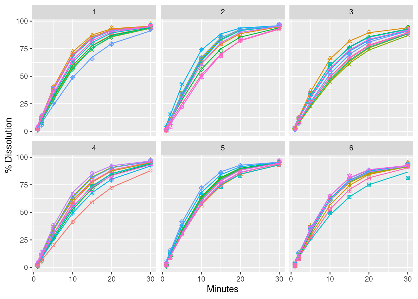
The figure in the chapter is missing some plot symbols. I corrected this below. The Weibull model appears to represent the profiles well. There are a few “outlier” values in the data visible in the plots.

Execution time for pass/fail prediction simulation
The simulation is currently set to generate 100 future USP<711> data sets for each MCMC draw. That would amount to 100*16000 = 1.6 million data sets to be analyzed by the USP<711> algorithm. That takes about 4min and results in a crude approximation. I recommend using npredata=800 which will take about half an hour of simulation time. Ideally more is better, but the added precision may not be worth it. in the end the estimated probabilities will be limited by the data, not the simulation I believe.
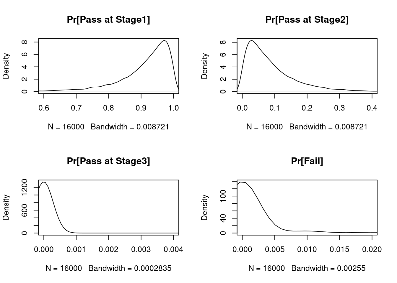
[1] "2022-09-23 16:26:47 BST"[1] "2022-09-23 16:29:04 BST"Posterior predictive distributions of USP <711> outcome probabilities

Quantiles of predictive distributions of USP <711> outcome probabilities
[1] "TABLE 23.3 Cumulative posterior predictive probabilities of USP<711> outcome events when testing SODF1. Based on 16000 simulated lots, each having 100 data sets per lot." 1pct 5pct 50pct 95pct 99pct
Pass at stage 1 0.59 0.74 0.93 0.99 1.00
Pass at stage 2 0.00 0.01 0.07 0.24 0.35
Pass at stage 3 0.00 0.00 0.00 0.00 0.01
Fail 0.00 0.00 0.00 0.01 0.09