library(BCEAweb)
BCEAweb()5 BCEAweb: a user-friendly web app to use BCEA
5.1 Introduction
In this chapter we introduce BCEAweb, a web interface for BCEA. BCEAweb is a web application aimed at everyone who does not use R to develop economic models and wants a user-friendly way to analyse both the assumptions and the results of an health economic evaluation. The results of any probabilistic model can be very easily imported into the web app, and the outcomes are analysed using a wide array of standardised functions. The chapter will introduce the use of the main functions of BCEAweb and how to use its capabilities to produce results summaries, tables and graphs.
The interface allows the user to produce a vast array of analysis outputs, both in tabular and graphical form, in a familiar environment such as a web page. The only inputs needed are the outputs of a probabilistic health economic model, be it frequentist (based for example on bootstrapping techniques) or fully Bayesian. It also includes functionalities to produce a full report and analyse the inputs of a probabilistic analysis to test the distributional assumptions.
Throughout this chapter, we will make use of the two examples used so far to show the functionalities of BCEA. The vaccine and smoking cessation models introduced in the previous chapters will be used as practical examples of how to use BCEAweb in real-world examples.
5.2 BCEAweb: a user-friendly web app to use BCEA
The vast majority of health economics models are built in MS Excel. This is because the users of these models are familiar with the software, and it is accepted by virtually all health authorities and decision makers across the world, including the National Institute for Health and Care Excellence (NICE), the Pharmaceutical Benefits Advisory Committee (PBAC) and the Canadian Agency for Drugs and Technologies in Health (CADTH). While models programmed in Excel are presented in a familiar, user-friendly fashion, the software itself can prove to be a limit when building complex models. The intricate wiring and referencing style of these models is often cause of programming errors. Very often models rely on Visual Basic for Applications (VBA) for Excel for complex procedures.
We acknowledge that Excel models are usually sufficient to demonstrate the value for money of new (or existing) technologies. However, often the presentation of the results is lacking, and the calculation of more complex quantities is inefficient (\(e.g.\) CEAC for multiple comparators) or are not feasible at all (\(e.g.\) EVPPI), mostly because VBA lacks the mathematical-statistical capabilities and flexibility of a language such as R. BCEAweb is aimed at researchers and analysts who would like to expand the scope of their health economic analyses without re-building models from scratch, programming additional analyses of the outputs and, perhaps most importantly, doing so without using R.
The main objective of BCEAweb is to make all the functionalities included in BCEA available and easy to use for everyone, without writing a single line of code. The program was inspired by the Sheffield Accelerated Value of Information (SAVI) web app (Strong et al., 2014), which can be accessed at the webpage (https://savi.shef.ac.uk/SAVI/). The focus of SAVI is the research on the methods of calculation of the expected value of (partial) information developed by Strong and colleagues (and presented in Section 4.3.3.2), and it also offers facilities to calculate cost-effectiveness summary measures. On the other hand, the purpose of BCEAweb is to offer an easy and standardised way to produce outputs from a health economic evaluation, with the EVPPI among them. It should also be noted that BCEAweb also includes an EVPPI calculation method which is faster than the one implemented in SAVI for multidimensional problems, based on the work on the EVPPI presented in (Heath et al., 2016).
The strength of BCEAweb is that it allows many different input formats, including csv files obtained from spreadsheet calculators (\(e.g.\) MS Excel), OpenBUGS/JAGS and R itself. The outputs can be saved either individually from the web app, or by exporting a modular summary in Word or pdf format, which also includes brief and flexible interpretations of the results. The report is modular, allowing users to choose the sections to be~included. Additionally, the plots may be generated using either of the three graphical engines in BCEA, that is the base R engine, ggplot2 and plotly.
5.2.1 A brief technical overview of BCEAweb
The web application BCEAweb is developed entirely in R-Shiny, a web application framework for R (Chang et al., 2015). Hart et al. (2025) consider the process of using R-Shiny as the future of HTA dissemination, with examples existing of a whole model being built on top of an R engine for computational efficiency and flexibility, but with the output visualised in a manner similar to a “standard” Microsoft Excel file, based on the web-based facilities of Shiny.
BCEAweb is available both online, at the web page (https://egon.stats.ucl.ac.uk/projects/BCEAweb/), or run locally via the BCEAweb R package, downloadable from https://github.com/giabaio/BCEAweb. BCEAweb connects the user to an R server so that the main functionalities of BCEA are quickly and easily available using a familiar web interface. This makes it possible to build an interactive application directly from R. A typical shiny application server is mainly based on two R scripts, the files ui.R and server.R. The first contains the code building the user interface, controlling the layout, objects and overall appearance of the web application, while the latter includes the logic, functions and R commands to be performed. These are managed server-side, producing a web page relying on HTML, CSS and Javascript without the programmer having to write in other languages than R. Additionally, the web app relies on additional files used in functions such as report generation.
On the client side, a modern web browser supporting Javascript is capable of displaying the web app. When accessing it through the internet, all the calculations are performed by the server, so that even the more demanding operations are not relying on the user’s device. The application can also be run locally, when a connection is not available or when potentially sensitive data cannot be shared on the internet, but obviously in this case the execution is performed on the users’ machine.
Any modern browser is able to display BCEAweb: both remotely, accessing it on the internet, and locally, by running it through R. The R package is needed only if running the web app locally, while an internet connection is required to access BCEAweb remotely.
5.2.2 Installing and running BCEAweb locally
As mentioned above, BCEAweb can also be run locally. To do so, R will be necessary as the local computer will act as both server and client. The package is available from both GitHub at https://github.com/giabaio/BCEAweb and R-universe at https://giabaio.r-universe.dev/BCEAweb. The GitHub version can be installed in R from source (requiring Rtools and compilation) using the devtools package, by executing the devtools::install_github("giabaio/BCEAweb") command. Otherwise, the install.packages('BCEAweb', repos = c("https://giabaio.r-universe.dev")) will download and install the binary package from R-universe, which will be faster by not requiring compilation.
Once the BCEAweb package is installed, the web application can be launched using the BCEAweb() function, which will open a new tab in the default web browser:
5.2.3 Running BCEAweb locally from inside of R
To run BCEAweb from within R, you can use the BCEAweb function, provided as part of the BCEAweb project on GitHub (https://github.com/n8thangreen/BCEAweb). This function launches the interactive interface in your default web browser on a local computer. Before using the function, ensure that the BCEA package is installed and loaded into your R session. To launch BCEAweb, simply call BCEAweb in your R console. You can optionally pass as arguments the simulation matrices for the effectiveness and cost, as well as a matrix with the simulations for all the relevant model parameters. By doing so, you don’t need to import these values manually from inside of the web app, streamlining the workflow.
5.2.4 Note on data import
As already mentioned, the output of an economic model can be imported easily, and in different formats, into BCEAweb. The functionalities of the web app require two different sets of inputs: the simulated (or sampled) values of the parameters, used to test the distributional assumptions of the PSA, and the PSA results, \(i.e.\) the costs and health effects resulting from each set of simulated (or sampled) parameter values, used to summarise and produce the results of the probabilistic analysis.
The latter set of values (\(i.e.\) the PSA results) is generally saved by all health economic models, as it represents the PSA results and is used to produce tools such as the cost-effectiveness plane. However, the sampled or simulated parameter values are not always saved in Excel models as they are usually discarded. Therefore, to make use of the tools to check the parametric distributional assumptions and to calculate the EVPPI and info-rank values, the analysts will need to make sure that the economic model will save the values of both the simulated parameter values and the PSA results. Details on how to format the inputs for the web app are reported in Section 5.2.6.1 and Section 5.2.7.
If the economic model outputs and/or the parameter inputs are available in the R workspace, these can be passed to the BCEAweb() function if the package is available offline. The model outputs should be provided as two separate objects, i.e., e and c, as matrices containing the model simulation of the effectiveness and cost variables, respectively. In both matrices, each row should represent a PSA simulation and columns the interventions considered in the model. The parameters argument can be used to provide all or a set of input parameters, with rows corresponding to the model output simulations in the e and c arguments, and with one column per parameters. Note the columns of the parameters matrix must be named.
For example, using the Vaccine example, the parameters can be passed to the function, so that they are available in the web application, as follows:
data(Vaccine)
BCEAweb(e = eff, c = cost, parameters = vaccine_mat)
5.2.5 Introduction to the interface
At a first look, BCEAweb seems to be a regular web page, and it actually is. The welcome page, first displayed when accessing the web app, is shown in Figure 5.1. This page provides details about what BCEAweb is, how to use it and about how it fits in the general process of a health economic evaluation. Many useful hyperlinks, coloured in orange, are included throughout the text. The tabs at the top of the page can be clicked to navigate through the different sections of BCEAweb.
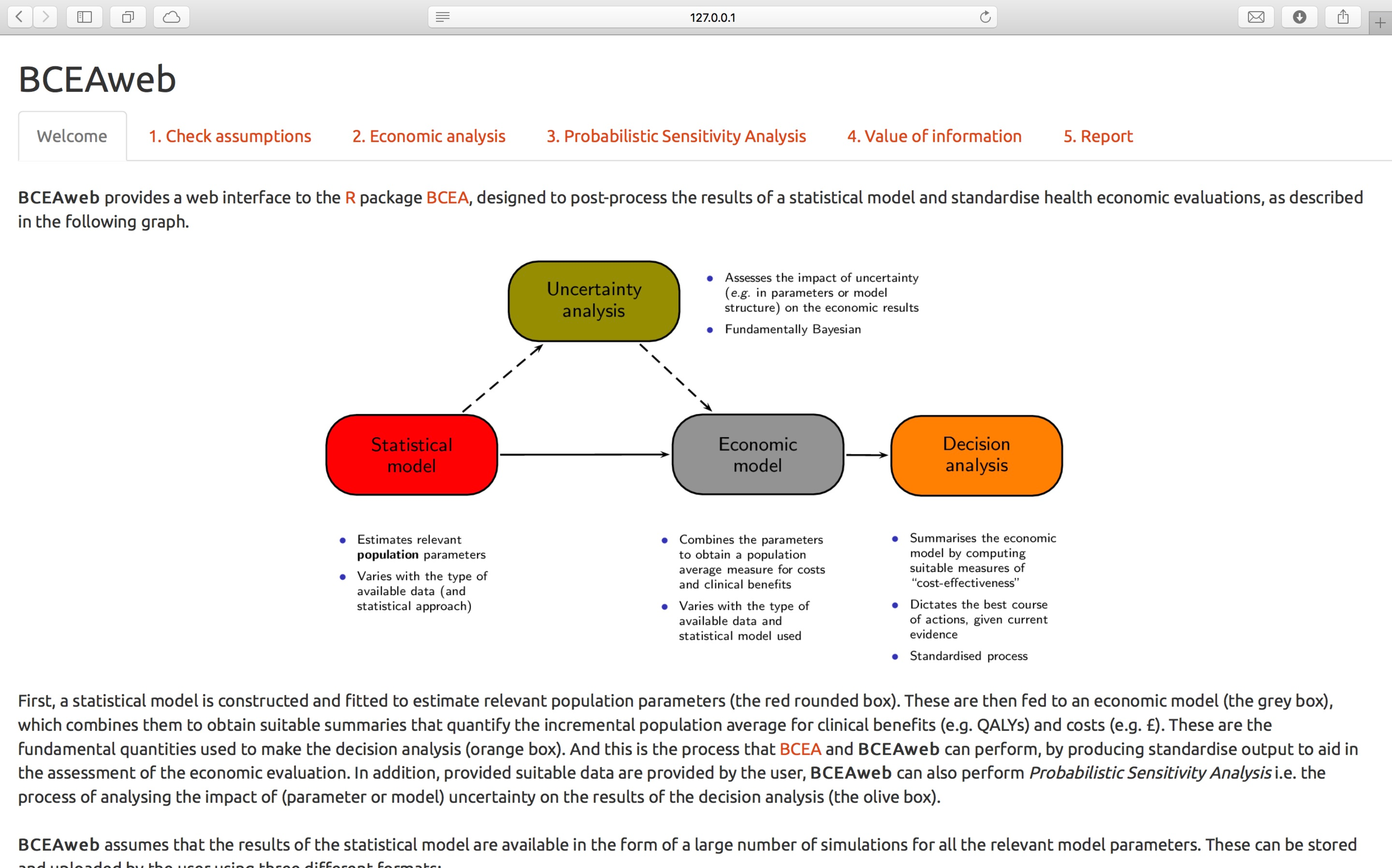
BCEAweb provides information on the web app and how to use it. The buttons at the top of the page are used to navigate through the pages. The web app is run locally in the examples pictured throughout this Chapter, and thus the address bar refers to the IP address localhost resolves to.
As shown in Figure 5.1, BCEAweb is fundamentally divided into 6 main pages. Each of them will be described in a section of this chapter. These can be easily accessed from any page by clicking on the respective label in the navigation bar:
Welcome: the landing page shown in Figure 5.1. The welcome page includes explanations about whatBCEAwebis and does, and provides a basic usage guide;Check assumptions: this page allows the users to check the distributional assumptions underpinning the probabilistic sensitivity analysis;Economic analysis: it is the place where the model outcomes are uploaded and the main settings regulated. It provides several tools for the analysis of the economic results. Shows the results on the cost-effectiveness plane and includes other analyses such as the EIB and the efficiency frontier;Probabilistic Sensitivity Analysis: calculates and shows results for tools commonly used in the probabilistic sensitivity analysis, \(i.e.\) as the pairwise and multiple-comparison CEAC and CEAF;Value of information: allows the calculation of the EVPI, EVPPI and the info-rank summary, based on the value of partial perfect information;Report: a standardised report, with modular sections, can be downloaded from this page.
5.2.6 Check assumptions
The first tab of the web app is called “Check Assumptions”. It is sufficient to click on its name in the navigation bar to access it. In this page, the user can upload the simulations of the parameters used in the iterations of the PSA from any probabilistic form of an economic model. The functionalities are particularly useful to easily test for violations of distributional assumptions, which might be caused for example by miscalculations of the distribution parameters in models caused by a very large number of inputs. Rather than checking the values one by one, the correctness of the sampled values can be analysed based on the analysis of the empirical (\(i.e.\) observed) distributions. This functionality extends BCEA and is not included in the R package. The web app will present the page shown in Figure 5.2.
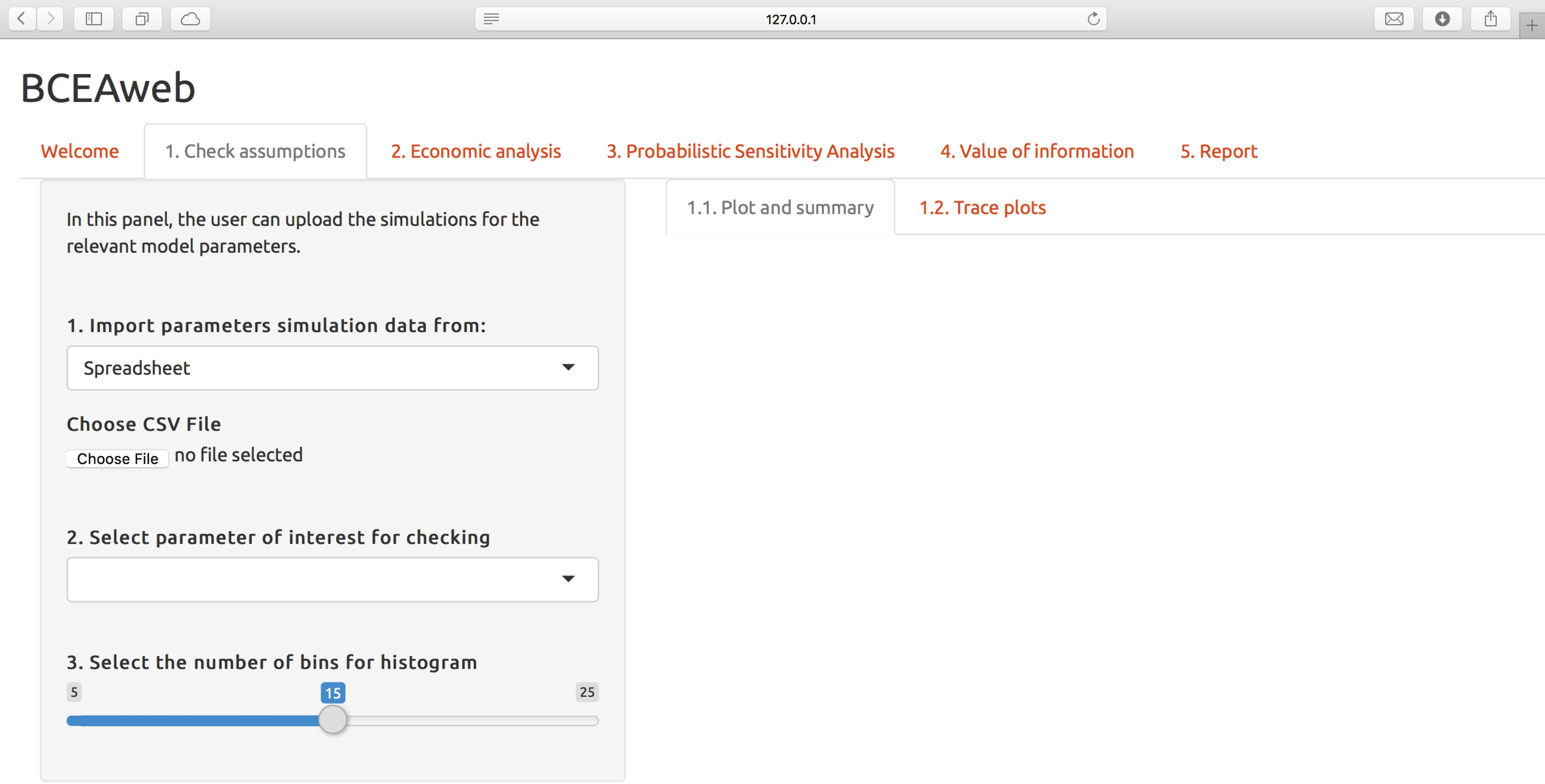
Check assumptions tab before importing any data. The left section is reserved for inputs and parameters, while outputs are displayed on the right side of the page.
The drop-down menu at the top of the grey box on the left of the page allows for selecting the preferred input data format. The data can be fed into the web app in three different formats:
- Spreadsheet, by saving the simulations in a
csv(comma-separated values) file. This is particularly useful if the simulations are produced in a spreadsheet program, such asMS Excel,LibreOfficeorGoogle Sheets; BUGS, if the values of the parameters were obtained in a software such asOpenBUGSorJAGS. The user will be required to upload the index file and a number ofCODAfiles equal to the number of simulated Markov chains;R, by providing anRDSfile obtained by saving an object (using thesaveRDSfunction) obtained from aBUGSprogram inRcontaining the values of the simulations, or alternatively passingRobjects to theBCEAweb()function if launched locally.
For online use, the data need to be saved on a file (or files, in the case of a CODA input from a BUGS program) which will be imported into BCEAweb. The content of the files need to be formatted in a standardised way so that the web app can successfully import it. The data formats for the files are described below.
5.2.6.1 Importing parameter simulation data files in BCEAweb
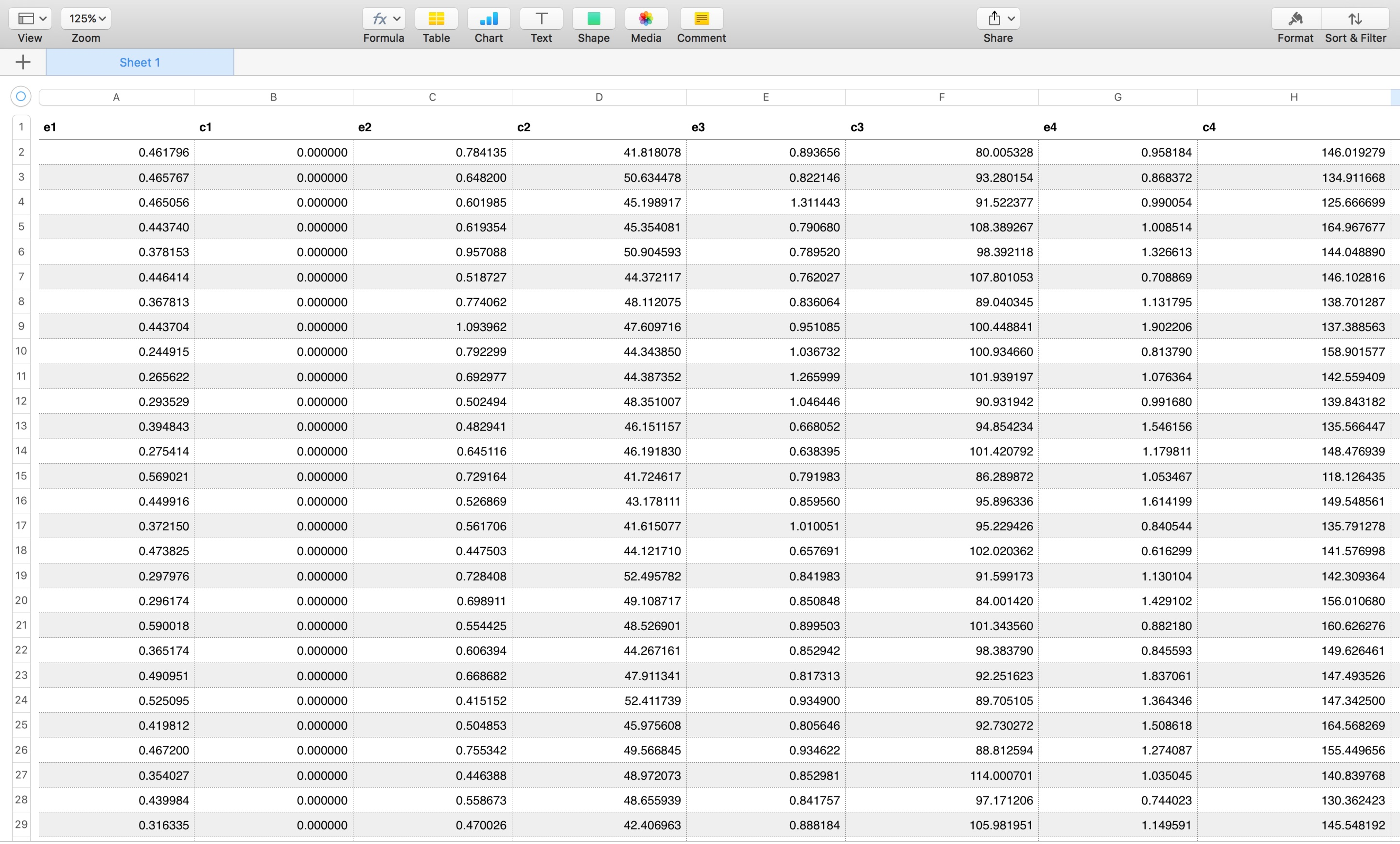
The spreadsheet input form is the easiest way to provide inputs if the economic model is programmed in a software such as MS Excel, as the parameters can be easily exported in a csv file. The data need to be arranged in a matrix with parameters by column and iterations by row, as shown in Figure 5.3. The first row is reserved for the parameter names.

csv files to be imported in the Check assumptions tab of BCEAweb. The first row is dedicated to the names of the parameters, which will be used by the web app to populate the parameter menus.
To import the values of simulations performed in R using a BUGS program such as OpenBUGS or JAGS, it is necessary to save the output object into an RDS file. The output object (\(e.g.\) obtained from the jags function) needs to be of list mode, with the list of simulations values located in the subset $BUGSoutput$sims.matrix. This is the default behaviour of the BUGS to R connection packages. The object needs to be saved (with any name) in an external file by using the saveRDS function.
If the simulations are performed directly in a BUGS program, the easiest way to import the results into BCEAweb is to save the sampled values as CODA files. Any number of chains can be imported in the web app. A file for each of the chains in addition to the CODA index file will have to be produced and uploaded into BCEAweb.
Importing a file using either the R or BUGS format will make additional functionalities available. These are diagnostic tools useful for checking for convergence and presence of autocorrelation in the series, as described in Section 5.2.6.2 below.
5.2.6.2 Using the Check Assumptions tab
The page will display a loading bar showing the transfer status of the data. As soon as the input files are imported, the web app will immediately show an histogram of the distribution of the first parameter in the dataset, together with a table reporting summary statistics of the parameter distribution at the bottom of the chart, as depicted in Figure 5.4. The variables to be displayed can be picked from the menu on the left side of the page, either by clicking on the menu and selecting one in the list or by typing the parameter label in the box, which will activate the search function. The width of the histogram bars can also be set by varying the number of bins using the slider at the bottom of the left side of the page. A greater number of bins will increase the number of bars (\(i.e.\) decreasing the number of observations per rectangle), while decreasing the number of bins will increase their size, reducing the number of bars.
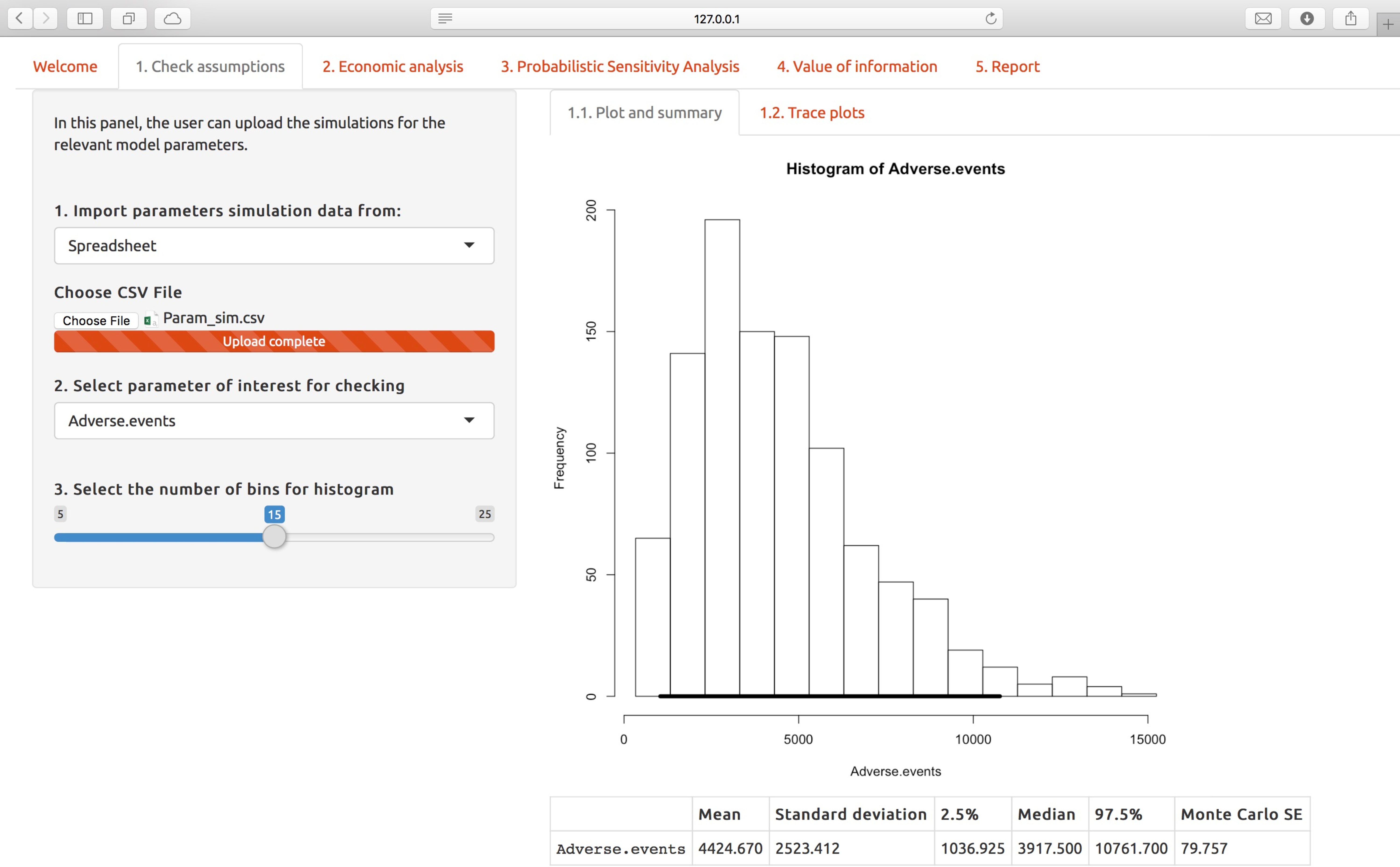
Check assumptions tab after data have been imported in a spreadsheet form. Additional analysis tools are available when importing simulations in the R or BUGS format (not shown here).
Trace plots can be shown for each parameter distribution by clicking on the respective button in the navigation bar. This functionality is not very useful when importing data from a spreadsheet as it can only show whether there are any unexpected sampling behaviours dependent on the iteration number. On the other hand if the simulations are passed to BCEAweb in a BUGS or R format and the values are sampled from multiple, parallel chains, these can be easily compared variable by variable using the trace plots.
Additional tools are available if the input data are from multiple parallel chains and imported in the web app in the BUGS or R format. By choosing one of these two options in the input format menu bar, additional navigation buttons will appear compared to the spreadsheet input option. By clicking on them, additional diagnostic tools will appear, useful for checking the convergence of Markov chains and the presence of correlation: the Gelman-Rubin plots and an analysis of the effective sample size and of the autocorrelation. These are not included when importing data from a spreadsheet as generally electronic models programmed in MS Excel or similar programs do not make use of parallel sampling from multiple chains. These tools are not discussed in detail here; interested readers can find a description of these and other diagnostics in (Baio, 2012).
5.2.7 Economic analysis
The basic analysis of the cost-effectiveness results is carried out in the “Economic analysis”. This page is the place where the cost-effectiveness results are uploaded and the starting point of the economic analysis. Analogously to the “Check assumptions” tab, the user can upload the results of a probabilistic model in three different formats: spreadsheet, BUGS and R. The data need to be arranged as already explained in the previous Section for each of the available formats, with parameters by columns and iterations by row. The parameters need to be ordered so that the health outcomes and costs for each intervention are alternated, as shown in Figure 5.5.
Economic analysis” tab. The first row is reserved for variable names which are not used but included for consistency with the input format of the “Check assumptions” tab.
The same data arrangement is required if supplying the values in the R format: health outcomes and costs need to be provided, alternated for each of the included comparisons, in a matrix or data.frame object. This object needs to be saved in RDS format using the saveRDS function for the web app to be able to read it. Health outcomes and costs must be provided in the same alternated arrangement also if using a BUGS program; one file containing the values for each of the simulated Markov chains and the CODA index file need to be uploaded onto the web app.
The “Economic analysis” page, displayed in Figure 5.6, allows choosing the parameters to be used by the underlying BCEA engine to analyse the results. On the left side of the page the user can define the grid of willingness-to-pay (WTP) thresholds used in the analysis by specifying the threshold range and the value of the “step”, \(i.e.\) the increment from one grid value to the next. The three parameters are required to have values such that the difference between the maximum and minimum threshold is divisible by the step. The default values of BCEA produce a 501-element grid, which is generally fine enough to capture differences in the economic results conditional on the WTP. Increasing the grid density by decreasing the step value has detrimental effects on computational speed, therefore the users are advised to change the grid density carefully. The cost-effectiveness threshold can also be set in this page. This value is used as the cut-off value for the decision analysis, and is used to determine if interventions are cost-effective by comparing the chosen threshold and the ICER estimated in the economic analysis. This parameter is used in the functions included in BCEAweb, such as the cost-effectiveness plane and the cost-effectiveness summary.
Once the PSA data are uploaded to BCEAweb, additional parameters become available on the left of the page. These are the names of the compared interventions, which can be changed by the user, and the intervention chosen as reference. These parameters match the ones used in the BCEA function presented in Section 3.2. When the data are uploaded and the parameters set, the analysis is performed by clicking on the “Run the analysis” grey button at the bottom of the page. The page will display the cost-effectiveness summary, as shown in Figure 5.6.
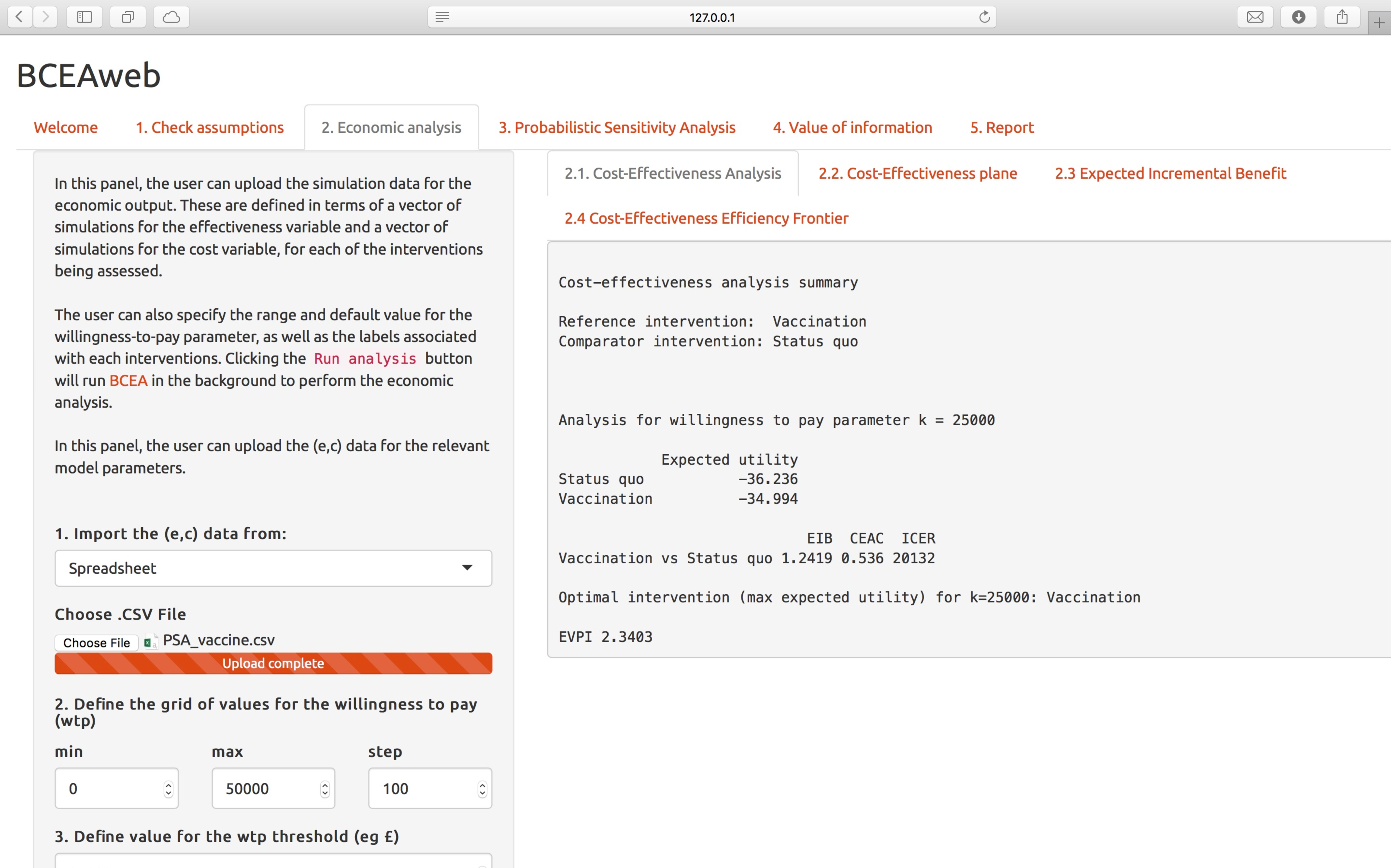
Economic Analysis” tab once the data have been uploaded and the model run. The vaccine example was used to produce the results in the Figure.
As soon as the analysis is run, BCEAweb produces the cost-effectiveness analysis summary, the cost-effectiveness plane, the expected incremental benefit plot and the cost-effectiveness efficiency frontier. These can be accessed by clicking in the sub-navigation bar; each of them will display the respective standardise output produced by BCEA:
- “
2.1 Cost-effectiveness analysis” shows the analysis summary (Section 3.3), also included in Figure 5.6; - “
2.2 Cost-effectiveness plane” includes the cost-effectiveness plane (Section 3.4). The appearance of the graph can be changed by selecting a different reference intervention and by varying the value of the WTP threshold, which will interactively (\(i.e.\) without the need of re-running the analysis) change the cost-effectiveness acceptability region; - “
2.3 Expected incremental benefit” shows the EIB plot (presented in Section 3.5), including the 95% credible intervals and the break-even point(s), if any; - “
2.4 Cost-effectiveness efficiency frontier”, which includes the efficiency frontier plot and summary table. The efficiency frontier plot is described in Section 3.7.
5.2.8 Probabilistic sensitivity analysis
The probabilistic sensitivity analysis (PSA) tab of BCEAweb includes tools to determine the uncertainty associated to the decision-making process. This section of the web app is focused on calculating and summarising the probability of cost-effectiveness of the compared interventions. The calculations in this tab are based on the data uploaded to the web app in the “Economic analysis” tab. If the importing procedure has already been carried out, the results are available to all tabs of the web app, and there is no need do re-upload them. In this case the “Probabilistic sensitivity analysis” page does not require any other input, and the graphs will be automatically displayed.
The “Probabilistic sensitivity analysis” is structured in three sub-sections. Each of them contains a different tool to analyse the probability of cost-effectiveness of the compared interventions: the pairwise cost-effectiveness acceptability curve (CEAC), the multiple-comparison CEAC and the cost-effectiveness acceptability frontier (CEAF). These tools are described in more detail in Section 4.2.2.
The plots are shown automatically if the data have already been imported into the web app (if not, these will have to be re-uploaded from the “Economic analysis” tab). The page will appear as shown in Figure 5.7. The three curves can be accessed by clicking on the respective buttons in the navigation sub-menu on the top-left corner of the page. The pairwise CEAC and the CEAF values can be downloaded by clicking on the “Download CEAC table” (or “Download CEAF table” for the frontier). This will let the user download a file in format csv including the values of the CEAC (or CEAF). Additionally the CEAC or CEAF estimates can be queried for any given threshold value included in the grid approximation (specified in the “Economic analysis” tab) directly in the web app. Changing the wtp value in the drop-down menu will return the respective probability of cost-effectiveness. However if multiple interventions are compared, as in Figure 5.7, the CEAC value shown will refer to the first curve plotted. In the case shown the CEAC values shown (\(i.e.\) 0.6600) indicates the probability of “Group counselling” being cost-effective when compared to “No contact”.
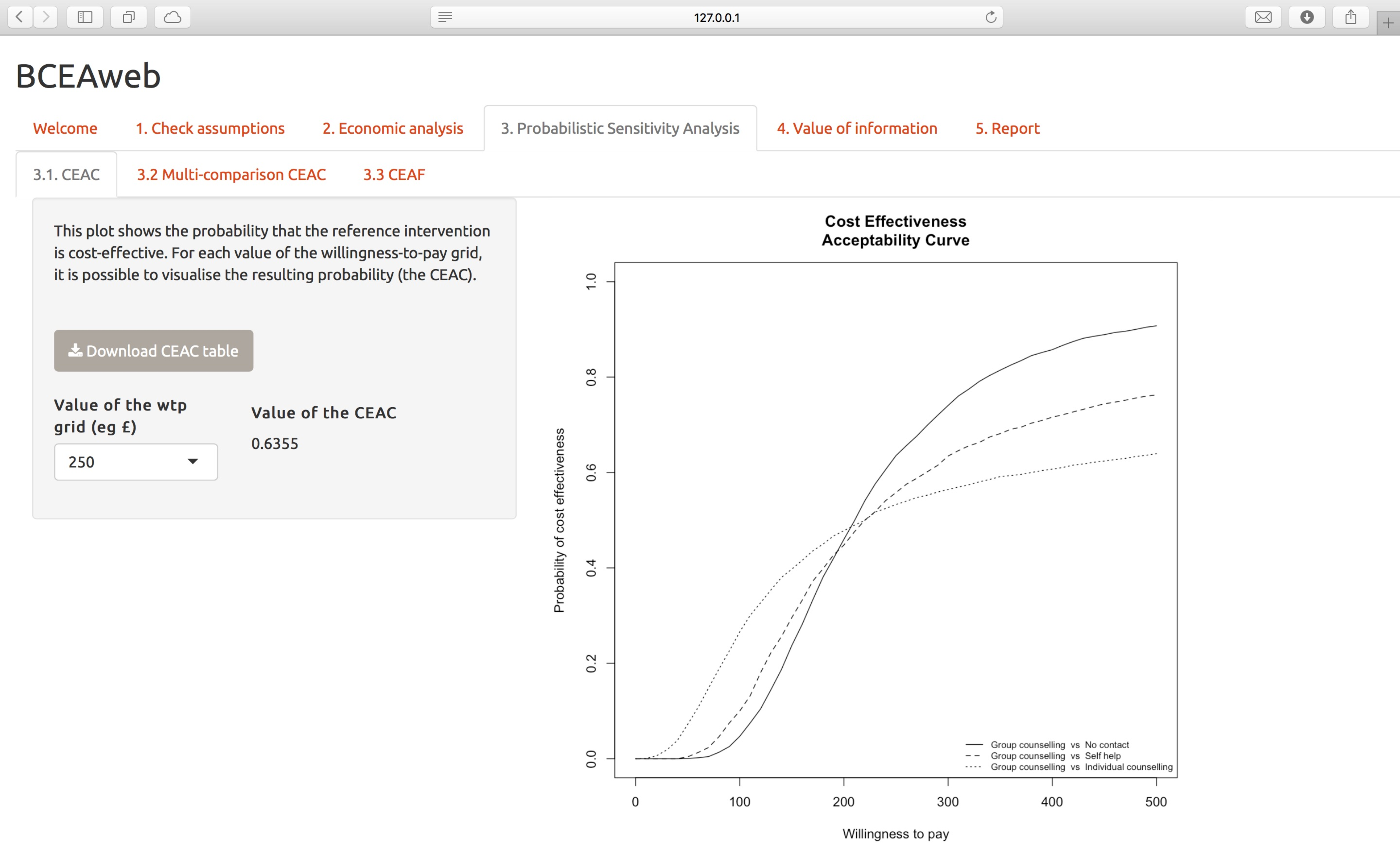
Probabilistic sensitivity analysis” tab, showing the cost-effectiveness acceptability curves for the smoking cessation example.
5.2.9 Value of information
The “Value of information” tab is focused on three tools for the value of information analysis:
- Expected value of perfect information, or EVPI, is the monetary value (based on the monetary net benefit utility function) attributable to reducing the overall uncertainty in the economic model (and thus in the decisional process);
- Expected value of partial perfect information, or EVPPI, is the value attributable to a reduction in the uncertainty associated to a single parameter or to a specific set of parameters in the economic model;
- Info-rank plot, an extension of the tornado plot, is useful to assess how parameters contribute to the uncertainty in the model by ordering them in decreasing order of the ratio of single-parameter EVPPI on EVPI in correspondence of a given WTP threshold (shown in Figure 5.8).
The EVPI tab works in a similar fashion to the CEAC one, as it does not require any other data than the PSA data imported into the web app form the “Economic analysis” tab. Analogously to the CEAC, the values can be explored by using the drop-down menu in the page, as well as downloaded in a csv file by clicking on the “Download EVPI table” button.
The “Info-rank” and “EVPPI” require that both the parameter simulations, uploaded in the “Check assumptions” tab, and the probabilistic economic results, uploaded in the “Economic analysis” tab, are available. If these are not fed into BCEAweb, it will not possible to calculate the EVPPI and the info-rank table. Once both parameter values and economic results are correctly imported, the parameter selection menus in the “Info-rank” and “EVPPI” tabs (labelled “Select relevant parameters” and “Select parameters to compute the EVPPI”, respectively) will display a list of the model parameters. These can be either selected from the drop-down menu or searched by typing the parameter labels into the menu field. Any number of parameters can be selected; choosing “All parameters” selects all of them at the same time. The analyses are run by selecting the parameters and clicking on the grey “Run” button at the bottom of the page. In addition the EVPI, EVPPI and Info-rank tables of values can be downloaded in csv format by clicking on the grey “Download” button.
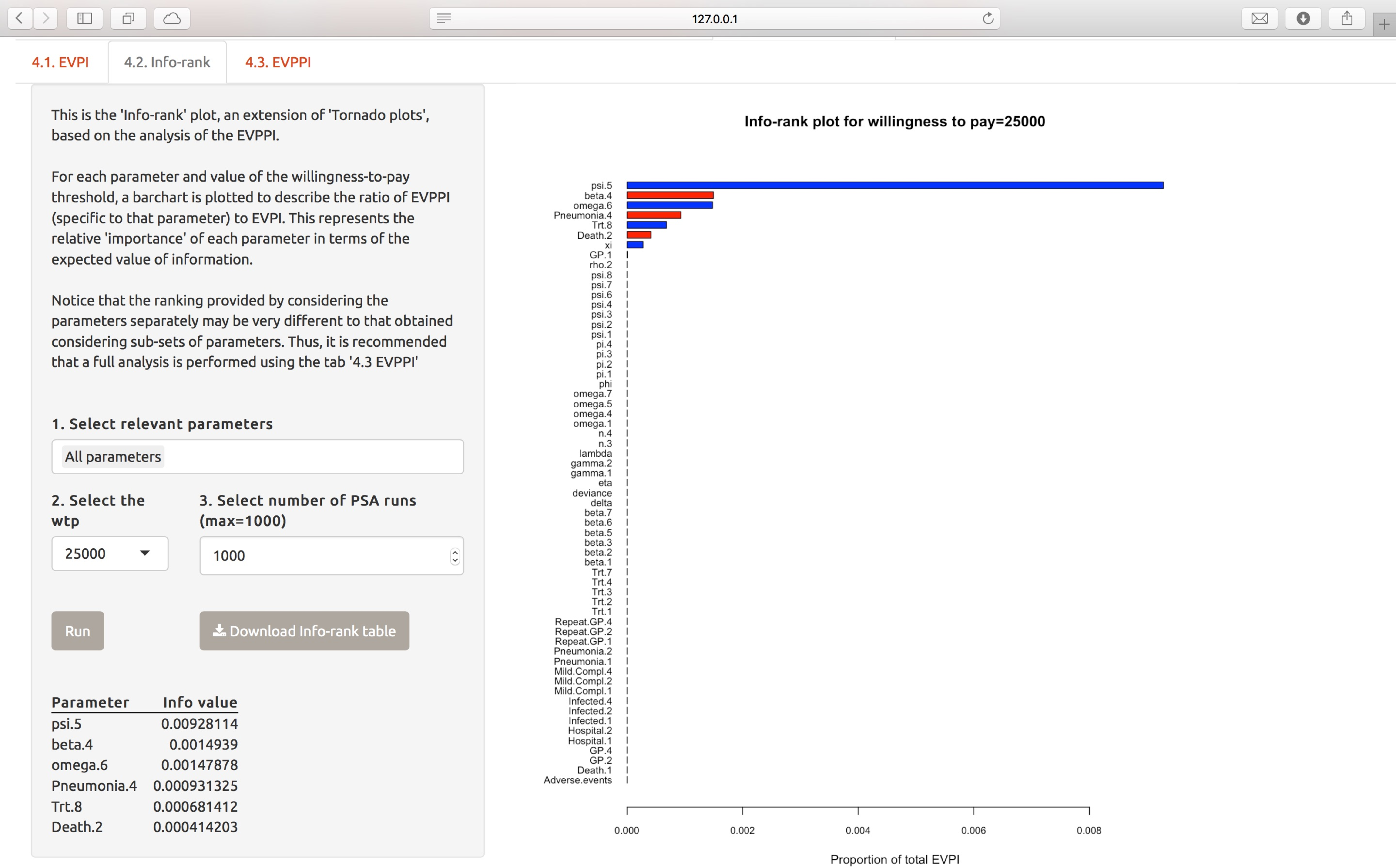
Info-rank plot for the vaccine example, including all parameters, in correspondence of a threshold of 25,000 monetary units. While the psi.5 parameter stands out compared to the other variables, the proportion between the single-parameter EVPPI and total EVPI is below 1%.
The EVPPI tab in BCEAweb includes alternative methods for the estimation of the EVPPI, and allows for fine-tuning the parameters of the procedure based on the chosen methodology. In addition to a plot comparing the full-model EVPI and the EVPPI for the selected parameter (or set of parameters), BCEAweb also includes a “Diagnostic” tab, which can be accessed from the EVPPI page. It includes residual plots for both the costs and outcomes, so that the user can check for unexpected behaviours in the model fit which might make the EVPPI estimates unreliable. BCEAweb allows for easy checking of the reliability of the estimation and also gives the instruments to intervene on simple issues; for example non-linearities in the distribution of the residuals can be addressed by increasing the interaction order using the INLA-SPDE estimation method.
5.2.10 Report
The “Report” tab allows downloading the outputs produced by BCEAweb in a standardised report, which can be downloaded in a pdf or Microsoft Word format. The list of sections is displayed on the page, and checking the respective box will include the output section in the report produced by the web app. It is worth noting that the correct data need to be available for each section to be produced correctly. The outputs produced in the report will depend on the parameters specified in the BCEAweb tabs for each of the selected sections, \(e.g.\) the comparator names, the variables included in the EVPPI analysis, etc.
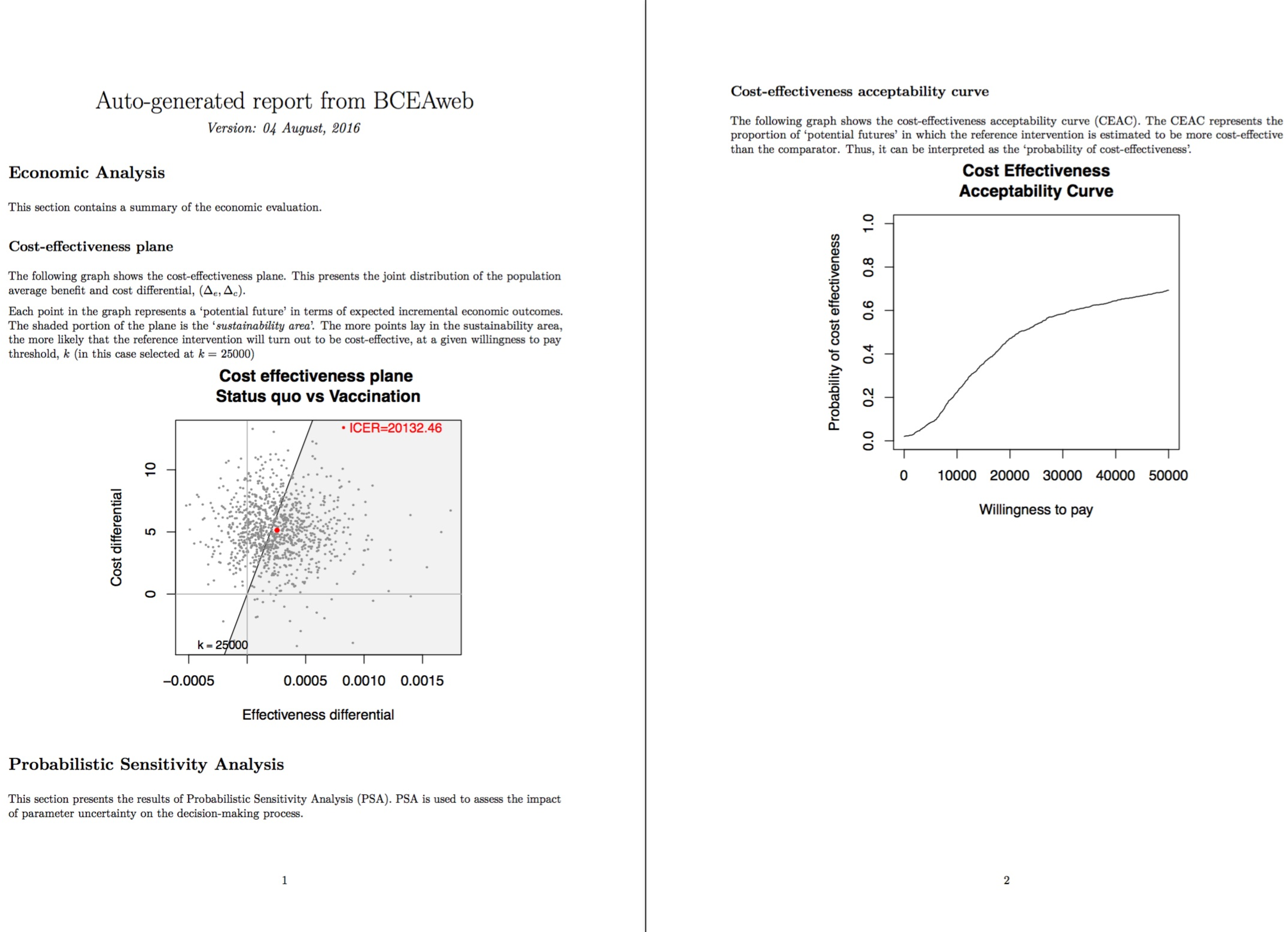
BCEAweb for the vaccine example. This report was obtained by selecting the cost-effectiveness plane and CEAC sections only.
To download the report from BCEAweb it is sufficient to select the section required by the user, choose the preferred output format and click on the grey “Download” button at the bottom of the page. The report will be generated and downloaded; please note that in some internet browsers, depending on the user settings, the report might be displayed as a new web page. An example of a report generated by the web app for the vaccine example is shown in Figure 5.9. The cost-effectiveness plane and cost-effectiveness acceptability curve sections were selected to produce the report for the vaccine example.
References
Baio, G., 2012. Bayesian Methods in Health Economics. Chapman Hall/CRC Press, Boca Raton, FL.
Chang, W., Cheng, J., Allaire, J., Xie, Y., McPherson, J., 2015. Shiny: Web application framework for r.
Hart, R., Burns, D., Strong, M., Berardi, A., Lee, D., 2025. R and Shiny in HTA, in: Baio, G., Thom, H., Pechivanoglou, P. (Eds.), R for Health Technology Assessment.
Heath, A., Manolopoulou, I., Baio, G., 2016. Estimating the expected value of partial perfect information in health economic evaluations using integrated nested Laplace approximation. Statistics in Medicine. https://doi.org/10.1002/sim.6983
Strong, M., Oakley, J., Brennan, A., 2014. Estimating Multiparameter Partial Expected Value of Perfect Information from a Probabilistic Sensitivity Analysis Sample A Nonparametric Regression Approach. Medical Decision Making 34, 311–326.