4 Probabilistic sensitivity analysis using BCEA
4.1 Introduction
Theoretically, as mentioned in Section 1.3, the maximisation of the expected utility is all that is required to determine the best course of action in the face of uncertainty and given current evidence (Baio, 2012; Baio and Dawid, 2011; Claxton, 1999). This means that if we completely trust all the assumptions made in the current modelling and the data used to inform the unobserved and unobservable quantities, then the computation of ICERs and EIBs would be sufficient to determine which treatment is the most cost-effective. The decision-making process would therefore be completely automated under these circumstances. This implies that, as shown throughout Chapter 3, the vaccination strategy and the Group Counselling interventions would be implemented immediately for willingness to pay values of 25,000 and 250 monetary units respectively in the two examples of Chapter 2.
Of course, in reality this is hardly ever a realistic situation: the evidence upon which the statistical model is based is often limited (either in size, or time follow-up, or in terms of generalisability to a reference population). In addition, any statistical model represents an idealisation of a complex reality and inevitably fails to account for all the relevant aspects that may determine future outcomes. Therefore, while theoretically the ICER or alternatively the EIBs contains all the relevant information for decision making, it is often important to consider the uncertainty associated with the underlying process.
This is particularly true in economic evaluations, where the objective of the analysis is not simply inference about unknown quantities, but to drive policy decisions which involve investing significant resources on the “optimal” intervention. More importantly, investment in one intervention involves removing investment from other alternatives. Additionally, some interventions may require significant upfront investment that would be wasted if, in the light of new evidence, the intervention was non-optimal. Therefore, in general, decision makers must understand the uncertainty surrounding their decision. If this uncertainty is high they will, typically, recommend future research is carried out before resources are invested in new treatments. For this reason, health technology assessment agencies such as NICE in the UK recommend the application of Probabilistic Sensitivity Analysis (PSA) to the results of an economic evaluation.
This chapter will introduce PSA, which is used to test the impact of the model uncertainty and model assumptions in the optimal decision, as well as several techniques that are used to summarise, quantify and analyse how uncertainty influences the decision-making process. This analysis can be divided into two parts, depending on the source of the uncertainty. The first two sections of this chapter will focus on parameter uncertainty. This explores the impact of the uncertainty associated with the model parameters on the decision-making process. In a Bayesian setting this parametric uncertainty is captured by the posterior distributions for the parameters and can be thought of as the uncertainty present conditional on the assumptions of the health economic model. Both the examples introduced in Chapter 3 are used to illustrate the different tools available in BCEA, built to understand and report the impact of the parametric uncertainty.
The final section of this chapter (Section 4.4) will then introduce the concept of PSA applied to structural uncertainty. This is concerned with analysing the influence of the model assumptions themselves. Clearly, this type of analysis has a very broad scope but within BCEA we focus on two key elements of structural uncertainty. These are the impact of the implicit assumptions coming from the health economic modelling framework, such as risk aversion, and the impact of alternative model specifications, such as changing the prior distribution for certain parameters. The capabilities of BCEA for structural PSA is illustrated, again, with practical~examples.
4.2 Probabilistic sensitivity analysis for parameter uncertainty
In a nutshell, PSA for parameter uncertainty is a procedure in which the input parameters are considered as random quantities. This randomness is associated with a probability distribution that describes the state of the science [i.e. the background knowledge of the decision-maker; Baio (2012)]. As such, PSA is fundamentally a Bayesian exercise where the individual variability in the population is marginalised out but the impact of parameter uncertainty on the decision is considered explicitly. Calculating the ICER and EIB averages over both these sources of uncertainty as the expected value for the utility function is found with respect to the joint distribution of parameters and data. This parametric uncertainty is propagated through the economic model to produce a distribution of decisions where randomness is induced by parameter uncertainty.
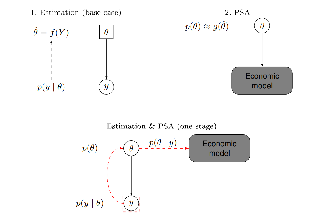
From the frequentist point of view, PSA is unintuitive as parameters are not considered as random quantities and therefore are not subject to epistemic uncertainty. Consequently, PSA is performed using a two-stage approach. Firstly, the statistical model is used to estimate the parameters, \(e.g.\) using the Maximum Likelihood Estimates (MLEs) \(\hat\theta\) as a function of the observed data, say \(y\). These estimates are then used to define a probability distribution describing the uncertainty in the parameters, based on a function \(g(\hat\theta)\). For example, the method of moments could be used to determine a suitable form for a given parametric family (\(e.g.\) Normal, Gamma, Binomial, Beta, etc.) to match the observed mean and, perhaps, standard deviation or quantiles. Random samples from these “distributions” are obtained (\(e.g.\) using random number generators, which for simple distributions are available even in spreadsheet calculators such as MS Excel) and finally fed through the economic model (see Figure 1.5) to find a distribution for the decisions, much as in the same way as in the Bayesian setting.
Figure 4.1 illustrates the fundamental difference between the two approaches. The top panel shows the frequentist, two-stage process, while the bottom panel depicts the one-step Bayesian analysis. In the former, the parameter \(\theta\) is a fixed quantity (represented in a square, in the top-left panel). Sampling variability is modelled as a function of the parameter \(p(y\mid \theta)\); this is used to obtain the estimate of the “true” value of the parameter, \(\hat\theta\). In a separate step (the top-right panel), the analysis “pretends” that the parameters are actually random (and hence depicted in a circle, in the top-right panel) and associated with a probability distribution defined in terms of \(\hat\theta\) (or a function thereof). In the Bayesian analysis in the bottom panel, the parameter is considered as a random variable in the first place (and hence it is depicted in a circle in the bottom panel); as soon as data \(y\) become available, the uncertainty on \(\theta\) is updated and automatically propagated to the economic model.
The most relevant implication of the distinction between the two approaches is that a frequentist analysis typically discards the potential correlation among the many parameters that characterise the health economic model. This is because the uncertainty in \(\theta\) is typically defined by a set of univariate distributions \(p(\theta_q)\), for each of the \(q=1,\ldots,Q\) model parameters. We do note, however, that while it is possible to use a multivariate distribution to account for correlation between the parameters, most models developed under a frequentist approach (for which computations are often performed in Excel) are not based on these more complex distributions.
Conversely, a full Bayesian model can account for this correlation automatically as the full joint posterior distribution \(p(\pmb\theta) = p(\theta_1,\ldots,\theta_Q)\) is typically generated, usually using MCMC, and propagated to the economic model. Interestingly, even if some form of independence is assumed in the prior distributions, the model structure and the observed data may induce some correlation in the posterior with no extra modelling complications as this correlation is automatically picked up in the computation of the posterior distributions.
This may help demystify the myth that “Bayesian models are more complex”: when comparing a simple, possibly univariate, frequentist model with its basic Bayesian counterpart (\(e.g.\) based on “minimally informative” priors), it is perhaps fair to say that the latter involves more complicated computation. However, when the model is complex to start with (\(e.g.\) based on a large number of variables, or characterised by highly correlated structures), then the perceived simplicity of the frequentist approach is rather just a myth and, in fact, a Bayesian approach usually turns out as more effective, even on a computational level.
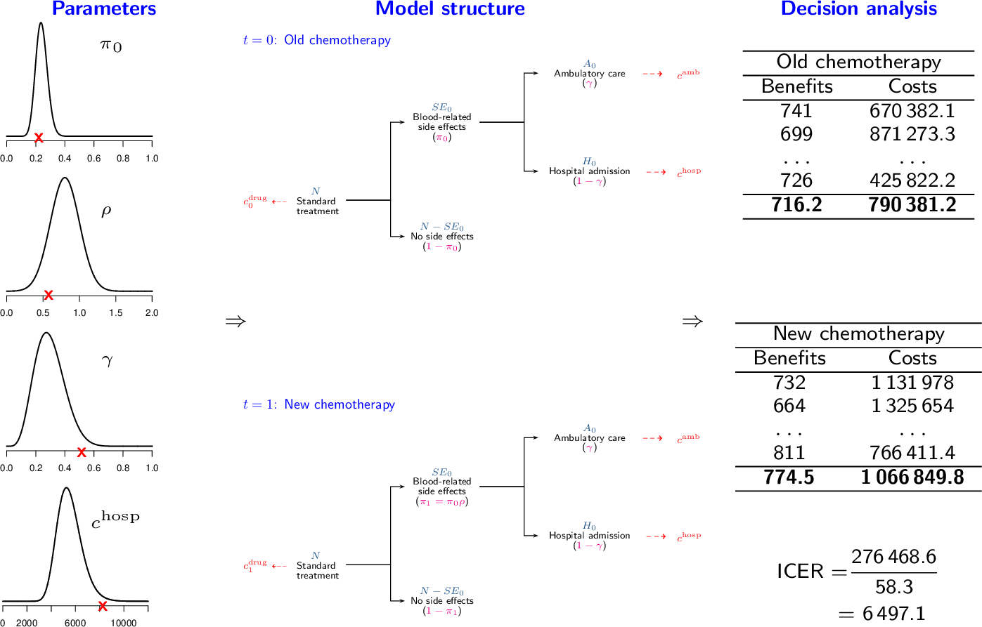
Figure 4.2 gives a visual indication of the PSA process where the parameter distributions seen on the left-hand side of the figure can be determined in a Bayesian or frequentist setting. PSA begins by simulating a set of parameter values, represented by red crosses in Figure 4.2). These parameter values are then fed through the economic model to give a value for the population summaries \((\Delta_e,\Delta_c)\), shown in the middle column in Figure 4.2 and recorded in the final column “Decision Analysis”. These measures are then combined to perform the cost-effectiveness analysis and calculate a suitable summary, \(e.g.\) IB\((\pmb\theta)\), for the specific simulation. This process is replicated for another set of the simulated values to create a table of \((\Delta_e,\Delta_c)\) for different simulations, along with a table of summary measures. Note that if the functions used to compute \((\Delta_e,\Delta_c)\) are non-linear, PSA does not simply allow you to assess the impact of parameter uncertainty on the decision but is, in fact, required to accurately compute the ICER or EIB. This is because the expected value of a non-linear function is not equal to the function evaluated at the expected value of the model parameters.
As PSA provides a a table of \((\Delta_e,\Delta_c)\) for each simulation, PSA is integral to the analysis framework used in BCEA which is based on a simulation approach from the distribution of \((\Delta_e, \Delta_c)\). Doing the full economic analysis involves summarising this table using a suitable summary such as the ICER. However, PSA involves considering the distribution of the final summary measure such as the row-wise IB\((\pmb\theta)\). This gives a decision for each row of the PSA table, conditional on the parameter values in that specific simulation. This actually implies that one the main tools to evaluate the parameter uncertainty is the cost-effectiveness plane, because it provides helpful information about how the model output varies due to uncertainty in the parameters. However, to further extend the analysis of this decision uncertainty, the impact of parameter uncertainty on the decision-making process can be assessed for different willingness to pay values.
4.2.1 Summary tables
BCEA provides several types of output that can be used to assess the health economic evaluation. As seen in Chapter 3, a summary can be produced as follows:
summary(m)where m is a bcea object. This function provides the output reported in Section 3.3.
In addition to the basic health economic measures, \(e.g.\) the EIB and the ICER, BCEA provides some summary measures for the PSA, allowing a more in-depth analysis of the variation observed in the results, specifically the CEAC Section 4.2.2 and the EVPI Section 4.3.1. The full output of the PSA is stored in the bcea object, and can be easily accessed using the function sim_table, \(e.g.\) with the following code.
table <- sim_table(m, wtp=25000)The willingness to pay value (indicated by the argument wtp) must be selected from the values of the grid generated when the bcea object was created, as in the summary function (see Section 3.3) and is set to \(25,000\) monetary units or Kmax when that argument has been used by default.
The output of the sim_table function is a list, composed of the following elements:
Table: the table in which the output is stored as a matrix;names.cols: the column names of theTablematrix;wtp: the chosen willingness to pay value threshold. All measures depend on it since it is a parameter in the utility function;ind.table: the index associated with the selectedwtpvalue in the grid used to run the analysis. It is the position thewtpoccupies in them$kvector, wheremis the originalbceaobject.
The matrix Table contains the health economics outputs for each simulation and can be accessed by subsetting the object created with the sim_table function. The first lines of the table can be printed in the R console as follows:
head(table$Table) U1 U2 U* IB2_1 OL VI
1 -36.57582 -38.71760 -36.57582 -2.1417866 2.141787 -1.750121
2 -27.92514 -27.67448 -27.67448 0.2506573 0.000000 7.151217
3 -28.03024 -33.37394 -28.03024 -5.3436963 5.343696 6.795451
4 -53.28408 -47.13734 -47.13734 6.1467384 0.000000 -12.311646
5 -43.58389 -40.40469 -40.40469 3.1791976 0.000000 -5.578996
6 -42.37456 -33.08547 -33.08547 9.2890987 0.000000 1.740230Note that this particular excerpt presents the results from the Vaccine example. The table is easily readable and reports for every simulation, indexed by the leftmost column, the following quantities:
U1andU2: the utility values for the first and second intervention. When multiple comparators are included, additional columns will be produced, one for every considered comparator;U*: the maximum utility value among the comparators, indicating which intervention produced the most benefits at each simulation;IB2_1: the incremental benefit IB for the comparison between intervention 2 and intervention 1. Additional columns are included when multiple comparators are considered (\(e.g.\)IB3_1);OL: the opportunity loss, obtained as the difference between the maximum utility computed for the current parameter configuration (\(e.g.\) at the current simulation)U*and the current utility of the intervention associated with the maximum utility overall. In the current example and for the selected threshold of willingness to pay, the mean of the vectorU1, where the vaccine is not available, is lower than the mean of the vectorU2, vaccine available, as vaccination is the most cost-effective intervention, given current evidence. Thus, for each row of the simulations table, the OL is computed as the difference between the current value ofU*and the value ofU2. For this reason, in all simulations where vaccination is indeed more cost-effective (i.e. whenIB2_1is positive), then \(\mbox{OL}(\pmb\theta)=0\) as there would be no opportunity loss, if the parameter configuration were the one obtained in the current simulation;VI: the value of information, which is computed as the difference between the maximum utility computed for the current parameter configurationU*and the expected utility of the intervention which is associated with the maximum utility overall. In the Vaccine example and for the selected threshold of willingness to pay, vaccination (U2) is the most cost-effective intervention, given current evidence. Thus, for each row of the simulations table, the VI is computed as the difference between the current value ofU*and the mean of the entire vectorU2. Negative values of theVIimply that for those simulation specific parameter values both treatment options are less valuable than the current optimal decision, in this case vaccination.
BCEA includes a set of functions that can present the results of PSA in graphical form. We only consider the commonly used graphical displays for the PSA results, which we describe in the following section.
4.2.2 Cost-effectiveness acceptability curve
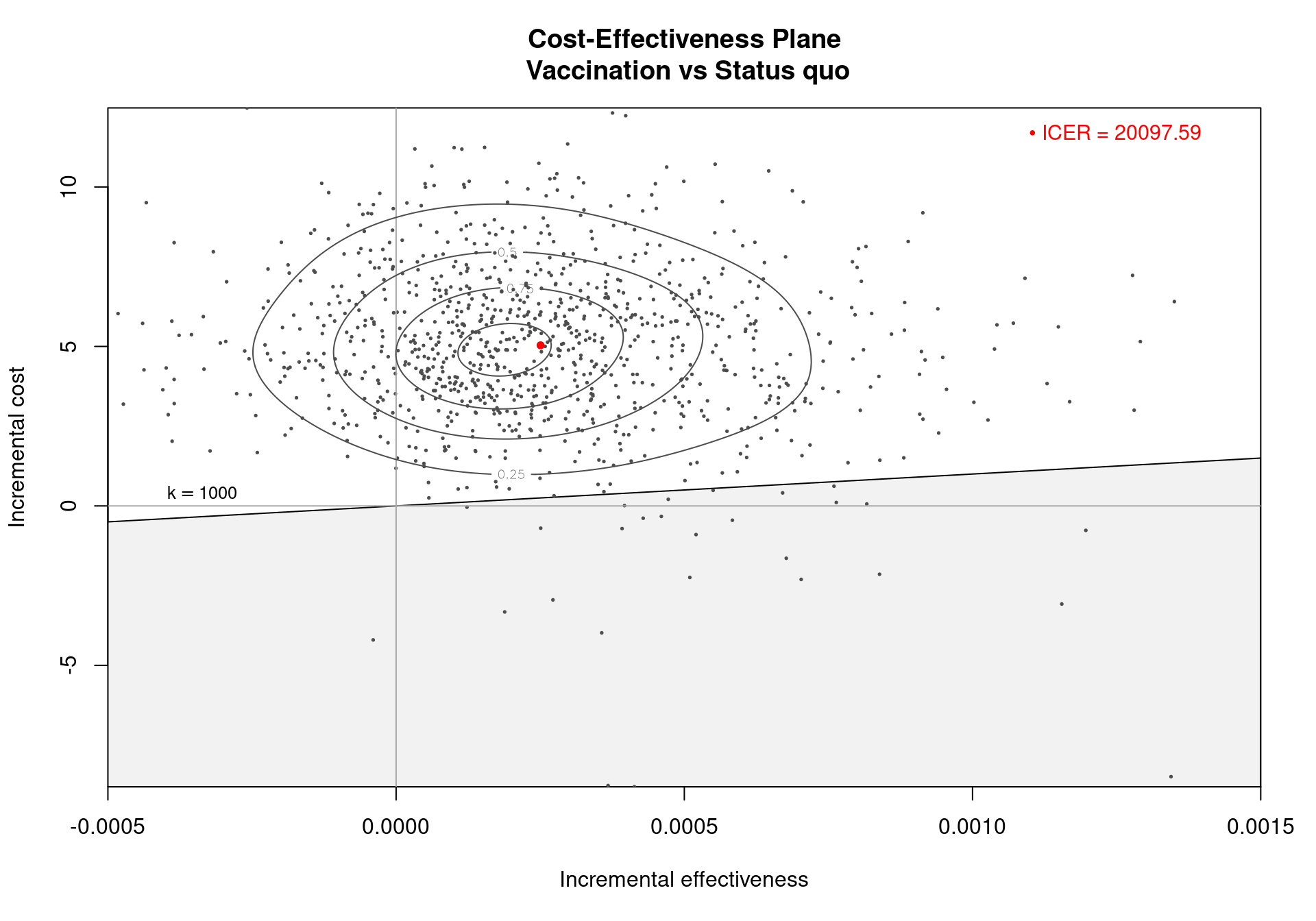
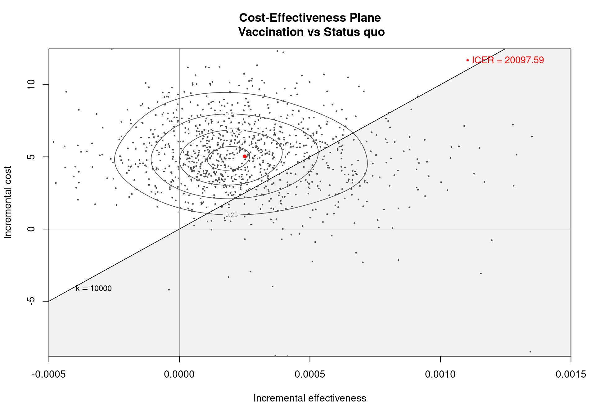
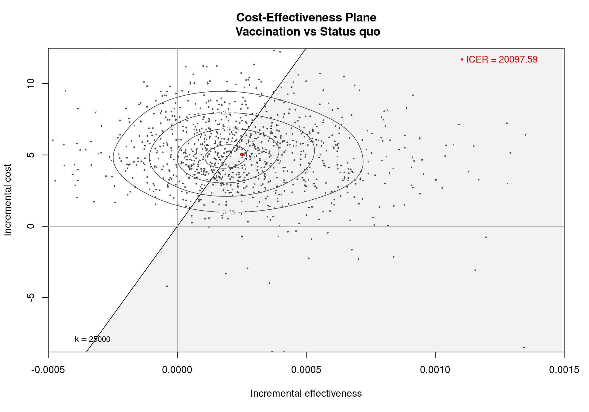
The Cost-Effectiveness Acceptability Curve (CEAC), originally proposed in (Hout et al., 1994), estimates the probability of cost-effectiveness for a given intervention, for different willingness to pay thresholds. The CEAC is used to evaluate the uncertainty associated with the decision-making process, since it quantifies the degree to which a treatment is preferred. This is typically measured by comparing the net benefit of the different intervention. In particular, for a two intervention problem, we evaluate the CEAC using the incremental benefit \(\mbox{IB}(\pmb\theta)\) by defining the CEAC as \[ \text{CEAC} = \Pr(\text{IB}(\pmb\theta) > 0). \] This effectively represents the proportion of simulations in which \(t=2\) is associated with a higher utility than \(t=1\). If the net benefit function is used, the definition can be re-written as \[ \text{CEAC} = \Pr(k\Delta_e - \Delta_c > 0), \] which depends on the willingness to pay value \(k\). This means that the CEAC can be used to determine the probability that treatment 1 is optimal changes as the willingness to pay threshold increases. In addition, this shows the clear links between the analysis of the cost-effectiveness plane and the CEAC. Figure 4.3 shows in panels (a)-(c) the cost-effectiveness plane for three different choices of the willingness to pay parameter, \(k\). In each, the CEAC is exactly the proportion of points in the sustainability area. Panel (d) shows the CEAC for a range of values of \(k\) in the interval \([0 - 50\,000]\).

In a decision problem with more than two potential interventions, e.g., the smoking cessation example in Chapter 2, the CEAC can be computed in a pairwise manner. This definition uses the same formula presented above and computes the probability that each intervention is superior to the reference group. Alternatively, the CEAC can be computed overall by calculating the probability that each intervention is associated with the largest net benefit, i.e., is the simulation-specific optimal intervention. In this second definition, the CEAC values across all the interventions will sum to 1.
Note that the intervention with the highest CEAC value is not necessarily the intervention with the largest EIB value. This means that if two alternative interventions are considered and one of them has an associated CEAC value equal to 0.51, this intervention may not be associated with a positive differential in the expected net benefit. This is because the CEAC gives additional information and the ICER or EIB are measuring different elements of the decision problem and, when the PSA distribution for interventions is skewed, these two different methods of measuring the optimal intervention may not coincide. However, if the CEAC value for an intervention is high, it is more likely that the intervention is also associated with the highest EIB, even if mathematically this is not required. It is important, therefore, the consider both the ICER or EIB and the CEAC when interpreting the results from a PSA. Alternatively, the value of information (VOI) methods that are discussed in Section 4.3 can provide a more complete picture of the parametric uncertainty and its impact on decision making.
The CEAC value in correspondence of the chosen willingness to pay threshold is included by default in the summary.bcea function output, described in Section 3.3 and Section 4.2.1. Functions are included in BCEA to produce a graphical output for both pairwise and multiple comparisons.
4.2.2.1 Example: Vaccine (continued)
For the Vaccine example, the summary table in Section 3.3) reports that the CEAC is equal to \(0.529\), for a willingness to pay threshold of 25,000 monetary units. This indicates a relatively low probability of cost-effectiveness for the vaccination policy over the status quo, as the CEAC is close \(0.5\). When only two comparators are under investigation, a CEAC value equal to \(0.5\) means that the two interventions have the same probability of cost-effectiveness. This is the maximum possible probabilistic uncertainty associated with the decision making process. Therefore, a CEAC value of \(0.529\) means that, even though the vaccination is most likely to be cost-effective, the difference with the reference comparator is modest.
An alternative way of thinking of the CEAC value is to consider all “potential futures” determined by the current uncertainty in the parameters: under this interpretation, in nearly 53% of these cases \(t=1\) will turn out to be cost-effective (and thus the “correct” decision, given the available knowledge). This also states that, for a willingness to pay of \(25\,000\) monetary units, nearly 53% of the points in the cost-effectiveness plane lie in the sustainability area.
From the decision-maker’s perspective it is very informative to consider the CEAC for different willingness to pay values, as it allows to understand the level of confidence they can have in the decision. It also demonstrates how the willingness to pay influences this level of confidence. In fact, regulatory agencies such as NICE in the UK do not use a single threshold value but rather evaluate the comparative cost-effectiveness on a set interval. As the CEAC depends strongly on the chosen threshold, it can be sensitive to small increments or decrements in the value of the willingness to pay and can vary substantially.
To plot the cost-effectiveness acceptability curve for a bcea object m the function ceac.plot is used, producing the output depicted in Figure 4.4.
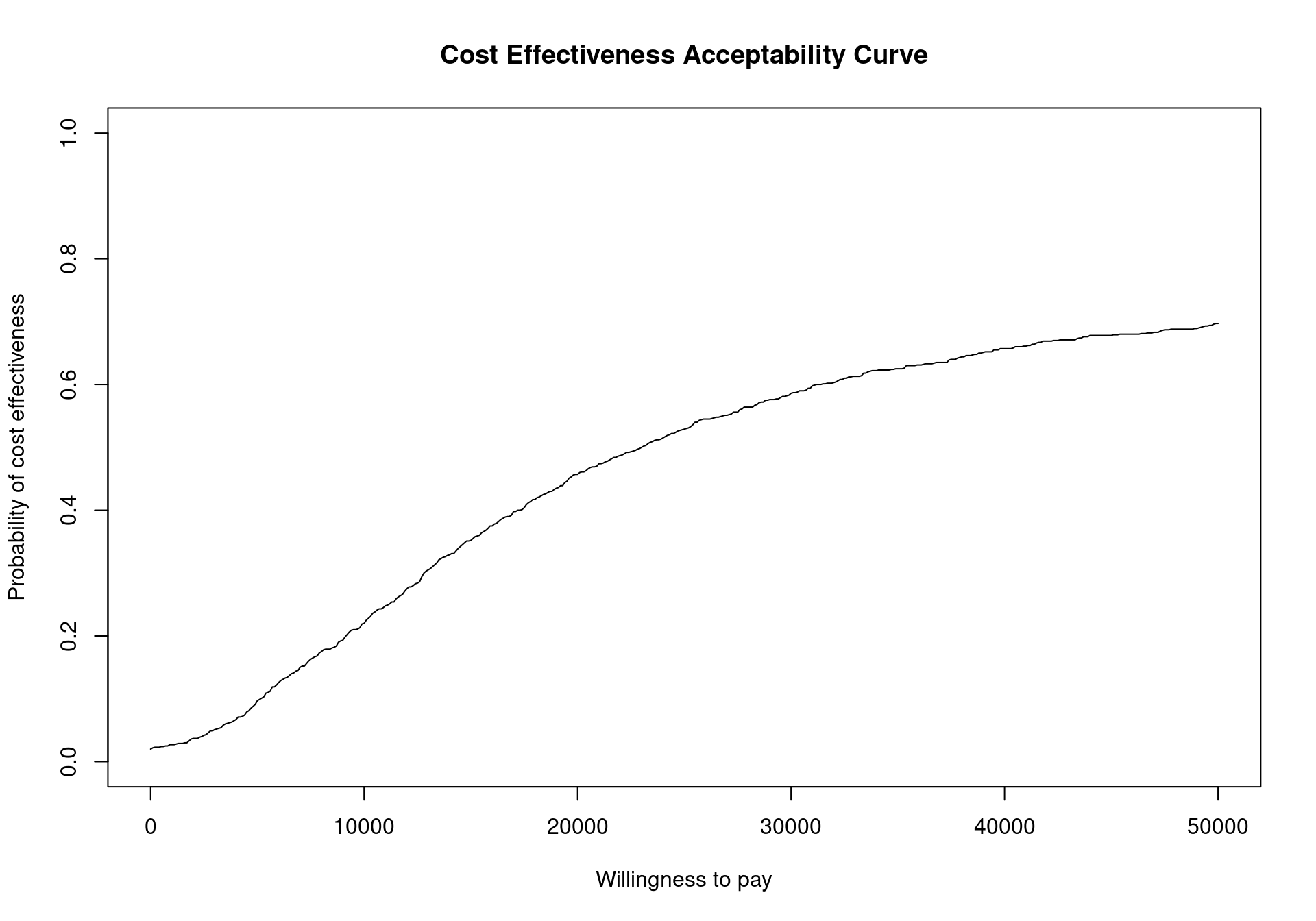
The CEAC curve in Figure 4.4 increases together with the willingness to pay. As vaccination is more expensive and more effective than the status quo, if the willingness to pay increases, a higher number of simulations yields a positive incremental benefit. In other terms, as the slope of the line defining the cost-effectiveness acceptability region on the cost-effectiveness plane increases, more points are included in the sustainability region.
The values of the CEAC for a given threshold value can be extracted directly from the bcea object by extracting the ceac element. For example the CEAC value for willingness to pay values of \(20\,000\) and \(30\,000\) monetary units will be displayed by running the following code
with(m, ceac[which(k == 20000), ])Status quo
0.457 with(m, ceac[which(k == 30000), ])Status quo
0.586 or equivalently
m$ceac[which(m$k == 20000), ]Status quo
0.457 m$ceac[which(m$k == 30000), ]Status quo
0.586 The lines above will return an error if the specified value for k is not present in the grid of willingness to pay values included in the m$k element of the bcea object m.
The CEAC plot can become more informative by adding horizontal lines at given probability values to read off the probabilities more easily (Figure 4.5). To add these lines in the base version of the plot simply call the function lines after the ceac.plot function. For example to include horizontal lines at the level \(0.25\), \(0.5\) and \(0.75\), run the following code.
ceac.plot(m)
lines(x=range(m$k), y=rep(0.5,2), col="grey50", lty=2)
lines(x=range(m$k), y=rep(0.25,2), col="grey75", lty=3)
lines(x=range(m$k), y=rep(0.75,2), col="grey75", lty=3)
R base facilities
For a single pairwise comparison, the ggplot2 version of the ceac.plot is the same as the base version, due to the simplicity of the graph. The default output is built to be consistent with the base version, meaning that it does not include a background grid. This can be easily overcome using the flexibility of the ggplot2 package. For example, it is possible to simply restore the default gridline of the theme_bw theme by executing the following lines.
ceac.plot(m, graph="ggplot") + theme(panel.grid=element_line())which create the graph displayed in Figure 4.6.
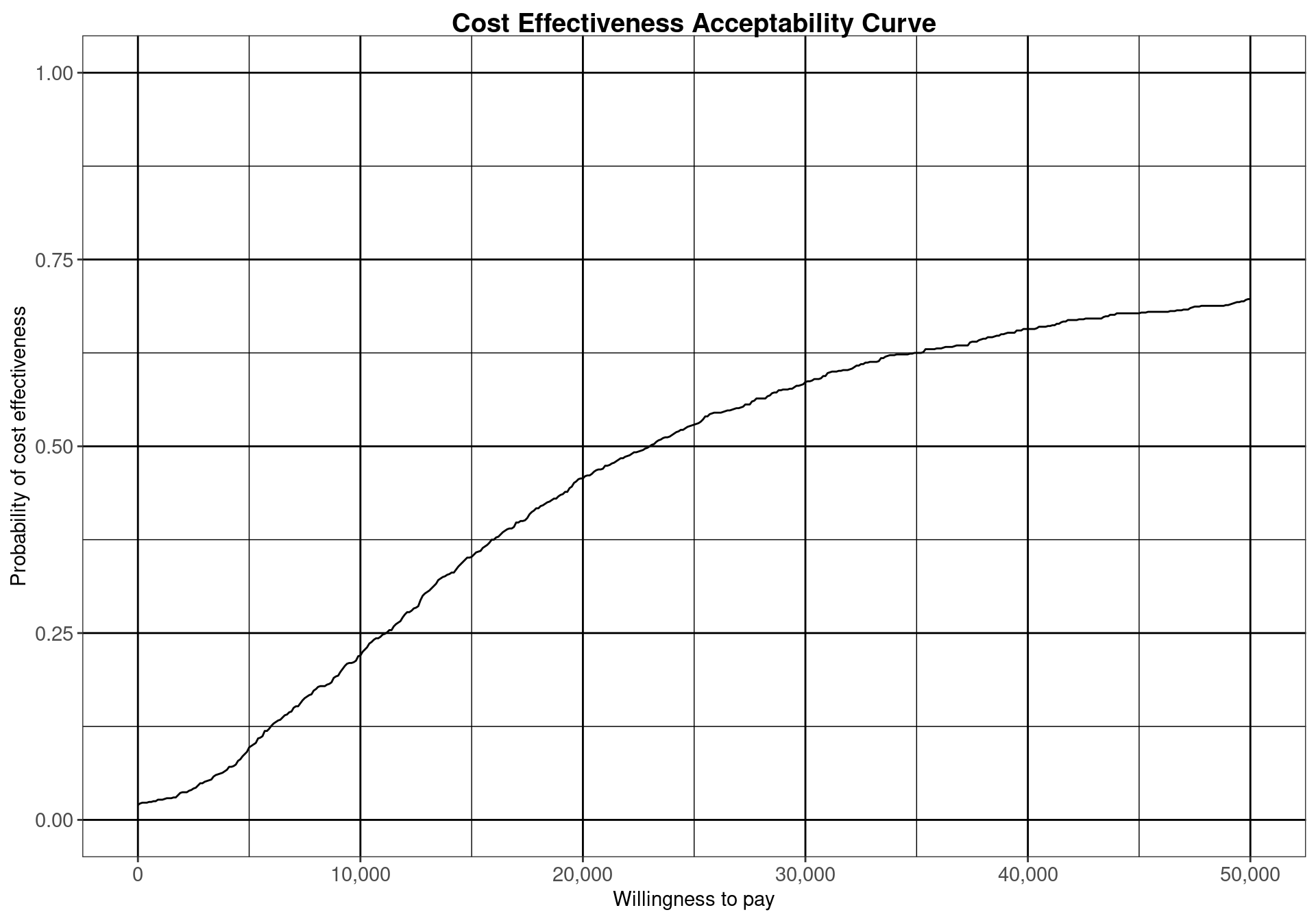
panel.grid in the theme options in ggplot2.
Analysing the CEAC in the interval of willingness to pay values between \(20\,000\) and \(30\,000\) monetary units per QALY demonstrates that this decision is relatively uncertain (notice that depending on the monetary unit selected, the relevant range may vary). The probability of cost-effectiveness for the vaccination strategy compared to the status quo is between \(0.46\) and \(0.59\), close to \(0.50\). For lower thresholds the decision is clearly in favour of not implementing the vaccination, with a CEAC below 0.25 for a willingness to pay threshold less than \(10\,000\) monetary units per QALY. For higher values of willingness to pay, however, the decision uncertainty is still high as the probability of cost-effectiveness does not reach \(0.75\) in the considered range of willingness to pay values.
4.2.2.2 Example: Smoking cessation (continued)
When more than two comparators are considered in an economic analysis, the pairwise CEACs, with respect to a single reference intervention, are calculated by default within the bcea function. For example, Figure 4.7 shows the probability of cost-effectiveness for Group counselling compared to the other interventions in a pairwise fashion. This analysis gives no information about the other comparisons that do not include Group counselling. This can potentially lead to misinterpretations since these probabilities do not take into account the whole set of comparators. This default pairwise analysis is also represented in Figure 3.11, which presents the EIBs compared to Group counselling for the Smoking cessation example. Both these plots less straightforward in the multiple treatment comparison setting as it is unclear how the interventions compare against each other.
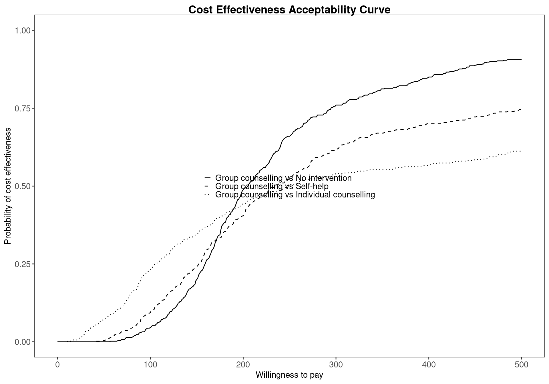
BCEA provides a necessary tool to overcome this problem using the multi.ce function, which computes the probability of cost-effectiveness for each treatment based on the utilities of all the comparators. This allows the user to analyse the overall probability of cost-effectiveness for each comparator, taking into account all possible interventions. To produce a CEAC plot that includes the intervention-specific cost-effectiveness curve, the following code is used. Firstly, the multiple treatment analysis is performed using the bcea object m. The results must then be stored in an mce object. Finally, the plot in Figure 4.8 is produced by calling the ceac.plot function which we’ve met before (previous versions of BCEA used the mce.plot function but this is now deprecated). The argument pos can be used to change the legend position, and in this case it is set to topright to avoid the legend and the curves overlapping.
mce <- multi.ce(m)
ceac.plot(mce, pos="topright")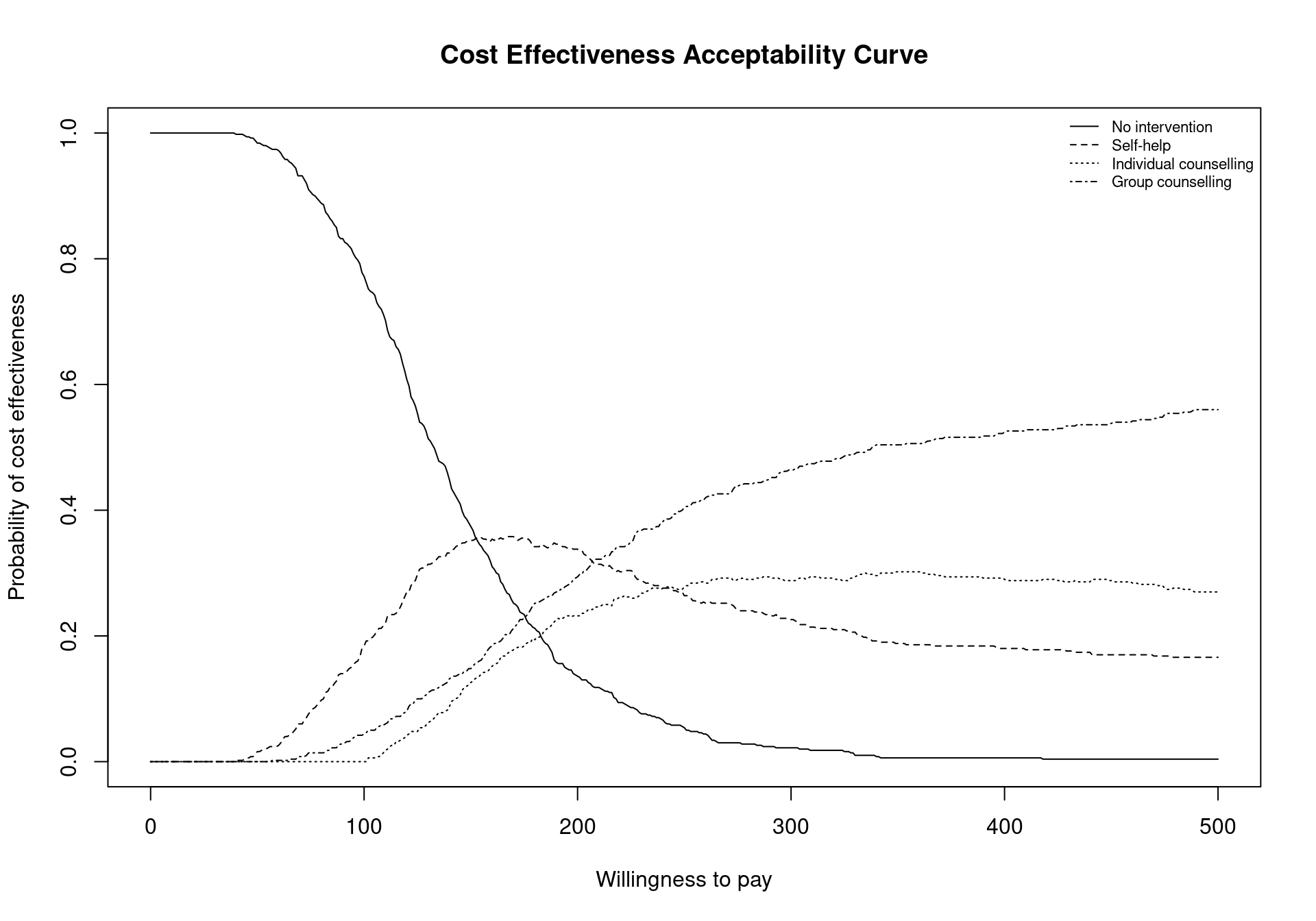
The function multi.ce requires a bcea object as argument. It will output a list composed of the following elements:
m.ce, a matrix containing the values of the cost-effectiveness acceptability curves for each intervention over the willingness to pay grid. The matrix is composed of one row for every willingness to pay value included in thebceaobjectm$k(i.e. 501 if the argumentwtpis not specified in thebceafunction call), and columns equal to the number of included comparators;ceaf, the cost-effectiveness acceptability frontier. This vector is determined by the maximum value of the CEACs for each value in the analysed willingness to pay grid;n.comparators, the number of included treatment strategies;k, the willingness to pay grid. This is equal to the grid in the originalbceaobject, in this examplem$k;interventions, a vector including the names of the compared interventions, and equal to theinterventionsvector of the originalbceaobject.
To produce a graph of the CEACs for all comparators considered together, the command ceac.plot is used. This command accepts as inputs an object produced by the multi.ce function, with the pos argument indicating the legend position. As usual, an option to select whether the plot should be produced using base graphics or ggplot2 can be included. The legend position can be changed in the same way as for the base ceac.plot function Section 3.4.1. Again, if selecting ggplot2, a finer control on the legend’s position is possible. The legend can be placed outside the plot limits using a string providing the position (\(e.g.\) "bottom") or alternatively a two-element vector specifying the relative position on the two axis; the two elements of the vector can assume any value, so that for example c(0.5,0.5) indicates the centre of the plot and c(1,0) the bottom-right corner inside the plot. Line colours and types (e.g., dashed) can be changed by specifying a line list as an additional argument to the ceac.plot function and providing color and type elements. If specified and not matching the number of CEAC curves included in the plot, the first element of the vector will be recycled.
The results displayed in Figure 4.8 confirm and extend the conclusions previously drawn for the Smoking example, No intervention is associated with the highest probability of cost-effectiveness for low willingness to pay thresholds. However, it can also be seen that the probability of cost-effectiveness decreasing steeply as the threshold increases. Between the values \(177\) and \(210\) the curve with the highest value is Self-help but, again, the associated probability of cost-effectiveness is modest, lower than \(0.40\). In addition, it is not substantially higher than the probability of the other interventions being cost effective as the CEAC values are similar.
The values of the CEAC curves can be extracted from the mce object for a given willingness to pay threshold, for example \(194\), using the following code
mce$p_best_interv[which(mce$k==194), ][1] 0.342The code above will return an empty vector if the threshold value \(194\) is not present in the grid vector mce$k. A slightly more sophisticated way of preventing this error is extracting the value in correspondence of the threshold minimising the distance from the chosen threshold, which in this case yields the same output since the chosen willingness to pay is included in the vector.
mce$p_best_interv[which.min(abs(mce$k - 194)), ][1] 0.342A representation of the cost-effectiveness acceptability frontier can also be produced. Within the BCEA package, the frontier is defined as the maximum value of the probability of cost-effectiveness among all comparators for each willingness to pay value. It is an indication of the uncertainty associated with the decision between all the interventions. In other terms, higher frontier values correspond to lower uncertainty. The cost-effectiveness acceptability frontier can also be defined as the probability of cost-effectiveness for the intervention associated with the maximum value for the expected net benefit. In many settings, this will coincide with the intervention with the maximum value for the probability of cost-effectiveness, which is the case for the smoking cessation example, but may not entirely coincide when the probability of cost-effectiveness is very similar between two interventions. Once the multi.ce function has been called, the frontier within BCEA can be easily displayed by the following command, which produces the output in Figure 4.9 (a).
ceaf.plot(mce, graph = "ggplot")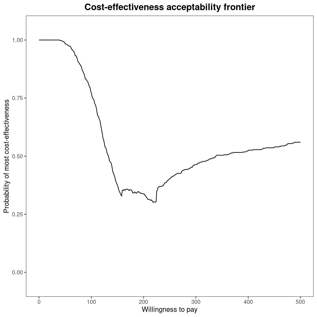
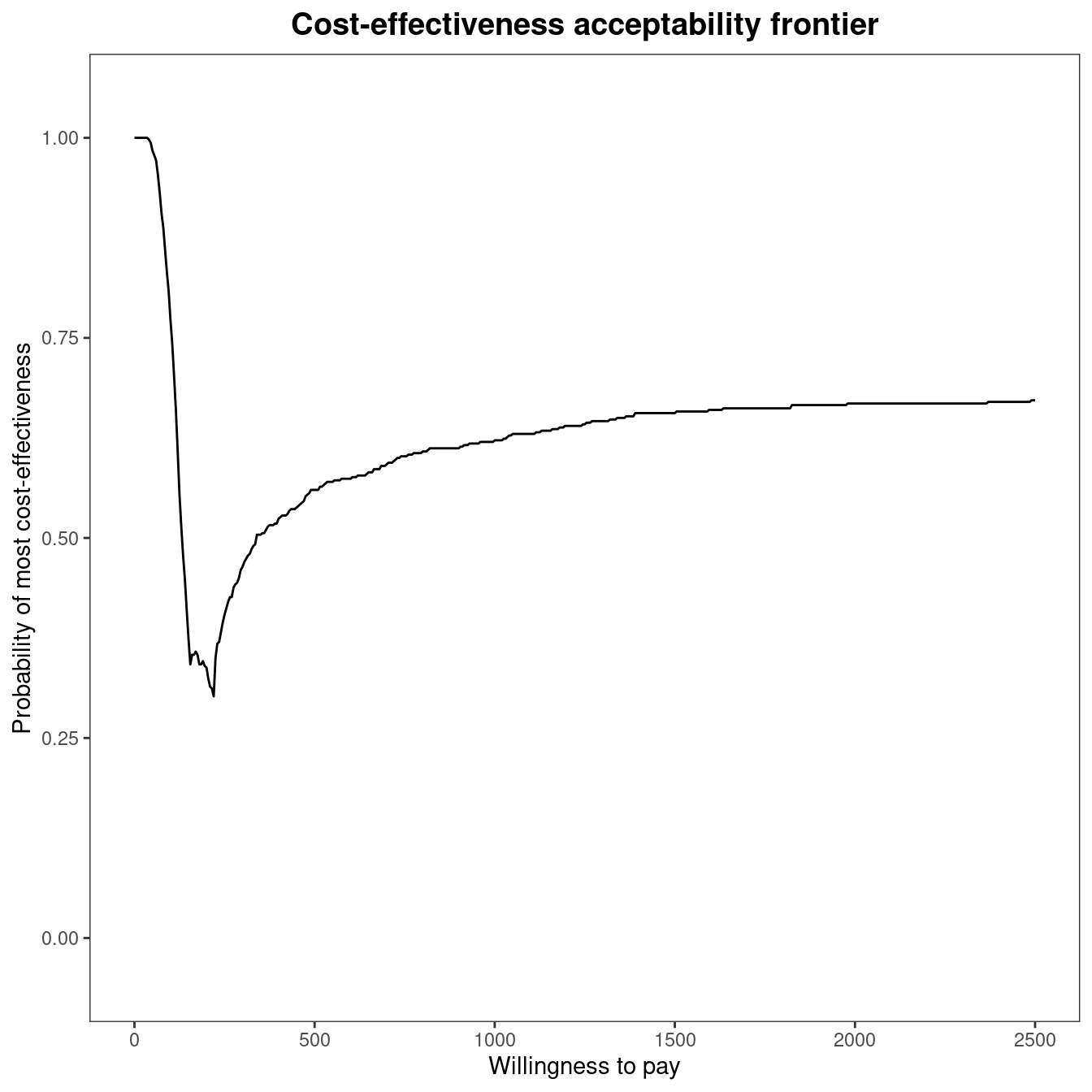
The cost-effectiveness acceptability frontier (CEAF) indicates a high degree of uncertainty associated with the optimality of the decision for willingness to pay thresholds between £150 and £250 per life year gained. The frontier increases in value for increasing thresholds, reaching about 0.60 for a value of £500 per life year gained. This result highlights that, even if Group counselling is the optimal choice for a willingness to pay higher than £200 per life year gained, the associated probability of cost-effectiveness is not very high. Figure 4.9 makes it clear that decision uncertainty does not derive from a comparison with No intervention, which is clearly inferior in terms of expected utilities to the other comparisons. Its associated probability of cost-effectiveness is zero or close to zero for thresholds higher than £350 per life year gained. Therefore, all intervention strategies for smoking cessation are cost-effective when compared to No intervention. The frontier remains stable around a value equal to \(0.60\) for higher thresholds, as shown in Figure 4.9 (b) which plots the frontier for a higher limit of the willingness to pay threshold. To produce this graph, the economic analysis must be re-run as follows:
m2 <- bcea(eff, cost, ref=4, intervention=treats, Kmax=2500)
mce2 <- multi.ce(m2)
ceaf.plot(mce2, graph = "ggplot")
The cost-effectiveness acceptability probability remains stable around a value equal to about \(0.60\), with Group counselling being the optimal choice for willingness to pay values greater than £\(225\) per life year gained.
4.2.2.3 Including the cost-effectiveness frontier in the plot
A small addition to the ggplot2 version of ceac.plot allows for the inclusion of the cost-effectiveness acceptability frontier in the plot. Adding the frontier gives an easier interpretation of the graphical output. There is no built-in option to include it in the graph, but the frontier can be added using the code below.
library(ggplot2)

ceac.plot(mce, graph="ggplot2", pos=c(1,1)) +
  stat_summary(fun=max, geom="line", colour="grey25", alpha=0.3, lwd=2.5)
The code includes some control over the appearance of the frontier in the graph. An additional geom_line layer is added to overlay the cost-effectiveness acceptability frontier, using the aesthetics provided by the ceac.plot function. The values of the curve over the willingness to pay grid are calculated by means of the stat_summary function using maximum value of the curves on each point. Figure 4.10 demonstrates the produced graphic.
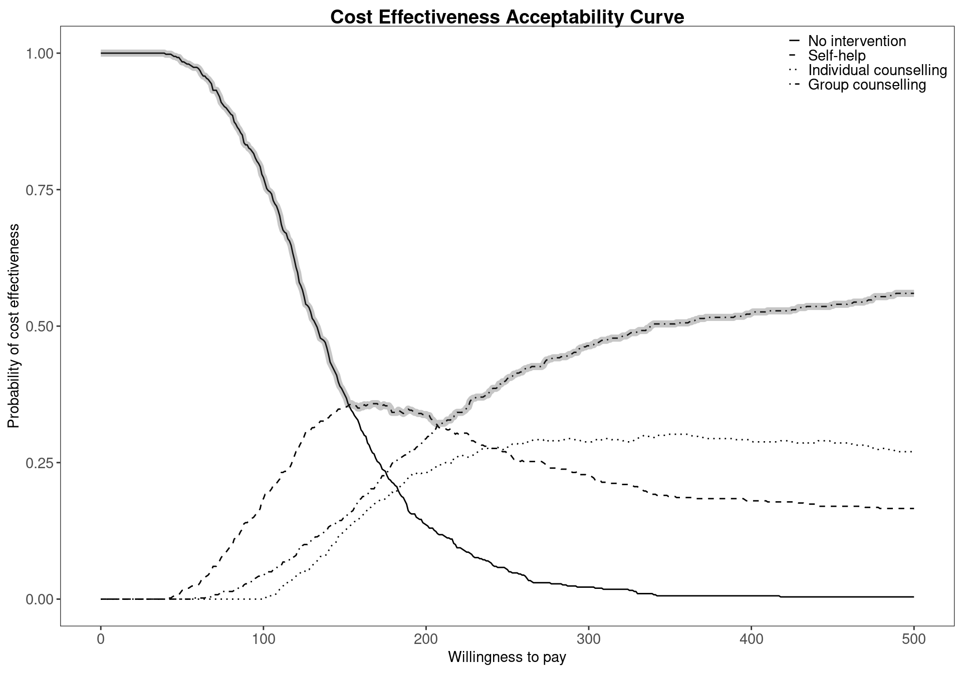
alpha available in the geom_line layer makes it easy to understand graphically which comparator has the highest probability of cost-effectiveness.
4.3 Value of Information Analysis
As already introduced in Section 4.1, PSA can be undertaken to ascertain whether it is worth gathering additional information before deciding whether to reimburse a new treatment. In a fully Bayesian setting, new evidence about the model parameters is easily integrated with the currently available information using Bayes Theorem. In fact, this new information updates the posterior distributions for the model parameters, which in turn feed into the economic model and updates the cost and effectiveness measures (see Figure 1.5). In most settings, this new information about the statistical model will reduce our decision uncertainty and reduce the risk of decision makers funding an inefficient treatment. Thus, the new information reduces the chance that an intervention that is optimal based on current evidence is, in fact, non-optimal in reality. As the implementation of a non-optimal intervention inevitably comes with the societal cost, which can be measured as the difference between the value of the true optimal intervention and the implemented intervention, the collected information can be said to be valuable if it prevents this waste of resources.
However, collecting additional information also comes at a cost, which is the cost of data collection, \(e.g.\) the cost of a further clinical trial. Therefore, we want to assess whether the potential value of additional information exceeds the cost of collecting this information. This will come down to two components, the probability of funding the incorrect treatment if the decision is based on current evidence, represented by the CEAC, and the potential cost of funding a non-optimal treatment. We refer the reader to Heath et al. (2024) and Heath et al. (2025) for much more detailed information on both the methodological and computational recent advances in the application of Value of Information analysis, specifically in Health Technology Assessment.
4.3.1 Expected value of perfect information
One measure to quantify the value of additional information is known as the Expected Value of Perfect Information (EVPI). When used to compute the value of information based on a health economic decision model that uses a net monetary benefit utility function, i.e., the standard setting in BCEA, it computes the value of eliminating parameter uncertainty in monetary units. The exact monetary units (for example, pounds, dollars, euros, etc) will depend on the monetary units used to specify the costs in the health economic model. The EVPI is based on the Opportunity Loss (OL), which measures the potential losses associated with choosing the most cost-effective intervention on average when it does not result in the intervention with the highest net benefit in a “possible future”. These “possible futures” can be thought of as obtaining enough relevant data to know the exact value of the net benefit for each of the different interventions and therefore decision makers to known the optimal treatment with certainty.
To calculate the EVPI practically, possible futures depend on the parametric uncertainty defined for each of the model parameters and the different net benefits are calculated through simulation. This is exactly the process of PSA as the net benefit, conditional on a fixed willingness-to-pay threshold, is computed for a large number of simulated parameter values. To compute EVPI, we assume that the net benefit values in each simulation are known and correspond to a possible future. This means that the distribution for the net benefits across all potential futures is induced solely by parameter uncertainty. The opportunity loss, used to compute EVPI, is the difference between the maximum value of the simulation-specific (known-distribution) utility \(U^*(\pmb\theta)\) and the utility for the intervention resulting in the overall maximum expected utility \(U(\pmb\theta^\tau)\), where \(\tau=\text{arg max}_t ~\mathcal{U}^t\) (see the discussion in Section 4.2.1): \[ \text{OL}(\pmb\theta) = U^*(\pmb\theta) - U(\pmb\theta^\tau). \tag{4.1}\]
The OL will be 0 when the optimal treatment on average is also the optimal treatment for that specific simulation. In this way, the distribution of the OL is related to the CEAC as the probability that the OL is 0 is equal to the CEAC for the optimal intervention. When the OL is non-zero, it will be positive as either we choose the current optimal treatment or the treatment with a higher utility value for that specific simulation. Revisiting the simulation table for the Vaccine example,
data(Vaccine)
treats <- c("Status quo", "Vaccination")
m <- bcea(eff, cost, ref=2, interventions=treats)
table <- sim_table(m, wtp=25000)
head(table$Table)
U1 U2 U* IB2_1 OL VI
1 -36.57582 -38.71760 -36.57582 -2.1417866 2.141787 -1.750121
2 -27.92514 -27.67448 -27.67448 0.2506573 0.000000 7.151217
3 -28.03024 -33.37394 -28.03024 -5.3436963 5.343696 6.795451
4 -53.28408 -47.13734 -47.13734 6.1467384 0.000000 -12.311646
5 -43.58389 -40.40469 -40.40469 3.1791976 0.000000 -5.578996
6 -42.37456 -33.08547 -33.08547 9.2890987 0.000000 1.740230we can see that the OL is equal to 0 when the incremental benefit is positive and equal to the absolute value of the incremental benefit when the incremental benefit is negative.
The EVPI is then defined as the average of the opportunity loss. This measures the average potential losses in net benefit that would be incurred if the current optimal intervention was implemented. Thus, EVPI is driven by the simulations in which the simulation specific optimal decision is non-optimal in expectation, which is related to the CEAC but includes an additional element that accounts for the OL when the intervention in non-optimal. \[\begin{align} \text{EVPI} = \mbox{E}[\text{OL}(\pmb\theta)] \end{align}\] If the probability of cost-effectiveness is low then more simulations will give a non-zero OL and consequently the EVPI will be higher. Conversely, if the probability of cost-effectiveness is very high, it is unlikely that more information would be worthwhile, as the most cost-effective treatment is already evident. However, there may be settings where the probability of cost-effectiveness is low, so the decision maker believes that decision uncertainty is important. However, this could simply be because the two treatments are very similar in both costs and effectiveness. In this case the OL would be low as the net benefit values are similar for both treatments for all simulations. Therefore, the OL of making the incorrect decision is very low. This will be reflected in a low value for EVPI but will not be evident from the CEAC, potentially leading to decision makers placing undue importance on reducing the decision uncertainty before making a decision. This is because, for low EVPI value, the optimal treatment can be chosen with little financial risk, even with a low probability of cost-effectiveness.
Finally, note that the definition of EVPI given here does not change irrespective of the number of interventions included in the decision model. This is because OL is always defined across all the interventions included in a decision models, implying that, in contrast to the CEAC, it is not possible to compute the “pairwise” EVPI.
4.3.1.1 Example: Vaccine (continued)
To give an indication of the cost of uncertainty for a chosen value of \(k\), the EVPI is presented in the summary table. For the Vaccine example, this measure is estimated to be equal to \(£2.41\) for a threshold of \(£25,000\) per QALY. Despite the advantages of EVPI, one drawback is that the interpretation of the EVPI is more challenging than the CEAC as it is an unbounded measure. While it is simple to state that value of the CEAC close to 1 or 0 indicate a low level of decision uncertainty, these rules of thumb are not readily available for EVPI.
To determine whether EVPI indicates a “high” or “low” level of decision uncertainty, we remember that EVPI can also be thought of as the expected value of learning the true values of all the model parameters underlying the health economic model. In general, information about model parameters is obtained through a research study, \(e.g.\) a clinical trial, a literature review or an observational study. So, while these proposed research studies are not able to learn the exact values of all model parameters, EVPI can be thought of as an upper bound for all future research costs. This is because EVPI is the maximum possible value that could be achieved through any proposed research study. Thus, if the costs associated with additional research exceed the EVPI then the decision should be made under current information. This allows us to interpret EVPI by comparing it with the cost of research.
For this example, EVPI is \(£2.41\) for a threshold of \(£25,000\) per QALY. As is standard in BCEA for a health economic model that computes the per person benefit of each intervention, the provided EVPI value is the per person EVPI. To compare with the cost of future research this EVPI value should be multiplied by the number of people who will receive the treatment. This is because the cost of an incorrect decision is higher if a greater number of patients use the treatment. As vaccines are typically implemented across the whole population, decisions around the implementation of a influenza vaccine will typically affect a large number of individuals, \(\approx 67\) million in the UK. This EVPI value multiplied by the number of individuals affected by the decision will exceed \(£160\) million, which clearly substantially exceeds the cost of any additional research strategy. Therefore, this analysis implies that there is potentially value in collecting additional information before implementing the Vaccination strategy. While this conclusion emphasises the importance of collecting additional information, similar to the CEAC values in Section 4.2.2.1, there are often settings where the conclusions about decision uncertainty based on the CEAC are different from those made based on EVPI.
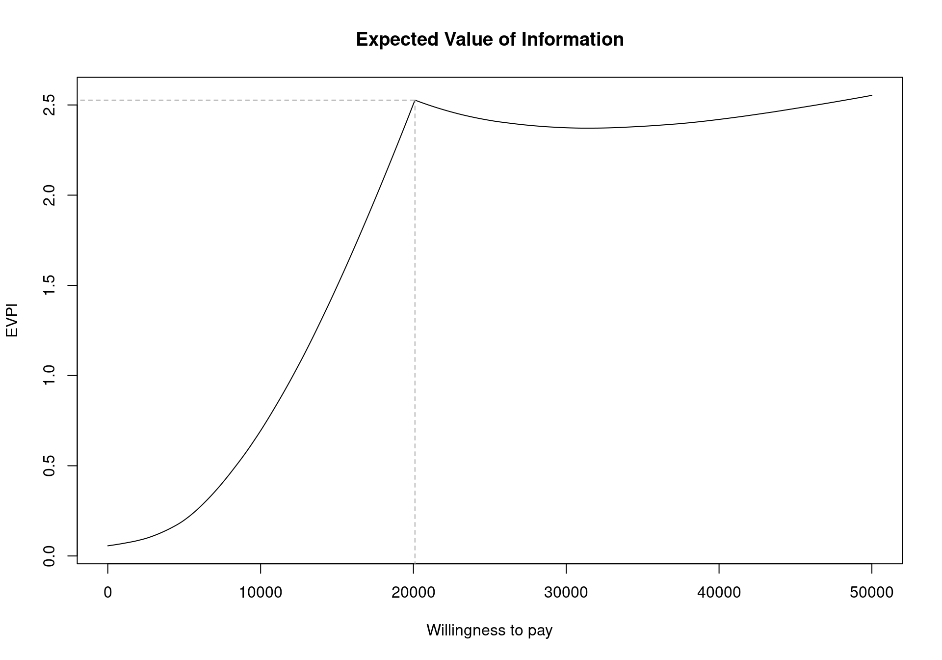
The EVPI can be easily analysed over different willingness to pay values using BCEA. To represent the curve graphically, the function evi.plot is used. This function uses the bcea object m, and produces the plot of the EVPI over the willingness to pay grid of values m$k. To produce the output in Figure 4.11, it is sufficient to execute the following code:
evi.plot(m)The analysis of EVPI over different willingness to pay values highlights an increase in the value of information until the break-even point, at \(20\,100\) monetary units. The break-even point is where the uncertainty associated with the decision reaches a local maximum value. The EVPI then increases as the willingness to pay increases because the opportunity loss is related to the net benefit which increases as the willingness to pay is increases. Again, these plotted values represent the per person EVPI, while evaluating whether this represents a “high” value of information should be evaluated based on the population-level EVPI. Another consideration for the population-level EVPI is whether the intervention will be used by future patients. In this analysis, we assume that there will be single vaccination campaign but different diseases will require more complex evaluations of the number of individuals to benefit from an intervention (Philips et al., 2008).
4.3.1.2 Example: Smoking cessation (continued)
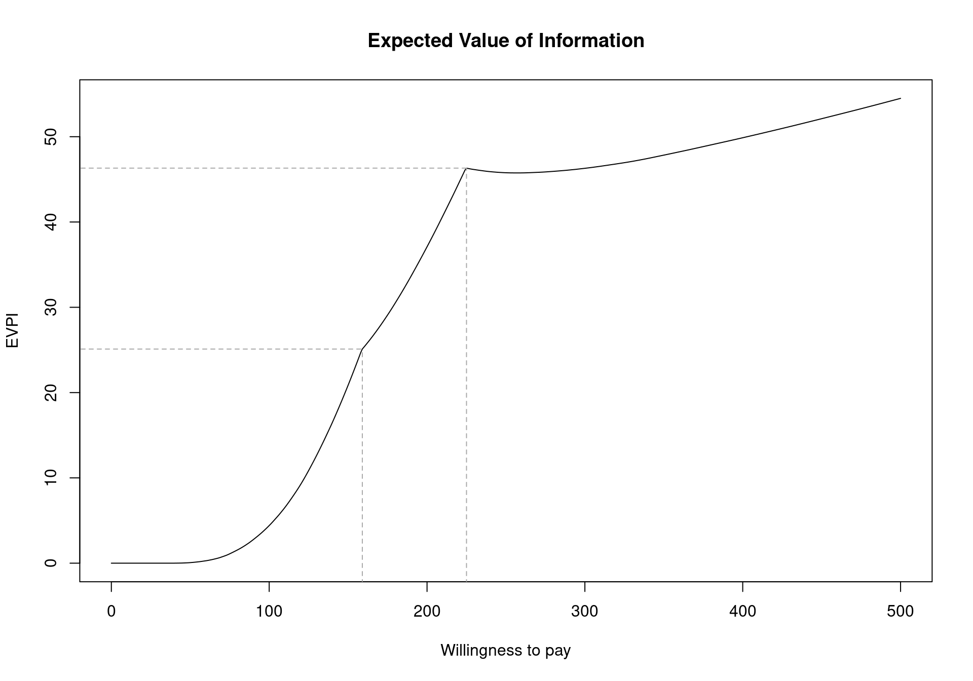
The analysis of the expected value of information can be carried out for multiple comparators in the same way. Once the bcea object m is obtained, the EVPI can be plotted using:
evi.plot(m)As already presented in Section 4.2.2.2, the two break-even points can be seen in Figure 4.12 as inflection points: the first one when the decision changes from implementing “No treatment” to “Self-help” (\(k_1^*=\)£177) and the second when the optimal decision changes to “Group counselling” (\(k_2^*=\)£210). Notice that, as discussed earlier, the EVPI is a single value even in the multi-comparison setting. This is in contrast to all the other measures that must be extended in the multi-comparison setting and happens because the EVPI is based on the average opportunity loss across all the possible treatment options. For example, while Group Counselling dominates on average for larger willingness to pay values, the dominating treatment for a specific simulations can be either No treatment, Individual Counselling or Self-Help. This induces one value for the opportunity loss for each simulation, rather than three different values.
The cost-effectiveness frontier, in Figure 4.10, showed that the probability of cost effectiveness rapidly decreases as the willingness to pay increases from 0 before stabilising below \(0.60\) for willingness to pay values greater than £150. Therefore, there is a moderate amount of uncertainty about which treatment is cost effective. However, Figure 4.12 shows that the per-person EVPI is relatively low. Additionally, the population of individuals who make use of smoking cessation services each year is substantially below the total UK populations. As such, depending on the this number, it may be possible that the population-level EVPI does not substantially exceed reasonable study costs. In this setting, we should proceed with Group Counselling without performing additional research. Again, this highlights the importance of the EVPI as a tool for PSA as it takes into account both the opportunity loss and the probability of making an incorrect decision.
Again, it is important to emphasise that the population-level EVPI must be compared with the costs of future research for the specific decision problem under consideration. While the value of resolving the uncertainty in the health economic model may seem high, the costs of research are also often substantial and EVPI must be interpreted in the context of the modelling scenario, not against a general purpose threshold or comparator.
4.3.2 Expected Value of Perfect Partial Information
EVPI is a useful measure as it can be easily computed from the results of a standard PSA procedure. Thus, it can be calculated alongside the CEAC as part of a BCEA standard procedure. This allows both the CEAC and the EVPI to be provided as part of the general plot and summary functions. However, in the case where the EVPI is high compared to the cost of additional research it is useful to know where to target that research to reduce the decision uncertainty sufficiently. In addition to this, it is often important to identify the parameters that are driving uncertainty in decision making as this allows decision makers to focus on the key elements of uncertainty in the model. From a research design or prioritisation perspective, identifying the drivers of decision uncertainty also allows research to determine which research studies would reduce uncertainty the most efficiently. This ensures that, having postponed the decision between different interventions, we are able to provide the cost-effective intervention to patients as soon as possible.
This analysis of the drivers of decision uncertainty is very important in health-economic modelling as some of the underlying parameters are known with relative certainty. For example, there may be large amount of research on the prevalence of a given disease or the prevalence is estimated from a population-level database; similarly, the cost of the treatment may be known with reasonable precision. Evidently, investigating these parameters further to reduce the decision uncertainty would waste valuable resources and delay getting a potentially cost-effective intervention to market. Ideally, therefore, it would be advisable to calculate the value of resolving uncertainty for certain parameters or subsets of parameters in order to target research efforts and understand the drivers of model uncertainty.
This subset analysis would also be important in prioritising a specific proposed research study. In this setting, the proposed study should target those model parameters that are associated with high value. Even further, we can compare the value of learning specific model parameters with the cost of the proposed study to provide additional information for these parameters. Again, if the value of the parameters is less than the cost of future research, these parameters should be excluded from future research as sufficient evidence is available for decision making.
In general, the value of a subset of parameters is known as the Expected Value of Perfect Partial Information (EVPPI); this indicator quantifies the value of learning the exact value of a specific parameter (or subset of parameters), while remaining uncertain about the remaining model parameters. While intuitively this is appears a simple extension to the general framework in which the EVPI is computed, the quantification of the EVPPI does pose serious computational challenges. Traditionally, the EVPPI was calculated using computationally intensive nested simulations. However, algorithms have been developed Heath et al. (2017) that allow users to approximate the EVPPI efficiently.
Crucially, these approximation methods for EVPPI are based solely on the PSA values for the parameters (\(e.g.\) in a Bayesian setting the posterior distribution obtained using MCMC methods), allowing these methods to be included in general purpose software like BCEA. To begin, the PSA value for the parameters themselves need to be stored and loaded in R. These PSA samples must be the parameter simulations used to calculate the measures of costs and effectiveness. In a Bayesian setting these will typically be available in a BUGS/JAGS object in R as in Section 4.3.3.4). However, if the health economic model has been built in Excel then the parameter simulations can be loaded into R from a .csv file to calculate the EVPPI (see Figure 5.5 and the discussion in Section 5.2.6.1 and Section 5.2.7). For example, if a spreadsheet containing simulated values for a set of relevant parameters was saved as the file PSAsimulations.csv, then these could be imported in R using the commands
psa_samples <- read.csv("PSAsimulations.csv", header=TRUE)The resulting object psa_samples could then be passed to BCEA to execute the analysis of the EVPPI.
4.3.3 Approximation Methods for the computation of the EVPPI
Broadly, the goal of the approximation methods discussed in this section and implemented in BCEA is to speed up computation (allowing for feasible EVPPI estimates) and the standardise the calculation method so it can be made available in software. The following section gives a short introduction to the theoretical background required for these estimation methods. This background will help readers to understand the more advanced options presented in Section 4.3.4. However, the EVPPI can be calculated with BCEA without using these more advanced options and readers can proceed directly to Section 4.3.3.4, which presents an example of EVPPI calculation.
Before discussing the approximation methods, we formalise the definition of EVPPI. As discussed, EVPPI quantifies the impact of uncertainty in a specific subset of parameters of interest on the decision-making process. We denote the parameter subset of interest as \(\pmb\phi\) and we denote all remaining parameters in the model as \(\pmb\psi\). In other words, we split the complete set of parameters into \(\pmb\theta=(\pmb\phi,\pmb\psi)\), where \(\pmb\psi\) are “nuisance” parameters for the purpose of EVPPI calculation. For example, with reference to the Vaccine example (see Section 2.3.1), we could define the parameters of interest \(\pmb\phi=(\beta_j,\gamma_2,\xi,\lambda)\) and \(\pmb\psi\) as all remaining parameters in the model.
From the theoretical point of view, the procedure used to define the EVPPI closely mimics the one used for the EVPI. However, the opportunity loss is computed only after the uncertainty due to limited knowledge of \(\pmb\psi\) is averaged out. In this case, the opportunity loss is the cost of selecting the treatment that is considered to be optimal on average given current evidence when it is less cost-effective than its comparator(s) in some “potential futures”, where the potential futures defined by knowing the exact value of the parameters \(\pmb\phi\). Therefore, to define EVPPI, we must calculate the value of the optimal treatment conditional on a known value of \(\pmb\phi\) and after the uncertainty due to \(\pmb\psi\) has been marginalised out: \[ \begin{aligned} U^*(\pmb\phi) & = \max_t E_{\pmb\psi\mid\pmb\phi}\left[ E_{(e,c)\mid\pmb\theta} \left[u(e,c;t)\right] \right] \\ & = \max_t E_{\pmb\psi\mid\pmb\phi} \left[ g_t(\pmb\theta) \right]. \end{aligned} \tag{4.2}\]
In line with Equation 4.1, the opportunity loss for a specific value \(\pmb\phi\) is the difference between the value \(U^*(\pmb\phi)\) and the utility for the intervention resulting in the overall maximum utility \[ \text{OL}(\pmb\phi) = U^*(\pmb\phi) - U(\pmb\phi^\tau), \] where \(U(\pmb\phi^\tau)\) is the utility for the overall optimal intervention with uncertainty due to \(\pmb\psi\) marginalised out. Finally, the EVPPI is the expectation of this (conditional) opportunity loss \[ \begin{aligned} \mbox{EVPPI} & = E_{\pmb\phi}[\text{OL}(\pmb\phi)] \\ & = E_{\pmb\phi}[U^*(\pmb\phi)] - \mathcal{U}^*. \end{aligned} \]
This formulation adds very little theoretical complexity, with respect to the EVPI. However, the calculation of \(U^*(\pmb\phi)\) involves a maximisation over a conditional expectation, which greatly complicates the computation using the default simulation-based method. This is because the conditional expectation of the net benefit for each value of \(\pmb\phi\) would need to be estimated using a large number of simulations. This requires a nested simulation procedure where a complete PSA must be run for each simulated value of \(\pmb\phi\) in the original PSA. Furthermore, EVPPI can be computed for different subsets for \(\pmb\phi\), requiring even more computational burden compared to computing EVPI. Finally, the original PSA simulations alone cannot be used directly the calculate the EVPPI as additional simulations from the conditional distribution of the parameters must be obtained to appropriately compute the conditional exception. Thus, the general purpose simulation-based method for EVPPI is computationally expensive and requires that the health economic decision model is rerun many times.
Consequently, approximation methods were developed to approximate the conditional expectation as efficiently as possible, based solely on the PSA simulations. While a range of methods have been developed for single and multi-parameter subsets, the most widely applicable method (Heath et al., 2017) uses regression to approximate the function \(g_t(\pmb\phi)\) (Strong et al., 2014), where \[ g_t(\pmb\phi) = E_{\pmb\psi\mid\pmb\phi} \left[U_t(\pmb\theta) \right], \] for each treatment option \(t\). This method uses regression to marginalise out the uncertainty due to the nuisance parameters \(\pmb\psi\). Crucially, once the function \(g_t(\pmb\phi)\) has been estimated for all treatment options then \(U^*(\pmb\phi)\) can be easily approximated using \[ U^*(\pmb\phi) = \max_t g_t(\pmb\phi). \]
As demonstrated in Strong et al. (2014), regression can be used to marginalise out uncertainty due to \(\pmb\psi\) by noting that the observed utility values \(U_t(\pmb\theta)\) from the PSA analysis can be thought of as a set of “noisy” observations of the function \(g_t(\pmb\phi)\): \[ \begin{aligned} U_t(\pmb\theta) & = E_{\pmb\psi\mid\pmb\phi}\left[U_t(\pmb\theta)\right] + \varepsilon \\ & = g_t(\pmb\phi) + \varepsilon, \nonumber \end{aligned} \tag{4.3}\] assuming that \(\varepsilon \sim \mbox{Normal}(0,\sigma_\varepsilon^2)\). In Equation 4.3, the computed values of \(U_t(\pmb\theta)\), which are available from the PSA process described in Section 4.2.1, are used as the response variable in the regression, and the simulated values of the parameters of interest as used as the “covariates” or independent variables. Both these quantities are extracted from the simulations required for PSA and therefore available at no extra computational cost, once the PSA procedure is in place.
Notice that in Equation 4.3, the target to be estimated is the unobserved maximum conditional expectation \(E_{\pmb\psi\mid\pmb\phi}\left[U_t(\pmb\theta)\right]\), which is effectively a function of \(\pmb\phi\) only, which we indicate as \(g_t(\pmb\phi)\). This is because uncertainty due to other parameters has been marginalised out leaving a function conditional on the values of \(\pmb\phi\) only. In general, this function \(g_t(\pmb\phi)\) can have a complicated form implying that a method such as linear regression would be unlikely to capture the relationship between \(\pmb\phi\) and \(E_{\pmb\psi\mid\pmb\phi}\left[U_t(\pmb\theta)\right]\). Therefore, a flexible regression method is needed, to estimate function \(g_t(\pmb\phi)\). A possible way of doing this is to use “non-parametric” regression methods, in which the predictor does not take a predetermined form but is constructed according to information derived from the data. Once the function \(g_t(\pmb\phi)\) has been estimated, it is possible to use the resulting estimates to find the average opportunity loss as all the other terms can be simply calculated directly from the health-economic model output.
By default, the BCEA function evppi uses Generalised Additive Models (GAM) (Hastie and Tibshirani, 1990) when \(\pmb\phi\) contains four parameters or fewer; we briefly describe this in Section 4.3.3.1. For the general case in which \(\pmb\phi\) contains more than four parameters, bcea resorts to a fast Gaussian Process (GP — Rasmussen and Williams, 2006) approximation method developed for EVPPI calculation in Heath et al. (2016), which we present in Section 4.3.3.3. In some settings, this fast approximation method will not be sufficient and the evppi function can also implement a GP regression method described by Strong et al. (2014) and discussed in Section 4.3.3.2 below. While this is in some cases slightly more flexible (because of its underlying formulation), it is in general less efficient from the computational point of view.
The following sections give a short explanation of all these methods in order that the user may have a fuller understanding of the technical, regression method specific aspects that can be manipulated by the user in BCEA. We note that the complexity of the mathematical formulation is beyond the scope of this book and thus we only sketch the basic features of the advanced methods. The reader is referred to the relevant literature for more in-depth information.
4.3.3.1 Generalised additive models
GAMs model the observed net benefit values as a sum of smooth functions of the important parameters \(\pmb\phi\). In BCEA, these smooth functions are splines — technically these are piecewise polynomial functions where the degree of the polynomial defines the smoothness of the function. The polynomial degree is selected automatically by the evppi function. This effectively amounts to modelling \[
g_t(\pmb\phi_s) = \sum_{q=1}^{Q_\phi} h_t(\phi_{s,q}),
\] where \(Q_\phi\) is the number of important parameters (i.e. the size of the subset \(\pmb\phi\)), \(h_t(\cdot)\) are the smooth functions, \(\pmb\phi_s\) is the \(s\)-th simulated value of the \(\pmb\phi\) vector from the PSA and \(\pmb\phi_{s,q}\) is the \(s\)-th simulated value of the \(q\)-th element of the \(\pmb\phi\) vector from the PSA.
In standard GAM regression methods, each smooth function or spline is a function of one parameter in the set \(\pmb\phi\). This can occasionally be too restrictive in health-economic models, especially when the values in \(\pmb\phi\) are correlated and/or interact in the net benefit function. Thus, the EVPPI estimate that uses univariate splines is unreliable. It is for this reason that for multi-dimensional vectors of \(\pmb\phi\) a different regression method is used by default in evppi function. In this case, evppi uses a GAM that includes all possible interactions between the parameters in \(\pmb\phi\). This means that the polynomials include cross terms and therefore the number of terms in the spline model is greatly increased, especially for parameter subsets that include a higher number of parameters. For example, the default spline choice within the evppi function (cubic splines) would require 125 parameters when \(Q_\phi=3\).
While the estimation procedure is still extremely fast, a large dataset (i.e. \(S=50,000\)) is required to calculate the EVPPI when \(\pmb\phi\) contains more than 4 parameters. Additionally, even a large dataset cannot prevent over-parametrisation in some settings meaning that the GAM cannot fitted accurately. It is possible to remove these interaction terms in BCEA, as shown in Section 4.3.4 but, again, this can negatively effect the accuracy of the estimate.
4.3.3.2 “Standard” Gaussian Process regression
As suggested by Strong et al. (2014), one way to overcome the limitations of GAMs is to use GP regression to estimate the conditional expectation of the utility value (Equation 4.2). This strategy effectively amounts to modelling the observed utility values, \(i.e.\) the regression “response” \(U_t(\pmb\theta)\) as a multivariate normal \[ \left( \begin{array}{c} U_t(\pmb\theta_1)\\ U_t(\pmb\theta_2)\\ \vdots\\ U_t(\pmb\theta_S) \end{array} \right) \sim \mbox{Normal}(\pmb H \pmb\beta, \pmb\Sigma + \sigma_\varepsilon^2\pmb I), \tag{4.4}\] where \(\pmb\theta_s\) and \(\pmb\phi_s\) are the \(s\)-th simulated value for \(\pmb\theta\) and \(\pmb\phi\), respectively, \(\sigma_\varepsilon^2\) is the residual variance from the regression construction, \(\pmb H\) is a design matrix \[ \pmb H =\left( \begin{array}{c c c c} 1 & \phi_{11} & \cdots & \phi_{1Q_{\phi}}\\ 1 & \phi_{21} & \cdots & \phi_{2Q_{\phi}}\\ \vdots& & \ddots\\ 1 & \phi_{S1} & \cdots & \phi_{SQ_{\phi}}\\ \end{array}\right); \tag{4.5}\]
\(\pmb\beta\) is the vector of regression coefficients describing the linear relationship between the important parameters \(\pmb\phi\) and the conditional expectation of the net benefits. This means that the mean utility value is based on a linear regression of \(\pmb\phi\). However, a GP is more flexible than linear regression due to the covariance matrix \(\pmb\Sigma\), which is determined by a covariance function \(\pmb{\mathcal{C}}\), a matrix operator whose elements \(\mathcal{C}(r,s)\) describe the covariance between any two points \(U_t(\pmb\theta_r)\) and \(U_t(\pmb\theta_s\)).
Strong and Oakley’s original formulation uses a squared exponential covariance function \(\pmb{\mathcal{C}}_{\textrm{Exp}}\), defined by \[ \mathcal{C}_{\textrm{Exp}}(r,s) = \sigma^2 \exp\left[\sum_{q=1}^{Q_\phi} \left(\frac{\phi_{rq}-\phi_{sq}}{\delta_q} \right)^2\right] \tag{4.6}\] where \(\phi_{rq}\) and \(\phi_{sq}\) are the \(r\)-th and the \(s\)-th simulated value of the \(q\)-th parameter in \(\pmb\phi\), respectively. For this covariance function, \(\sigma^2\) is the GP marginal variance and \(\delta_q\) defines the “smoothness” of the relationship between two utility values with “similar” values for \(\pmb\phi_q\). For high values of \(\delta_q\) the correlation between the two conditional expectations with similar values for \(\phi_q\) is small. Therefore, the function \(g_t(\pmb\phi)\) is a very rough (variable) function of \(\pmb\phi_q\). The \(\delta_q\) values are treated as hyperparameters to be estimated from the data.
This model includes \(2Q_\phi+3\) hyperparameters: the \(Q_\phi+1\) regression coefficients \(\pmb\beta\), the \(Q_\phi\) “smoothness” parameters \(\pmb\delta=(\delta_1,\ldots,\delta_{Q_\phi})\), the marginal standard deviation of the GP \(\sigma\) and the residual error \(\sigma_\varepsilon\) of Equation 4.3. The multivariate normal structure allows the use of numerical optimisation to find the maximum a posteriori estimates for these hyperparameters. This however implies a large computational cost (Heath et al., 2017) — technically, the reason is the necessity to invert a large, dense matrix (that is a matrix full of non-zero entries). This means that while extremely flexible, because there is a specific parameter \(\delta_q\) for each of the elements in \(\pmb\phi\), the resulting estimation can be very computational intensive.
4.3.3.3 Gaussian Process regression based on INLA/SPDE
To overcome the computational complexity of the standard GP regression method, it is possible to set up the problem in a more complex manner, which nonetheless has the advantage of employing computational tricks to speed up the process of hyperparameter estimation by a considerable margin. Specifically, it reduces the additional computational complexity involved wen adding more parameters to \(\pmb\phi\). The basic model can be reformulated (Heath et al., 2016) to make use of a fast approximate Bayesian computation method known as the Integrated Nested Laplace Approximation (INLA) (Rue et al., 2009) to obtain the posterior distributions for the hyperparameters and estimate the function \(g_t(\pmb\phi_s)\).
In a nutshell (and leaving aside all the technical details, which are beyond the scope of this book), the idea is to modify model Equation 4.4 so that the unknown functions \(g_t(\pmb\phi)\) are estimated as a function of a linear predictor \(\pmb H \pmb\beta\), which includes the impact of all the parameters in \(\pmb\phi\), and a “spatially structured” effect \(\pmb\omega\), which effectively takes care of the non-linearity and the correlation among the parameters — performing the same role as the covariance matrix.
Crucially, it is possible to apply the Stochastic Partial Differential Equation (SPDE) method developed in (Lindgren et al., 2011) in combination with the INLA procedure to estimate all the relevant quantities using a “surface” that approximates the impact of the covariance matrix at each point in the parameter space, without explicitly including the \(\delta_q\) parameters. Although this surface theoretically exists for all points in the parameter space \(\pmb\phi\), it is only evaluated at a finite set of points on an irregular grid. The value of the surface at points not on the grid is estimated by interpolation. This is a very fast and efficient procedure.
If the grid points are too far apart then the estimation quality is limited as the surface will not capture all the information about the covariance matrix. However, as the computational time is linked to the number of grid points, fewer grid points will decrease the computational time. The evppi function creates the grid automatically but to increase computational time or accuracy this grid can be manipulated, as we show in Section 4.3.5.
This grid is only computationally efficient in 2-dimensions so dimension reduction is used to obtain a suitable 2-dimensional transformation of the parameters to estimate covariance matrix. This dimension reduction, known as Principal Fitted Components, tests whether these 2 dimensions contain all the relevant information about the utility values. Therefore, if this test indicates that more than 2 dimensions are needed to contain all the information then this method can struggle and full residual checking is required to check the estimation procedure, see Figure 4.15 and Figure 4.16.
Before showing how BCEA can be used to compute the EVPPI, we mention that in order to do so, it is necessary to install the R packages INLA and splancs. As usual, this can be done by typing to the R terminal the following commands.
install.packages("splancs")
install.packages(
   "INLA",
   repos=c(getOption("repos"),
   INLA="https://inla.r-inla-download.org/R/stable"),
   dep=TRUE)
Notice that since INLA is not stored on CRAN, it is necessary to instruct R about the repository at which is available (i.e. the argument repos in the call to install.packages). If these two packages are not installed in the user’s machine, BCEA will produce a message to request their installation.
4.3.3.4 Example: Vaccine (continued)
To explore the use of the evppi function, we revisit the Vaccine example. In order to use the evppi function, the user must have access to the PSA samples/posterior draw the parameters vector \(\pmb\theta\) as well as a bcea object m. For this example, the PSA samples of the original parametrisation of the model have been used and extracted directly from the BUGS object, vaccine, in the Vaccine workspace provided with BCEA. If the parameter simulations are available in Microsoft Excel or a similar spreadsheet calculator, then these simulations can simply be imported into R, \(e.g.\) using a .csv file.
If the user is working directly from simulation obtained from BUGS or JAGS, a BCEA function called createInputs is available to convert this output into input for the evppi function. This function takes as argument the BUGS or JAGS object containing the MCMC simulations and returns a matrix, with rows equal to the number of simulations and columns equal to the number of parameters in \(\pmb\theta\), and a vector of parameter names. The call to createInputs is presented below.
inp <- createInputs(vaccine_mat)
names(inp)
The matrix of parameter simulations from the PSA is saved as the object inp$mat, which is then used directly as an input to the evppi function. If the PSA simulations are loaded from a .csv file, then the object that they are loaded into can used directly in the function. The other object in the inp list, inp$parameters, is a vector of the names of the parameters in this matrix. This vector, or more usually sub-vectors, can also be used as an input to the evppi function to identify the parameters in \(\pmb\phi\). If a .csv file is used, then the column headings in the .csv file should be used to identify the parameters in \(\pmb\phi\).
The basic syntax for calculating the EVPPI is as follows:
evppi(he, parameter, input)where parameter is a vector of values or column names for which the EVPPI is being calculated, input is the matrix or data frame containing the parameter simulations and he is a bcea object. For example, to calculate the EVPPI for the parameters \(\beta_1\) and \(\beta_2\) for the Vaccine example, using the default settings in the evppi function, the following command would be used:
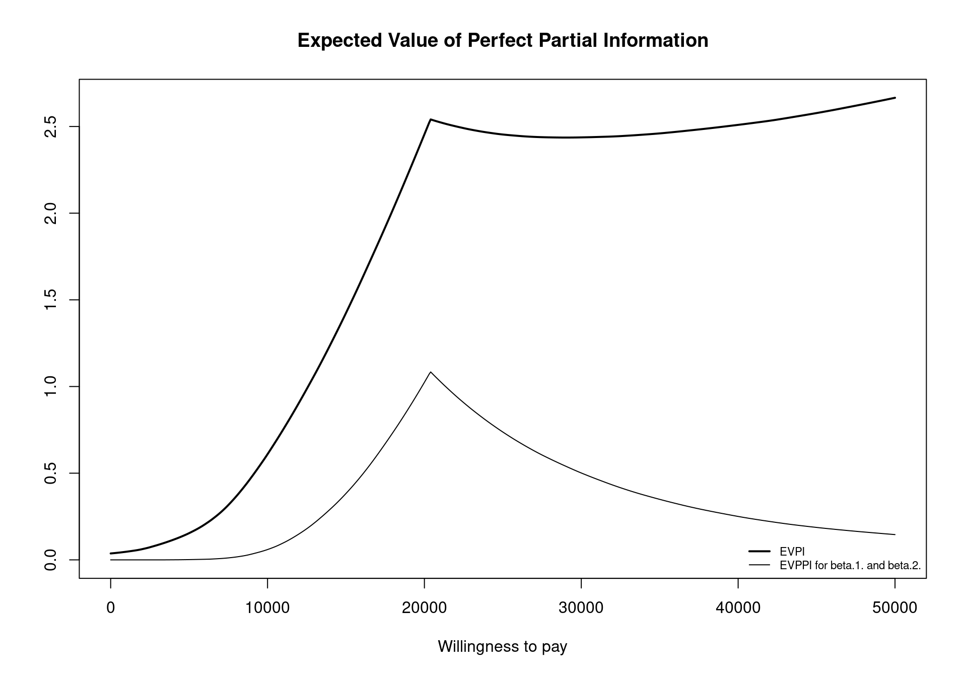
EVPPI <- evppi(m, c("beta.1.","beta.2."), inp$mat)As the evppi function can take some time to calculate the EVPPI, a read out of the progress is printed. The read out initially confirms the methods that are used to compute the conditional expectation. For computational simplicity, note that the conditional expectation for the costs and effects are estimated separately, which is why two methods are displayed, first the method for effects and then for costs. The most time consuming part of the EVPPI calculation is typically the Calculating fitted values for the GAM regression step, which is printed twice, once for effects and once for costs. Depending on the complexity of the problem, i.e., the number of parameters in \(\pmb\phi\) and the number of simulations used, this can take minutes.
It is possible to plot the evppi object using an S3 method for objects of the evppi class. This gives a graphic showing the EVPI and the EVPPI for all willingness to pay values included in the m$k vector (Figure 4.13), obtained by invoking the command plot(EVPPI) in the R terminal. In addition to this functionality, an evppi object contains objects that can be used for further analysis; these can be explored by typing
names(EVPPI)which returns the following output
 [1] "evppi"          "index"          "k"              "evi"
 [5] "parameters"     "time"           "method"         "fitted.costs"
 [9] "fitted.effects" "select"         "formula"        "pars"
[13] "res"
These elements can be extracted for individual analysis and relate to the following quantities.
evppi: a vector giving the EVPPI value for each value of the willingness to pay value inm$k.index: a vector detailing the column numbers for the parameters of interest.k: a vector of the willingness to pay values for which the EVPPI and the EVPI have been calculated.evi: a vector of the values for the EVPI for different values of the willingness to payparameters: a single character string detailing the parameters for which the EVPPI has been calculated. This character string is used to create the legend for the graphical output of theplotfunction.time: a list giving the computational time taken to calculate the different stages of the EVPPI estimation procedure.method: the calculation method used for the EVPPI. This will be alistobject (see Section 4.3.5.6).fitted.costs: this gives the estimated conditional expectations for costs, for the non-parametric regression methods presented in Section 4.3.3fitted.effects: as for costs, this gives the estimated conditional expectations for effects
The most important element of this object is the evppi vector giving the EVPPI values for the different willingness to pay values. In a standard analysis (using BCEA default settings) this whole vector can be quite unwieldy. However, the following code can be used to extract the EVPPI value for different willingness to pay thresholds, specifically in this case \(20,000\) monetary units.
EVPPI$evppi[EVPPI$k == 20000][1] 1.024234As previously discussed, the costs and effects are fitted separately in the evppi function, which contrasts with the theory presented in Section 4.3.3 and the original publication (Strong et al., 2014) Previously, the net benefit function \(U_t(\pmb\theta)\) was used as the response for the non-parametric regression. However, as the utility functions depend directly on the willingness to pay, this would implying calculating the EVPPI 501 times in a standard BCEA procedure. Therefore, to speed up computation the costs and effects are fitted separately and then combined for each willingness to pay threshold. Another computational saving is made by using incremental costs and effects as the response. This means that in a health economic model with \(T\) decision options, BCEA fits \(2(T-1)\) regression curves. In the process, bcea provides a read out of the progress and presents the computational time for each decision curve.
4.3.3.5 Example: Smoking (continued)
To demonstrate the evppi function for multi-decisions we use the smoking cessation example. Again, the simulations for each of the model parameters must be loaded into the R workspace. These simulations are contained in the rjags object smoking in the Smoking dataset — this was created by running the MTC model of Section 2.4.1 in JAGS. The following code is used to extract the parameter simulations from the rjags object:
inp <- createInputs(smoking_output)In the Smoking example, there are 20 parameters used to compute the costs and effects. To compute the EVPPI for the intervention specific relative effects for Self Help, Individual Counselling and Group Conselling, denoted \(d_1\), \(d_2\) and \(d_3\), respectively, we use the following code:
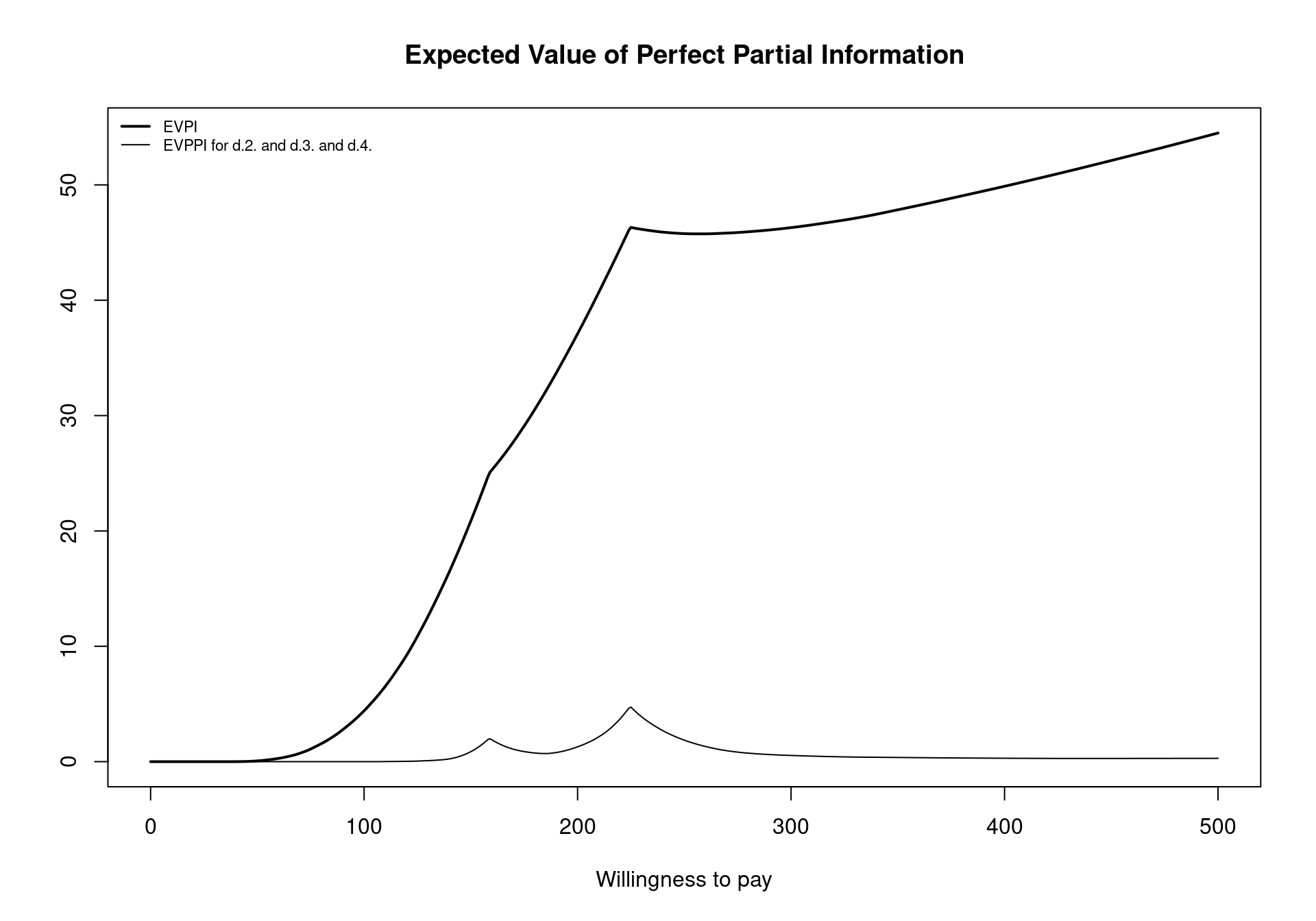
inp$parameters[c(1:3)][1] "d.2." "d.3." "d.4."EVPPI <- evppi(m, c(1:3), inp$mat)For the multi-decision example, we see that the read out from the evppi function is more long-winded as it includes three different calculations for the conditional expectation of the effects and three different calculations for the conditional expectation of the costs, as discussed in Section 4.3.3.4. With three parameters of interest, the GAM non-parametric regression method is slower than in the two parameter setting and the progress tracker is potentially useful, highlighting that the fitted values for GAM regression are found 6 separate times. Figure 4.14 shows the default EVPPI plot generated from this analysis using the code
plot(EVPPI, pos = "topleft")which positions the legend in the top-left corner of the plot using the pos argument. Again, notice that the two break-even points can be clearly seen for the EVPPI curve. Another key element to note is that the EVPPI is always dominated by the EVPI but the difference between the two curves does not remain constant for the different willingness to pay values.
smoking dataset for different willingness to pay values
An important consideration when computing EVPPI is that the non-parametric regression methods cannot be used when the parameters are constant values, particularly the GAM regression method. This is not critical as EVPPI for a constant parameter is 0 as the parameter is known with certainty. However, the evppi function does allow the inclusion of constant parameters, which can lead to errors. The createInputs function removes these columns from the BUGS or JAGS output so they cannot be considered for EVPPI analysis but if the user loads the parameters from another software, it is important to ensure that all parameters are subject to uncertainty.
4.3.4 Advanced Options
The evppi function can take extra arguments to allow users to manipulate the underlying estimation procedures. In general, these extra arguments fine tune the procedure to increase/decrease computational speed depending on the required accuracy of the estimate. As a general rule, the slower the estimation procedure, the more accurate the EVPPI estimation. Therefore, the user can prioritise either speed or accuracy. The default settings in BCEA are chosen as a trade off between these two considerations.
4.3.4.1 Selecting the number of PSA runs
The input N simply allows the user to control how many PSA runs are to be used to calculate the EVPPI. This is useful when a large number of PSA runs, say over \(5,000\), are available for analysis as the estimation methods for the EVPPI can be slow for large PSA samples and can sometimes crash due to the memory capabilities required for this methodology. It is advisable, therefore, to subset from this larger PSA sample and calculate the EVPPI using a smaller number of PSA simulations.
EVPPI <- evppi(m, c("beta.1.","beta.2."), inp$mat, N=250)In the above code, the EVPPI is computed with only 250 PSA simulations, rather than the 1000 PSA simulations available for the Vaccine example. In reality, it would be inadvisable to use 250 PSA simulations to compute EVPPI and 1000 would likely be the minimum number of simulations that should be used.
4.3.4.2 Outputting the residuals
As the estimation of the EVPPI is effectively the result of a complex statistical model it is important to check and evaluate the quality of this procedure. Thus, in line with standard statistical methodology, the function evppi allows the user to assess model fit. To do this, the option residuals must be set to TRUE or T (the default value). This argument should be changed to FALSE or F if the evppi objects become too large.
However, if the residuals argument is TRUE, then evppi outputs the estimated values for the function \(g_t(\pmb\phi)\), which can be used to check the modelling assumptions and thus give some confirmation that the EVPPI has been estimated correctly. Specifically, for the non-parametric regression methods, the residuals should look as if they were drawn from a Normal distribution — this is again in line with any linear or non-linear regression method. In addition to this, and more importantly, the residuals should have no underlying structure or graphical pattern.
BCEA contains a function diag.evppi that allows users to visually check these model assumptions. A typical call for this function is the following.
EVPPI <- evppi(m, c("beta.1.","beta.2."), inp$mat, residuals=TRUE)
diag.evppi(EVPPI, m, plot_type="residuals")
diag.evppi(EVPPI, m, plot_type="qqplot")
The function diag.evppi takes the output of the evppi function as its first argument so we start by esimating EVPPI within the BCEA package. In the code above, we emphasise that the residuals=TRUE is set (although this is the default). Critically, the diag.evppi function also requires the underlying bcea object m, which must relate to the same example for which EVPPI has been computed. If we set plot_type="residuals", then diag.evppi plots the residuals against the fitted values for both the costs and effects (see Figure 4.15). This plot should have no structure and be centered around 0. If the plot has clear structure or biased residuals, then the EVPPI estimate will be inaccurate.
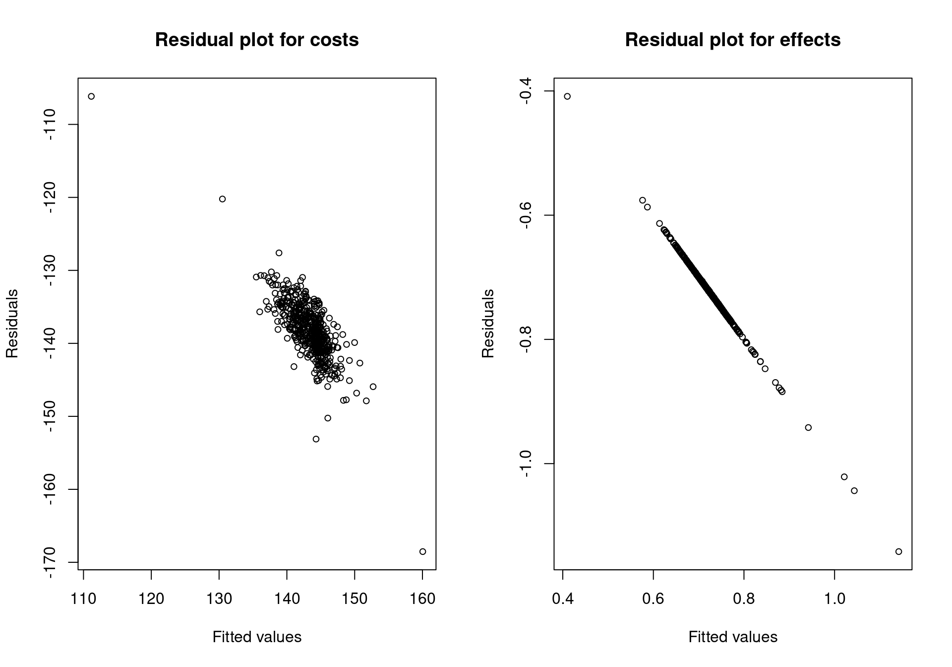
Setting plot_type="qqplot" shows a QQ-plot indicating whether the residuals are approximately distributed as a Normal random variable. This is a less important consideration but nevertheless can indicate if there are problems with the estimation procedure (see Figure 4.16).
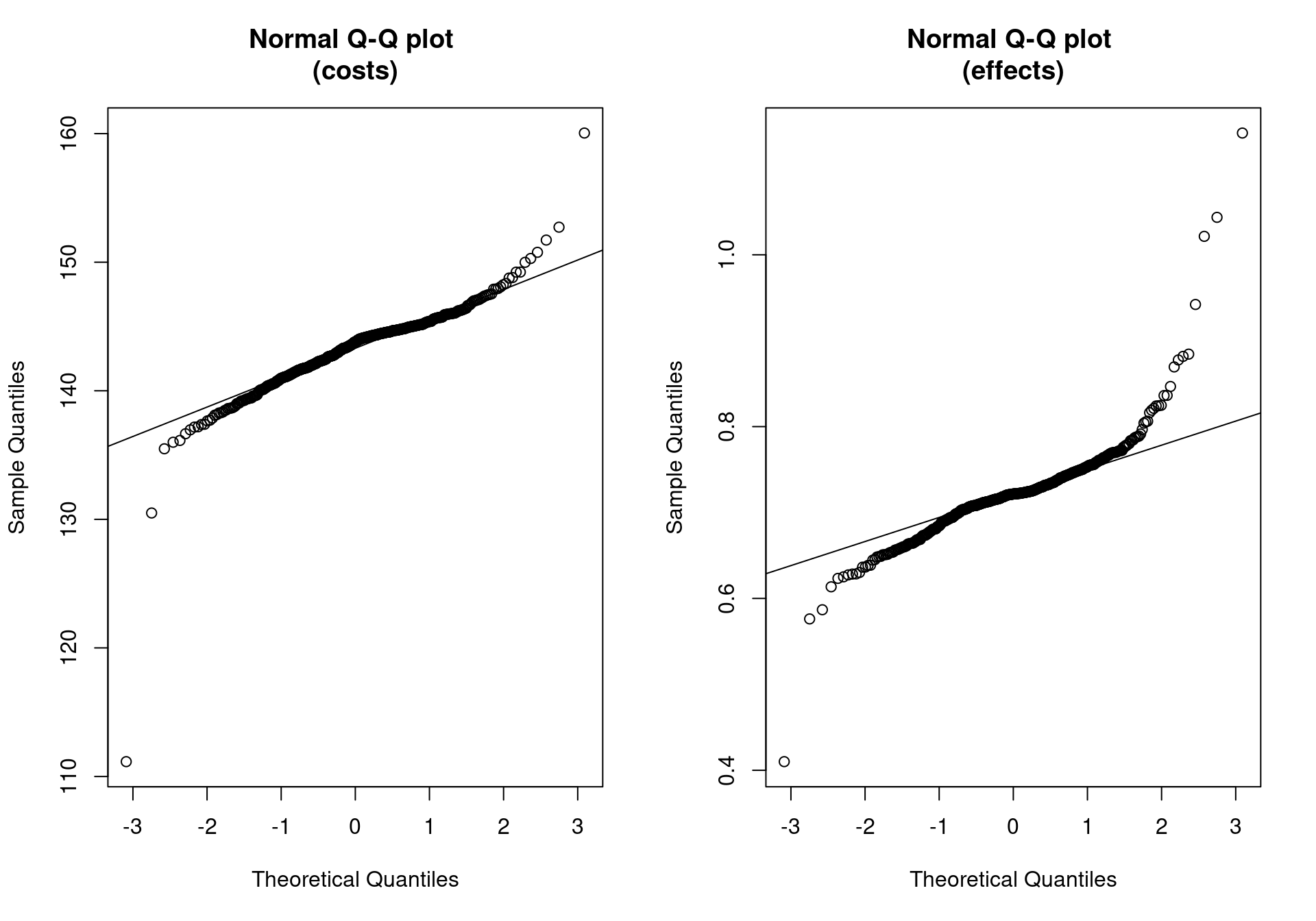
In a multi-decision problem, such as the Smoking example, \(g_t(\pmb\phi)\) must must be estimated separately for each comparison, for both costs and effects, as seen in Section 4.3.3.5. There are, therefore, a total of 6 functions to be estimated by regression methods. This is turn means there are 6 different regression fits that need to be checked. This can be done using the diag.evppi function using the additional argument int=k, where k is the column in the m$delta.e matrix for which we wish to asses the fit. For example, the call
diag.evppi(EVPPI, m, plot_type="residuals", int=2)would instruct BCEA to plot the regression fit for the second incremental costs and effects.
4.3.5 Technical options for controlling the EVPPI estimation procedure
This section relates to the more technical aspects for controlling the non-parametric estimation methods. This section is more advanced and assumes that the reader has read Section 4.3.3 and specifically Section 4.3.3.3. It is not necessary to use these additional fine tuning procedures to produce EVPPI estimates but in some more complicated health economic models it may be necessary to improve the EVPPI estimation accuracy using these more advanced manipulations.
4.3.5.1 EVPPI using non-default GAM regression
The default GAM regression method in the evppi function includes all interactions between parameters in \(\pmb\phi\), as discussed in Section 4.3.3.1. This gives maximum flexibility and therefore, in general more accuracy, inevitably at the cost of computational time. Additionally, when the number of hyperparameters needed to estimate the GAM approaches the number PSA simulations then the GAM overfits and the accuracy is compromised. For this reason, it is not recommended to use for the GAM for more than 4 parameters of interest (Heath et al., 2017) and this is the default in the evppi function.
However, to avoid overfitting for more parameters of interest, it possible to specify a different form of interaction structure among the parameters of interest. Firstly, to use the GAM method for more than 4 parameters of interest, the argument method="GAM" must be added to the evppi call. Secondly, the structure for the non-parametric regression is specified by adding the formula argument in the evppi call. The formula argument is passed directly to the gam function in the mgcv package. Therefore, a full explanation of the formula structure is given by executing ?gam or help(gam). In general, there are two key specifications that provide alternative spline formulations, s(), is a smooth function of 1 parameter, and te(), is a tensor product, which models interactions between several parameters. For example, lets assume \(\pmb\phi=(\beta_1,\beta_2,\lambda)\), we could specify formula="te(beta.1.,beta.2.) + s(lambda)"; this implies that \(g_t(\pmb\phi)\) is estimated by modelling interactions between \(\beta_1\) and \(\beta_2\), which could be correlated, and then modelling \(\lambda\) separately.
4.3.5.2 Controlling the INLA algorithm for multi-parameter EVPPI
An efficient alternative to GAM regression for multi-parameter EVPPI and the default for more than 4 parameters of interest is to use the INLA method, discussed in Section 4.3.3.3. Overall, the INLA algorithm is an approximate Gaussian Process regression method that uses numerical integration to approximate the hyperparameters of the GP. Specifically, the hyperparameters are estimated precisely at a small number of points throughout the support of these hyperparameters. The number of points, or more precisely the distance between these points must be chosen to control the accuracy and efficiency of the estimation procedure. By default, in the evppi function, this value is set to 0.00005 which is generally small enough to get accurate estimates for the EVPPI. However, in some settings this grid is not sufficiently fine, which break-downs the numerical approximation and the INLA algorithm crashes. If this does happen, then the distance between these points should be reduced by adding the h.value argument to the evppi call. Reducing the h.value will allow the INLA algorithm to estimate the EVPPI accurately.
4.3.5.3 Controlling the grid for the default INLA-SPDE Method
In addition to estimating the hyperparameters, the SPDE-INLA method adjusts a standard linear regression by approximating a “surface” that represents the impact of the GP covariance matrix on the conditional expectation. Similar to the hyperparameters, this surface is only estimated at certain points on a gird. This implies that the accuracy of the EVPPI and computational time depend directly on this grid. Therefore, there are several options in the evppi function that allow users to control the creation of the grid and through that control the estimation of the EVPPI.
To investigate the grid properties, the option plot=TRUE should be set in the call to evppi. This plots the grid for each function \(g_t(\pmb\phi)\) and also allows the user to save the grid during the estimation procedure. Figure 4.17 gives a good example of a grid used to approximate the EVPPI. The blue dots represent the PSA data whereas the vertices of the triangles are the points where the surface is estimated.
In principal, the grids should be broadly circular with no visual outliers — blue dots isolated from the other points by a blue boundary line. The inner section should have dense triangles with a boundary relatively tight to the blue data points. The outer section should be spaced away from the blue data points and can have larger triangles. Both these sections are encased by blue boundary lines.
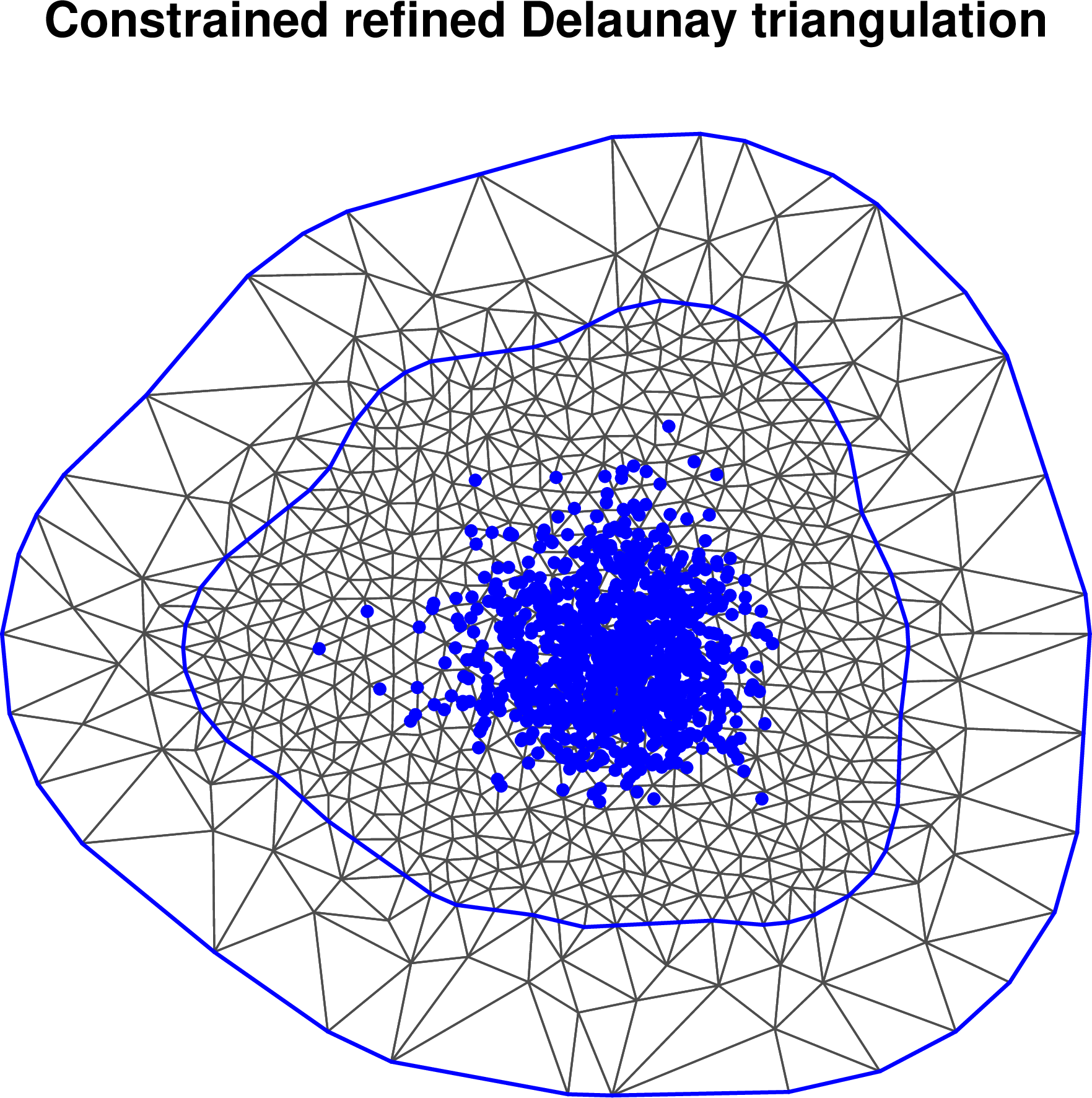
The closer these boundaries sit to the data the faster the computation as there are fewer grid points. However, the INLA method fixes the value of the surface at the outer boundary meaning that boundaries close to the data can skew the results. The inner (outer) boundary can be controlled using the argument convex.inner=a (convex.outer=a'), where a (a') is a negative value, typically between \(-0.2\) and \(-0.6\) for the inner and \(-0.5\) and \(-1\) for the outer boundary. Notice that the value a' should be more negative than a, as more negative values indicate that the boundary will be further from the points of interest.
Technically, these negative values define the minimum radius of the curvature of the boundary, defined as a fraction of the radius of the points. This means that, if convex.inner=-0.1 then the minimum curvature of the boundary has radius equal to one tenth of the radius of the points, giving a boundary that hugs the points of interest quite tightly. As this is decreased to more negative values, the boundary is constrained to be further from the points of interest. Incidentally, Figure 4.17 uses values of \(-0.3\) and \(-0.7\) respectively for the two boundaries.
The density of the points can also be controlled with the argument cutoff=b and max.edge=c, where b can typically be between 0.1 and 0.5 and c between 0.5 and 1.2. These values simply define the minimum and maximum (absolute) difference between the points in this grid. Small values increase the density and larger values decrease it, with the computation time varying inversely to the density of the grid points.
4.3.5.4 Modifying the linear predictor
As mentioned in Section 4.3.3.3, the basic idea of the INLA/SPDE procedure is to construct a model for \(g_t(\pmb\phi)\) which depends on a linear predictor \(H\pmb\beta\) and a “spatially structured” component \(\pmb\omega\) which allows us to account for correlation among the \(Q_\phi\) parameters in \(\pmb\phi\) and is based on 2 dimensional reduction of \(\pmb\phi\). Often, this 2-dimensional reduction is sufficient to capture all the information about \(\pmb\phi\) and successfully estimate the target function \(g_t(\pmb\phi)\) to produce an accurate estimation of the EVPPI. However, in some cases this reduction is not sufficient to capture all the information and bcea will give the user a warning:
Warning message:
In make.proj(parameter = parameter, inputs = inputs, x = x, k = k,  :
  The dimension of the sufficient reduction for the incremental effects,
  column 1, is 3. Dimensions greater than 2 imply that the EVPPI approximation
  using INLA may be inaccurate. Full residual checking using diag.evppi
  is required.
As is possible to see, the warning suggests residual checking as a means to identify any issues with the estimation. Additionally, it details which regression curve may be inaccurate, in this case the first incremental decision (int=1 for the diag.evppi command) and specifically for the incremental effects. Figure 4.18 shows the residual plot for the example above which is structured and therefore indicating some issues with the estimation procedure. As suggested in (Strong et al., 2014), it is important to note that while this error structure does show some issues with the estimation procedure these are not necessarily severe as the residuals are symmetric. This means that the mean \(g_t(\pmb\phi)\) is likely to be correctly estimated. As the EVPPI estimate is based on the estimate, it may still be accurate.
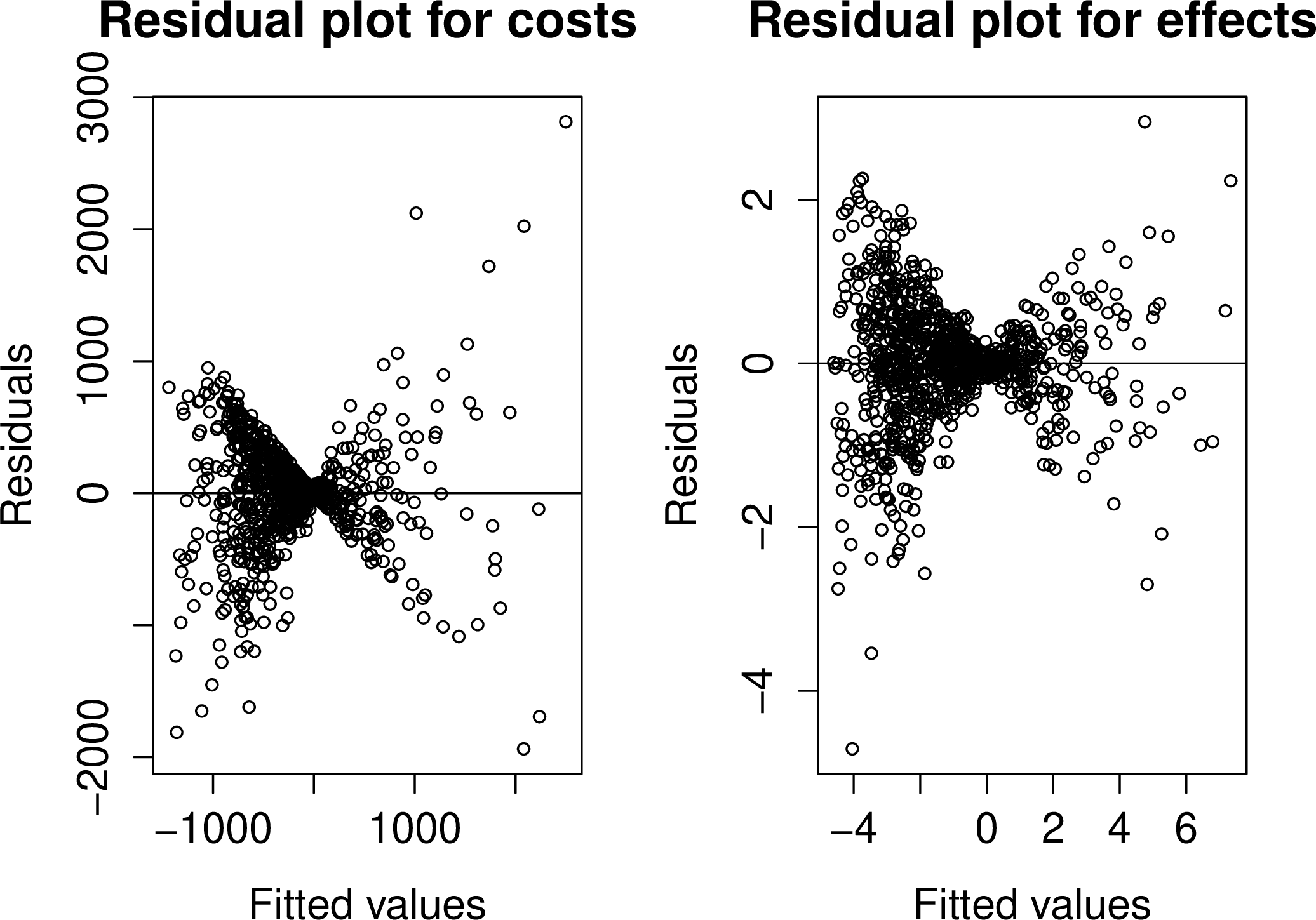
In general, the estimation of the conditional expectation can be improved by using the computational intensive standard GP regression procedure. However, as the issues may not be severe, the estimation can be improved with a smaller computational cost by modelling some level of interactions between the parameters in the linear predictor. These interactions can be added using the int.ord argument in the evppi function which can be given as a vector, \(e.g.\) int.ord=c(2,1). This formulation models second order interactions for the effects only, as the dimension reduction was unsuitable for the effects. This means, for example when \(\pmb\phi\) contains 3 elements, that the linear part of the model for the effects is changed to a non-linear structure \[
\beta_0 + \beta_{1}\phi_{1s} + \beta_{2}\phi_{2s} + \beta_{3}\phi_{3s} + \beta_{4}\phi_{1s}\phi_{2s} + \beta_{5}\phi_{1s}\phi_{3s} + \beta_{6}\phi_{2s}\phi_{3s}.
\] Clearly, this increases the number of regression parameters from \((Q_\phi+1)\) to \(\displaystyle Q_\phi + 1 + \left(\begin{array}{cc} Q_\phi \\ 2 \end{array}\right)\), giving an increase in computational time.
In a multi-decision case, it may be advisable to only use interactions for the curve where the issues occurred, in this case the first incremental effects, to avoid a large increase in computational time. This is achieved by using the list environment in R. The first element in the list is the interaction levels for the effects and the second is the interaction levels for the costs. So in this example, the following code would be used
interactions <- list(c(2,1,1), c(1,1,1))
EVPPI <- evppi(m, 1:3, inp$mat, int.ord=interactions)
to only use second order interactions for the first incremental effects.
Once the EVPPI has been fitted with interactions, we must reassess whether the EVPPI has been correctly estimated by inspecting the residuals. If this has not improved the fit significantly then either the interaction levels can be increased further or the non-default GP method should be used. However, both these strategies typically have a greater computational cost.
4.3.5.5 EVPPI using non-default GP regression
To use non-default GP regression for all regression fits, \(e.g.\) the costs and effects for all incremental decisions, the argument method="GP" must be included in the call to the evppi function. As discussed in Section 4.3.3.2, the hyperparameters for the non-default regression are estimated using numerical methods. This involves inverting a square matrix with the same number of rows and columns as the PSA simulations which is computationally expensive and is the main contributor to the computational cost of the hyperparameter estimation.
Therefore, the default for this method is to use 500 PSA simulations to calculate the hyperparameters. This can be increased, to improve accuracy, by using the argument n.sims=S, where S is larger than 500. The computational speed can also be increased by reducing this number, although clearly this affects accuracy. It is important to note that matrix inversion has a S\(^3\) cost, implying that doubling the PSA simulation size will increase the computational cost by 8. Additionally, the computational time is related to the number of parameters of interest in \(\pmb\phi\). Therefore, the computational time can increase to hours in complicated models with a large number of parameters of interest.
4.3.5.6 Mixed Strategy for EVPPI calculations
Throughout this section, we have repeatedly discussed the trade-off between computational speed and accuracy, which is relevant for all three non-parametric regression method for EVPPI calculation. In many settings, the computationally efficient GAM regression or fast GP regression based on INLA will be sufficient to estimate EVPPI accurately. However, inspection the residuals may indicate that these methods are not sufficient to estimate EVPPI accurately and additional computational time will be required to get more accurate results.
As the evppi procedure fits several regression curves to model all incremental costs and effects, it may be that some of the curves can be fitted with the faster procedures, while the more complex curves may require more computational time. To allow for this, the method argument can be given as a list object in R, similar to the int.ord argument for including interactions. Again, the first list element contains the methods that should be used for effects and the second list element contains the methods for the costs. The fast GP regression method is called "INLA". Therefore, using the same example as before, where the first incremental effects were poorly fitted, the following code would be used:
methods <- list(c("GP","INLA","INLA"), c("INLA","INLA","INLA"))
EVPPI <- evppi(m, 1:3, inp$mat, method=methods)
This strategy for EVPPI estimation demonstrates that while the default options for the evppi function have been chosen as a trade-off between computational time and accuracy, it is important to perform residual checking as part of an EVPPI procedure. It is not recommended to use the evppi function to perform entirely “black-box” estimation for the EVPPI as this can lead to misleading EVPPI estimates.
4.3.6 The Info-rank plot
Having accuracy computed EVPPI, we now discuss how these results can be displayed. As discussed previously, EVPPI can be used to design and prioritise future research but it can also be used as a tool to undertake sensitivity analysis and explore which parameters are driving uncertainty in the decision. The simplest method to achieve this is to used EVPPI to provide an “overall” assessment of the impact of each single parameter on the decision uncertainty. To this aim, BCEA has a specialised function info.rank which produces a plot of the univariate EVPPI for all the parameters of interest (as specified by the user). While this is not ideal, since correlation among parameters and model structure does have an impact on the joint value of the EVPPI (which is not a linear combination of the individual EVPPIs!), the Info-rank plot with all the model parameters ranked can be used as a sort of Tornado diagram, a tool often used in deterministic sensitivity analysis (Briggs et al., 2012).
For example, in the case of the Vaccine case study, we can obtain the Info-rank plot for all the underlying model parameters by using the following commands.
# Creates the object with the relevant inputs
inp <- createInputs(vaccine_mat)

# Makes the Info-Rank plot
info.rank(m, inp, graph = "ggplot2")
where m is the bcea object for the Vaccine example. The second argument of the info.rank function gives the parameters for which the relative importance should be calculated. In this setting inp, provided from the createInputs function, implies that the relative importance should be calculated for all parameters in the Vaccine model.
This creates the graph shown in Figure 4.19. The graph shows a set of bars quantifying the proportion of the total EVPI associated with each parameter. The larger the bar, the higher the impact of a given parameter on decision uncertainty. As mentioned above, care is needed in giving this graph an “absolute” interpretation — just because a parameter shows a relatively low position in the Info-rank plot, does not mean that there will be no value in investigating it in conjunction with other parameters.
However, it can be shown that the EVPPI of a set of parameters must be at least as big as the individual EVPPI values. Therefore, parameters with high individual EVPPI will always result in joint parameter subset with high value. But, nothing can be said about parameters with small individual EVPPI values especially in decision tree models which are typically multiplicative in the parameters. This means that learning the value of one of these parameters has little value as the other elements remain uncertain. However, learning all the parameters can greatly decrease decision uncertainty and therefore has large value to the decision maker. Nonetheless, the Info-rank plot gives an overview, which is perhaps useful (in conjunction with expert knowledge about the model parameters) to drive the selection of the subset \(\pmb\phi\) to be included in the full analysis of the EVPPI. In addition to the graph, the function info.rank automatically prints the complete ranking for the parameters selected. This is also stored in an element $rank.
The user can also select a specific value for the willingness to pay for which the Info-rank is computed and plotted by setting the argument wtp=value. The element value must be one of the elements of the willingness to pay grid, i.e. the values stored in m$k. The default value is determined as the break-even point from the bcea object containing the economic evaluation. It is important to note that the ranking can change substantially as a function of the willingness to pay.
Additional options include graphical parameters that the user can specify. For example, the argument xlim specifies the limits of the \(x-\)axis; the argument ca determines the font size for the axis label (with default value set at 0.7 of the full size); cn indicates the font size for the vector of parameter names (again with default at 0.7 of the full size); mai specifies the margins of the graph (default = c(1.36,1.5,1,1)); and finally rel is a logical argument that specifies whether the ratio of EVPPI to EVPI (which can be obtained by default as rel=TRUE) or the absolute value of the EVPPI (rel=FALSE) should be used for the analysis.
4.3.7 Expected Value of Sample Information
Once EVPPI has identified parameters that have high value and may be prioritised for future research, the Expected Value of Sample Information (EVSI — Ades et al., 2004) can be computed to understand the value that could be obtained through a specific study with a known design. Strictly speaking, EVSI analyses are required to understand the true value of future research and perform research prioritisation. However, the complexity of EVSI analyses exceeds the complexity of EVPPI analysis as the study in question must be designed and data simulated from that study design (Heath et al., 2022). As such, it is beyond to scope of this book as calculation methods to compute EVSI are not implemented within BCEA. However, the recently developed voi package has extended the methods available in BCEA to include EVSI calculation methods. A complete presentation of the voi package and the calculation methods for EVSI are available in Heath and Kunst (2024).
4.4 PSA applied to model assumptions and structural uncertainty
This section is concerned with testing the sensitivity of the cost-effectiveness analysis to the underlying model and health economic modelling assumptions.
4.4.1 Mixed strategy
In the previous chapters we have explored the analysis of cost-effectiveness assuming that technologies and interventions would be used in total isolation, i.e., they would completely displace each other when chosen. In reality this happens rarely, as new interventions are not completely implemented for all patients in a certain indication. In general, the previous strategies usually maintain a share of the market over time. This is due to a number of factors, for example resistance to the novel intervention or preference of use of different technologies in different patients.
When the market shares of the other available technologies cannot be set to zero, the expected utility in the overall population can be computed as a mixture: \[ \bar{\mathcal{U}}=\sum_{t=1}^T q_t \mathcal{U}^t = q_1 \mathcal{U}^1 + q_2 \mathcal{U}^2 + \cdots + q_T \mathcal{U}^T \] with \(q_t\geq 0 \; \forall t \in \{1,\ldots,T\}\) and \(\sum_t q_t = 1\). For each intervention \(t\), the quantity \(q_t\) represents its market share and \(\mathcal{U}^t\) its expected utilities. The resulting quantity \(\bar{\mathcal{U}}\) can be easily compared with the “optimal” expected utility \(\mathcal{U}^*\) to evaluate the potential losses induced by the different market composition. In other terms, the expected utility for the chosen market scenario is the weighted average of the expected utility of all treatment options \(t\) with the respective market share \(q_t\) as weights.
4.4.1.1 Example: Smoking cessation (continued)
To evaluate the uncertainty surrounding the decision under a mixed-strategy assumption using the EVPI, the mixedAn function is provided in BCEA, which requires the bcea object, m, and the shares for each intervention. In general, it is useful to create an object containing the weights associated to each treatment strategy which we call mkt.shares. Its elements should be values between zero and one, and sum to one. The length of the vector needs to be equal to the number of interventions defined in the bcea object, i.e. equal to m$n.comparators, equal to four in the smoking cessation example. It is important to note that this function allows any values for the market shares (including negative shares and sum not equal to one), therefore the user needs to be careful when specifying them.
Let us assume that the market shares are driven by the willingness of the individuals to start therapies. In a possible scenario, the majority of the patients prefer quitting smoking without any help, and the other patients are less willing to undergo therapies as they become more costly. We can therefore imagine in this scenario that 40% of the individuals are in the no treatment group, 30% in the self-help group, and only 20% and 10% seek individual and group counselling respectively. The market shares vector are then defined as:
mkt.shares <- c(0.4, 0.3, 0.2, 0.1)To produce the results for the mixed analysis, it is necessary to execute the mixedAn function, to create an object ma or the class mixedAn.
mixedAn(m) <- mkt.sharesThe resulting m object can be used in two ways:
- To extract the point estimate of the loss in EVPI for a given willingness to pay value, by comparing the “optimal” situation in which the most cost-effective comparator \(t\) is adopted (such that the associated market shares \(q_t\) are equal to one);
- To produce a graphical analysis of the behaviour of the EVPI over a range of willingness to pay values for the mixed-strategy and “optimal” choice.
The first item can be obtained using the summary function. Since this is an S3 function for the objects of class mixedAn, the relative help page can be found by executing the ?summary.mixedAn function from the R console. For example the point estimate for the loss in EVPI for a willingness to pay of 250 per QALY gained can be obtained with:
summary(m, wtp=250)
Analysis of mixed strategy for willingness to pay parameter k = 250

Reference intervention: Group counselling (2.50% market share)
Comparator intervention(s): No intervention (10.00% market share)
                          : Self-help (7.50% market share)
                          : Individual counselling (5.00% market share)

Loss in the expected value of information = 110.08
The two EVPI curves, for the optimal and mixed-treatment scenarios together, can be plotted using the evi.plot function. Both the base graphics and ggplot2 versions of the plot are available, and can be selected by specifying the argument graph="base" (or "b" for short, the default) or graph="ggplot2" (or "g" for short). The function accept other arguments analogously to the previously presented functions to tweak the appearance of the graph in addition to the choice of the plotting library to be used (the help page can be opened by running ?evi.plot.mixedAn in the R console). The y-axis limits can be selected by passing a two-element vector to the argument y.limits (defaults to NULL), while the legend position can be chosen using pos, consistent to other functions such as ceplane.plot. The output of the function for the code shown below is presented in Figure 4.20.
evi.plot(m, graph="g", pos="b")Figure 4.20 shows the behaviour of the EVPI over willingness to pay values ranging from \(0\) to \(500\). The EVPI for the mixed strategy is greater than the optimal strategy scenario, in which the whole of the market share is allocated to the intervention with the highest utility at any given willingness to pay value. The gap between the two curves is wider for the two extreme points of the chosen interval of WTP values, while they are relatively close in the interval between \(150\) and \(250\) per life years gained. This is because in this interval the decision uncertainty is highest, which decreases the opportunity loss differential between the two scenarios. Clearly, when the optimal strategy is uncertain then all strategies are similar and therefore using a mixed strategy is actually close to the optimal strategy.
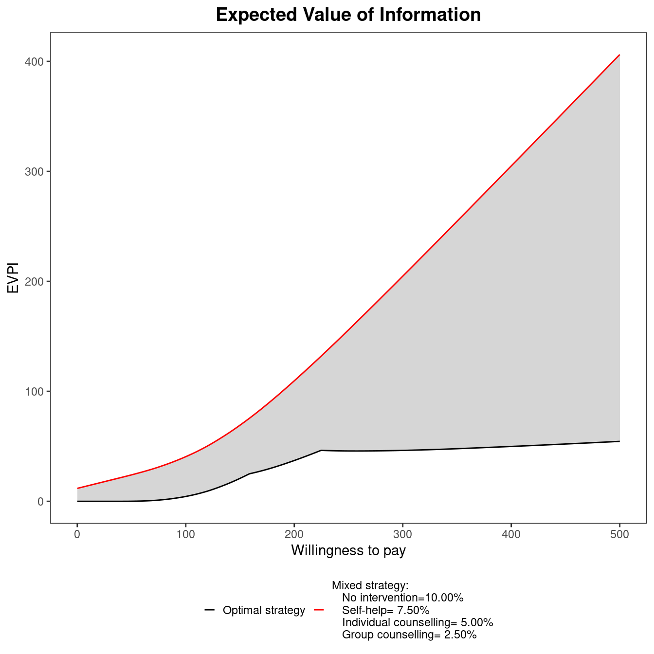
4.4.2 Including risk-aversion in the utility function
In all the analyses presented so far, the utility for the decision maker has always been assumed to be described by the monetary net benefit (see Section 1.3). This assumption imposes a form of risk neutrality on the decision maker, which might not be always reasonable (Baio, 2012). A scenario considering risk aversion explicitly, with different risk aversion profiles, can be implemented by extending the form of the utility function (Baio and Dawid, 2011). One of the possible ways to include the risk aversion in the decision problem is to re-define the utility function Equation 1.5 as: \[ u(b,r) = \frac{1}{r}\left[1-\text{exp}(-rb) \right] \] where the parameter \(r>0\) represents the risk aversion attributed to the decision maker. The higher the value of \(r\), the more risk-averse the decision maker is considered to be, where \(b:=ke-c\) is the monetary net benefit.1
It is not usually possible to make the degree of risk aversion explicit, as it is unlikely to be known. Therefore an analysis using different risk aversion scenarios can be carried out to analyse the decision making process as a function of \(r\).
The CEriskav function provided in BCEA can be used to perform health economic analysis in the presence of risk aversion. In a similar manner to the mixed strategy analysis presented in Section 4.4.1, a new object is created after the user specifies the risk aversion parameter \(r\). This can be a single positive number or a vector of possible values denoting the risk aversion profile of the decision maker. A vector r can be defined and fed into the function together with the bcea object.
4.4.2.1 Example: Vaccine (continued)
To perform the analysis with risk aversion we will use the Vaccine example. We will assume that the object m of class bcea, produced by the initial call to the function bcea and containing the results of the base case analysis, is available in the current workspace. A vector r containing the risk aversion parameters to be used in the scenarios. To assess the robustness of the results to variations in risk aversion, we input different values in a vector, r.
r <- c(1e-10, 0.005, 0.020, 0.035)The first element is taken to be sufficiently close to zero to be interpreted by bcea as a scenario with no risk aversion, marked as \(r \to 0\) on the graphic, Figure 4.21. Once the \(r\) vector is defined, the risk aversion analysis can be run by using the function CEriskav. This will extend the \(m\) object and additionally assign the class CEriskav:
CEriskav(m) <- rThe objects of class CEriskav can be used to produce the expected incremental benefit and expected value of perfect information plots in BCEA. To do so it is sufficient to call the plot function with an object of class CEriskav as argument. This will produce the output displayed in Figure 4.21.
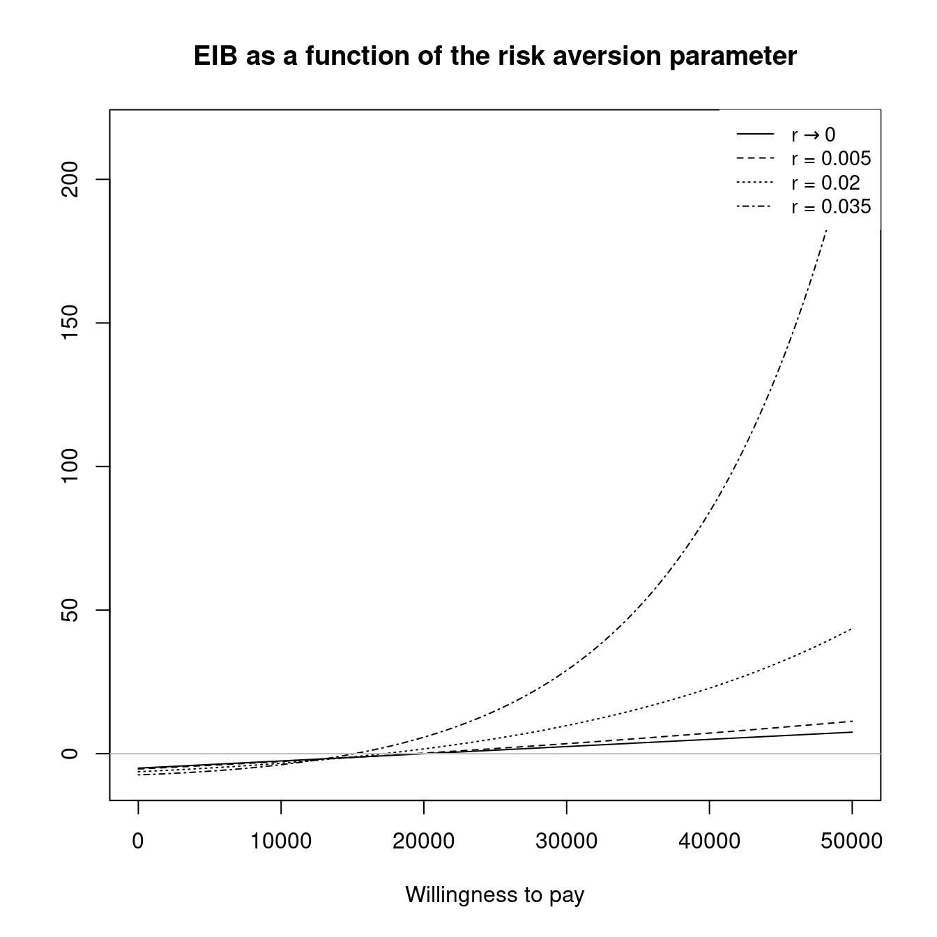
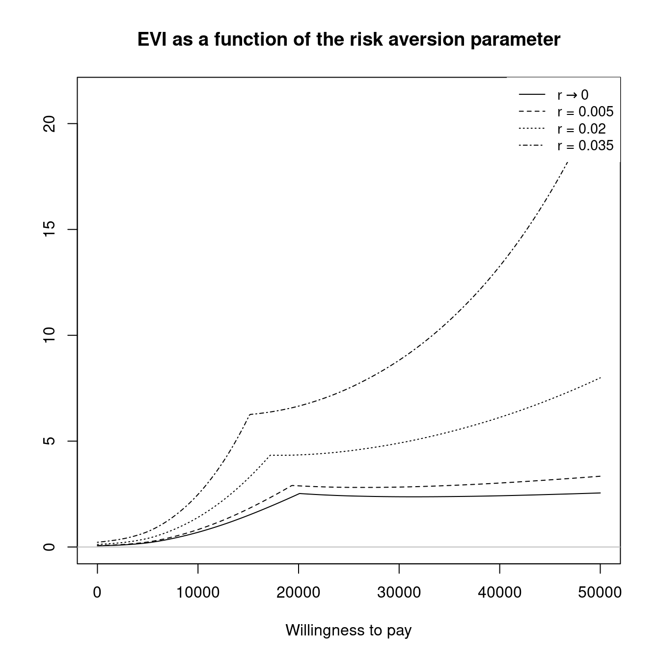
Calling the plot function with a CEriskav object (i.e. the plot.CEriskav function) will produce the two graphs in two separate graphical windows by default. This creates a new graphical device for the second plot (the EVPI). This behaviour can be modified by passing additional arguments to the plotting function. If the argument plot="ask" is added, the "ask" option in the graphical parameters list "par" will be temporarily be set to TRUE. In this way the second plot will be displayed in the active device, after the application receives, either the Return key, in an interactive R session, or readline() in non-interactive sessions.
Objects of class CEriskav contain several subsettable named elements:
Ur: a four-dimensional numeric matrix containing the utility value for each simulation, willingness to pay value (WTP) contained in the approximation grid vectork, intervention and risk aversion parameter included in the vectorr;Urstar: a three-dimensional numeric matrix containing the highest utility value among the comparators for each simulation, willingness to pay value in the approximation grid and risk aversion parameter;IBr: the incremental benefit matrices for all risk aversion scenarios, built as three-dimensional matrices over the simulation, WTP values and values defined inr;eibr: the EIB for each pair of WTP and risk aversion values, i.e. the average ofIBrover the simulations;vir: the value of information, in a multi-dimensional matrix with the same structure asIBr;evir: the expected value of information obtained averagingvirover the simulations;R: the number of risk aversion scenarios assessed;r: the input vector \(r\), containing the risk aversion parameters passed to theCEriskavfunction;k: the grid approximation of the interval of willingness to pay values taken from thebceaobject given as argument toCEriskav, in this casem.
4.4.3 Probabilistic sensitivity analysis to structural uncertainty
All the sensitivity analyses presented so far are based on the premise that the only way in which uncertainty affects the results of the economic evaluation is either through sampling variability for the observed data or epistemic uncertainty in the parameters that populate the model. In other words, the economic assessment is performed conditionally on the model selected to describe the underlying phenomenon.
However, almost invariably the model structure, i.e. the set of assumptions and alleged relationships among the quantities involved, is an approximation to a complex reality. As Box and Draper state; “all models are wrong, but some are useful” (Box and Draper, 1987).
From a hard-core Bayesian perspective, the ideal solution would be to extend the modelling to include a prior distribution over a set of \(H\) finite, mutually exclusive and exhaustive potential model structures \(\mathcal{M}=(\mathcal{M}_1,\mathcal{M}_2,\ldots,\mathcal{M}_H)\). In principle, these may be characterised by some common features (i.e. some Markov model to represent the natural history of a disease) and each could have slightly different assumptions; for example, \(\mathcal{M}_1\) may assume a logNormal distribution for some relevant cost, while \(\mathcal{M}_2\) may assume a Gamma.
In this case, the data would update all the prior distributions (over the parameters within each model and over the distribution of models) so as to determine a posterior probability that each of the \(\mathcal{M}_h\) is the “best” model (\(i.e.\) the one that is most supported by the data). It would be possible then to either discard the options with too small posterior probabilities or even build some form of model average, where the weights associated with each structure are these posterior probabilities. Leaving aside the technical difficulties with this strategy, the main problem is the underlying assumption that we are able to fully specify all the possible alternative models. This is rarely possible in practical scenarios.
One possible way to overcome this issue is to aim for a less ambitious objective — the basic idea is to formalise a relatively small set of possible models and compare them in terms of their out-of-sample predictions. This quantifies how well the predictive distribution for a given model would fit a replicated dataset based on the observed data. Notice that, especially in health economic evaluations, the possible models considered are merely a (rough) approximation to the complex phenomenon under study, so there is unlikely to be a guarantee that any of these models should be the “true” one.
Under this strategy, it is therefore necessary to determine a measure of goodness of fit that can be associated with each of the models being compared. Within the Bayesian framework, one convenient choice is to use the Deviance Information Criterion (DIC) (Spiegelhalter et al., 2004). A technical discussion of this quantity and its limitations is beyond the objectives of this book — for a brief discussion see (Baio, 2012). Nevertheless, the intuition behind it is that it represents a measure of model fit based on (a function of) the likelihood \(D(\theta) = -2\log p(y\mid\theta)\) and a term \(p_D\), which is used to penalise model complexity. The reason for the inclusion of the penalty is that models containing too many parameters will tend to overfit the observed data, i.e. do particularly well in terms of explaining the realised dataset, but are likely to perform poorly on other occurrences of similar data.
From the technical point of view, it is fairly easy to compute the DIC as a by-product of the MCMC procedure. Structural PSA can be then performed by using the following steps.
- Define a (relatively small) set of possible models \(\mathcal{M} = (\mathcal{M}_1,\mathcal{M}_2,\ldots,\mathcal{M}_H)\). These may differ in terms of distributional assumptions, but may also contain slightly different features.
- Fit all the models and for each \(h=1,\ldots,H\), compute DIC\(_h\). This usually has no extra computational cost;
- Derive a set of weights to be associated with each of the models. One possible solution discussed in (Baio, 2012) is to use \[ w_h = \frac{\exp(-0.5\Delta\mbox{DIC}_h)}{\displaystyle\sum_{h=1}^H \exp(-0.5\Delta\mbox{DIC}_h)}, \tag{4.7}\] where \(\Delta\mbox{DIC}_h = \mid \min_h(\mbox{DIC}_h) - \mbox{DIC}_h\mid\);
- Use the weights \(w_h\) to compute an average model \(\mathcal{M}^*\).
4.4.3.1 Example: Chemotherapy
To consider this strategy, we consider a model discussed in Baio (2012) used to evaluate a new chemotherapy drug (\(t=2\)) against the standard of care \((t=1)\). A graphical representation of the modelling structure is shown in Figure 4.22: in each treatment option, patients may experience blood-related side effects (with a probability \(\pi_t\)) or can have an successful treatment, where no side effects occur, with probability \((1-\pi_t)\). In the latter case, the measure of effectiveness \(e_t\) is set to 1, while the only cost accrued is the acquisition of the drug \(c_t^{drug}\), which varies in the two arms. In the presence of side effects, patients may require ambulatory care (with probability \(\gamma\), which we assume is independent on the treatment assigned); this is coded as a non-effective treatment and thus \(e_t=0\); the patients in this branch of the decision tree will accrue costs \(c_t^{drug} + c_t^{amb}\). Similarly, the patients who experience the worst side effects will go into hospital, which we simplistically assume happens with probability \((1-\gamma)\) and will accrue costs \(c_t^{drug} + c_t^{hosp}\).
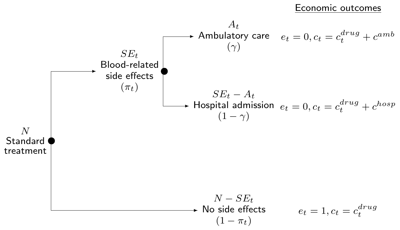
The new drug is supposed to produce a reduction in the chance of side effects, so that we can model \(\pi_1 = \rho\pi_0\), where \(\pi_0\) is a baseline value, which is associated with the standard of care, and \(\rho\) is the reduction factor.
We can express the assumptions in terms of a fairly simple model, where the number of patients experiencing side effects is \(SE_t\sim\mbox{Binomial}(\pi_t,n_t)\); conditionally on the realisation of this event, the number of patients requiring ambulatory care is \(A_t\sim\mbox{Binomial}(\gamma,SE_t)\). We also assume a vague prior on the probability of side effects under the standard of care and on the probability of ambulatory care, \(e.g.\) \(\pi_0,\gamma \stackrel{iid}{\sim}\mbox{Beta}(1,1)\). A clinical trial may be conducted to investigate the new drug and we assume to have observed that \(n_0=111\), \(SE_0=27\), \(A_0=17\), \(n_1=103\), \(SE_1=18\) and \(A_1=14\). Notice that the trial data are about a sample of patients \((n_0,n_1)\) in the two arms, while we are interested in extrapolating the model to the target population, made by \(N\) individuals (as shown in Figure 4.22).
We also assume that some information, \(e.g.\) from registries, is present to inform the prior distribution for the cost of ambulatory and hospital care and that this can be encoded in the following form: \(c^{amb} \sim \mbox{logNormal}(4.77,0.17)\) and \(c^{hosp} \sim \mbox{logNormal}(8.60,0.17)\). These imply that we are expecting them to realistically vary in the intervals £\((85\); £\(165)\) and £\((3813\); £\(7738)\), respectively. Moreover, we know that the drugs have fixed costs \(c_0^{drug}=110\) and \(c_1^{drug}=520\).
Arguably, the crucial parameter in this model is the reduction in the probability of side effects \(\rho\). We assume that only limited evidence is available on the actual effectiveness for \(t=1\) and thus consider two somewhat contrasting scenarios. In the first one, we model \(\rho \sim \mbox{Normal}(0.8,0.2)\), to express the belief that the new chemotherapy is on average 20% more effective than the standard of care, with some relatively limited variability around this estimate. The second scenario assumes a “sceptical” view and models \(\rho \sim \mbox{Normal}(1,0.2)\). This implies that on average the new chemotherapy is no better than the status quo, while allowing for uncertainty in this assessment. Figure 4.23 shows a graphical representation of these two prior distributions — panel (a) shows the “enthusiastic” prior, while panel (b) depicts the “sceptical” prior.
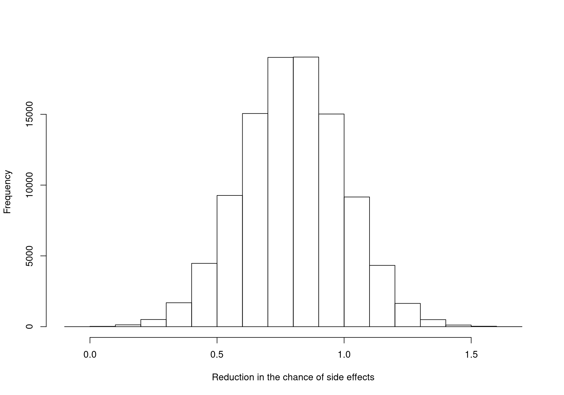
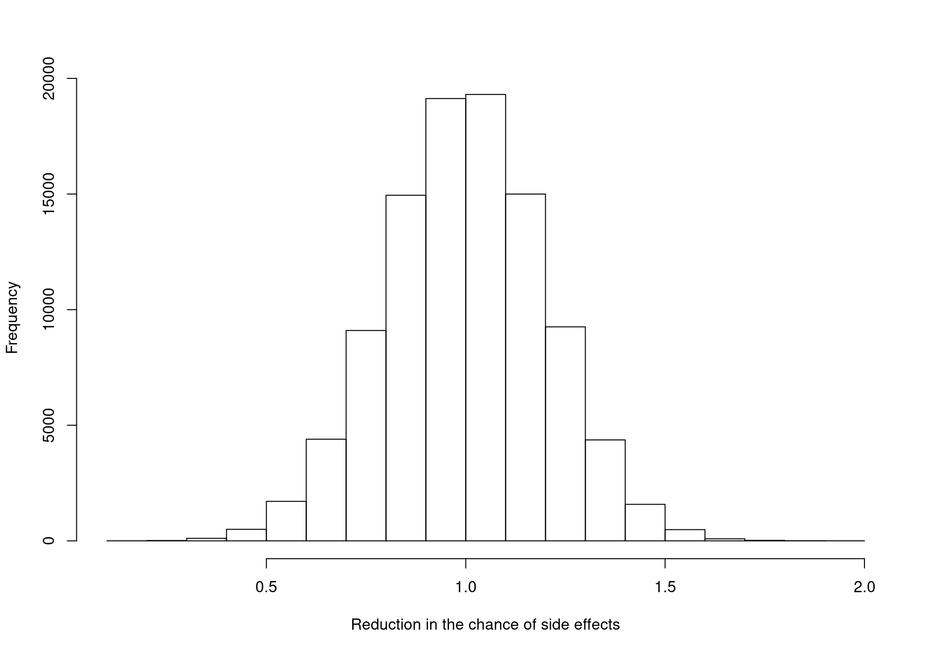
The model assumptions can be encoded in the following BUGS/JAGS code (notice that again we define the two treatment arms as \(t=1,2\) for the standard of care and the new drug, respectively).
model {
    # Observed data
    for (t in 1:2) {
        SE[t] ~ dbin(pi[t],n[t])
        A[t] ~ dbin(gamma,SE[t])
    }

    # Priors for clinical parameters
    pi[1] ~ dbeta(1,1)
    rho ~ dnorm(m.rho, tau.rho)
    tau.rho <- pow(sigma.rho,2)
    pi[2] <- rho * pi[1]
    gamma ~ dbeta(1, 1)

    # Priors for the costs
    c.amb ~ dlnorm(4.77,0.17)
    c.hosp ~ dlnorm(8.60,0.18)

    # Prediction for the whole target population
    for (t in 1:2) {
        # Estimated patients with side effects & ambulatory care
        SE.pred[t] ~ dbin(pi[t],N)
        A.pred[t] ~ dbin(gamma,SE.pred[t])

        # Defines economic output
        mu.e[t] <- 1-pi[t]
        mu.c[t] <- c.drug[t]*(1-pi[t]+pi[t]*(1-gamma)+pi[t]*gamma)+
            pi[t]*(1-gamma)*c.hosp+pi[t]*gamma*c.amb
    }
}
We allow for the two different formulations of the model by passing two sets of values for the parameter m.rho (set to 0.8 and 1 in the two cases). In this particular case, we are assuming that the standard deviation sigma.rho does not vary in the two scenarios, but of course this assumption could (and perhaps should) be relaxed.
The two models can be run using the R2jags package and the results may be stored in R objects, say chemo_enth and chemo_scep, both in the class rjags and containing the results of the MCMC simulations2.
# Loads the model results from the BCEA website
library(BCEA)
load("data/chemo_PSA.Rdata")

# Stores the two model files in the object 'models'
models <- list(chemo_enth, chemo_scep)

# Defines effects & costs as lists
e <- list(chemo_enth$sims.list$mu.e, chemo_scep$sims.list$mu.e)
c <- list(chemo_enth$sims.list$mu.c, chemo_scep$sims.list$mu.c)

# Performs structural PSA using BCEA
ints <- c("Standard of care", "New chemotherapy")
m_enth <- bcea(e[[1]], c[[1]], ref=2, interventions=ints)
m_scep <- bcea(e[[2]], c[[2]], ref=2, interventions=ints)
m_avg <- struct.psa(models, e, c, ref=2, interventions=ints)
In the code above, first we upload the results from the two models which are stored in the remote server. Then we create an R list in which we include the two objects chemo_enth and chemo_scep. The simulated values for the economic output defined in the model code in the nodes mu.e and mu.c can be accessed using the list format, by using the sims.list element inside the two model objects. For simplicity, we save these in two new objects e and c — notice that these will be lists containing two elements each, one from the “enthusiastic” and one from the “sceptical” model.
With these variables we can now perform basic analysis for each of the two models; we do this by calling the function bcea and applying it to the relevant elements of e and c — the notation e[[1]] instructs R to consider the first element of the object e (\(i.e.\) the simulated values for the effectiveness variable for the “enthusiastic” model, which is the first to be included in the object e). Similarly, e[[2]] indicates the second element (associated with the “sceptical” model).
Finally, we can use the bcea function struct.psa and perform the structural PSA. This function takes the list of models and the two lists including the measures of effectiveness and costs as arguments. The other (optional) arguments have the same format as the standard call to the function bcea and allow the user to specify the reference intervention and a vector of labels.
The resulting object m_avg is a list, whose element can be explored by typing the following commands
# Lists the elements of the object m_avg
names(m_avg)
[1] "n_sim" "n_comparators" "n_comparisons" "delta_e"
[5] "delta_c" "ICER" "Kmax" "k"
[9] "ceac" "ib" "eib" "kstar"
[13] "best" "U" "vi" "Ustar"
[17] "ol" "evi" "ref" "comp"
[21] "step" "interventions" "e" "c"
[25] "w" "DIC" # Shows the weights given to each model
m_avg$w[1] 0.4347864 0.5652136# Shows the DIC associated with each model
m_avg$DIC[1] 23.34652 22.82182The element m_avg$w is the vector of the weights associated with each of the models, as defined in Equation 4.7. In this case, the two models show relatively similar level of fit in terms of the DIC and thus the two values \(w_1\) and \(w_2\) are relatively close to 0.5, although, in light of the observed data, the sceptical model seems to be preferred and thus associated with a slightly higher weight. In other words, the evidence is perhaps not strong enough to support the bold claim that the new drug is substantially more effective than the standard of care.
This is consistent with the analysis of the two DICs, which can be explored from the element m_avg$DIC; the values are fairly close, although the one for the “sceptical” model is lower, indicating a (slightly) better fit to the observed data.
The remaining elements stored in the object m_avg are from an object in the class bcea. Thus, we can apply any BCEA command to the object m_avg for example we could type plot(m_avg), or contour2(m_avg). Figure 4.24 shows a comparison of the results from the three models. Panels (a) and (b) present the contour plot for the two original models, while panel (c) depicts the results of the economic evaluation for the model average. In the latter, the value of the ICER is some sort of compromise between the values of the two original models, while the variability of the posterior distribution \(p(\Delta_e, \Delta_c)\) appears to be reduced.
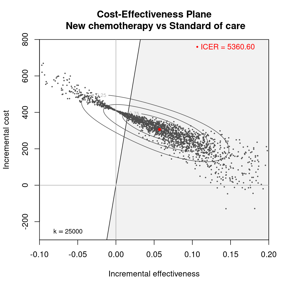
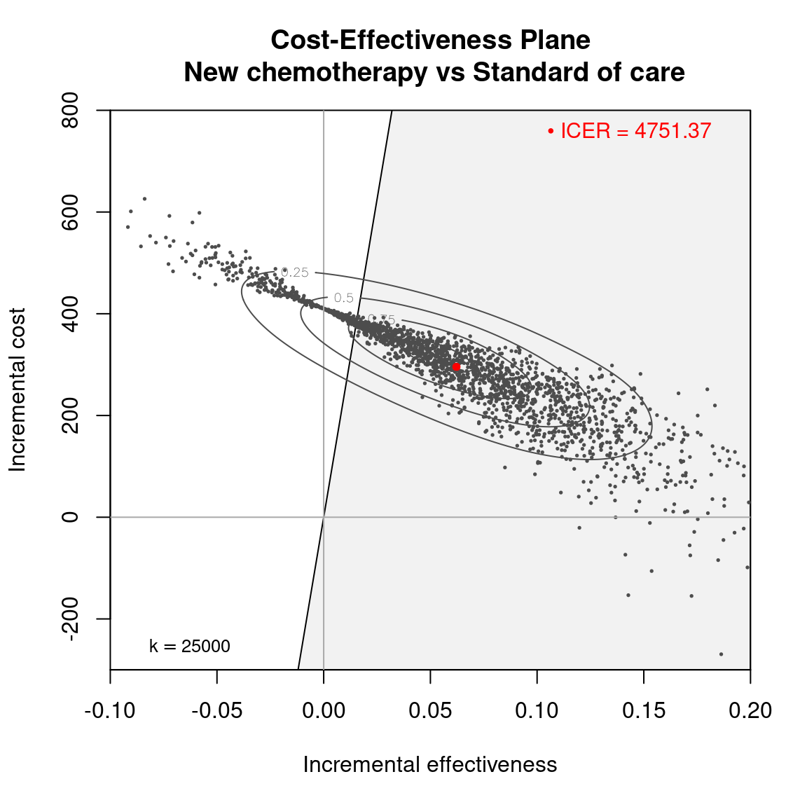
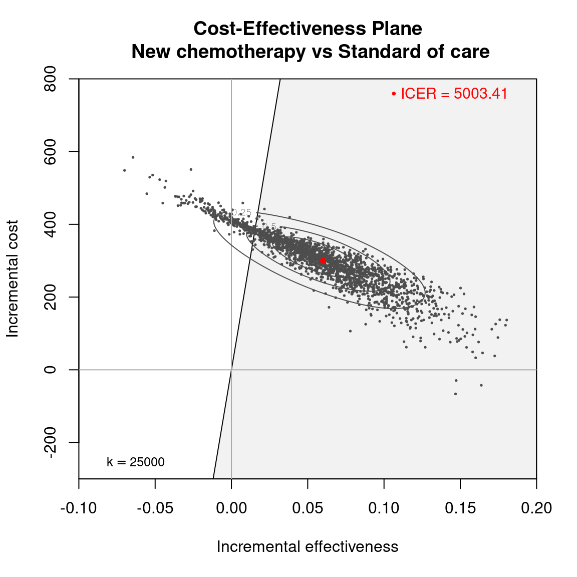
Figure 4.25 shows a comparison of the three models in terms of the CEAC in panel (a) and the of the EVPI in panel (b). Uncertainty in the model average has a lower impact on the decision-making process, as the CEAC is higher and the EVPI is lower for the model average. This is true for all the selected values of the willingness to pay, \(k\).
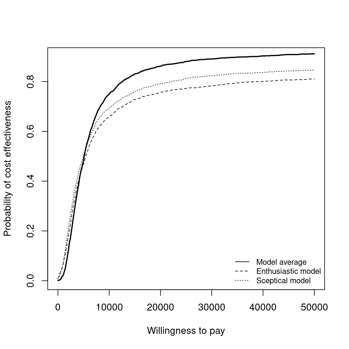
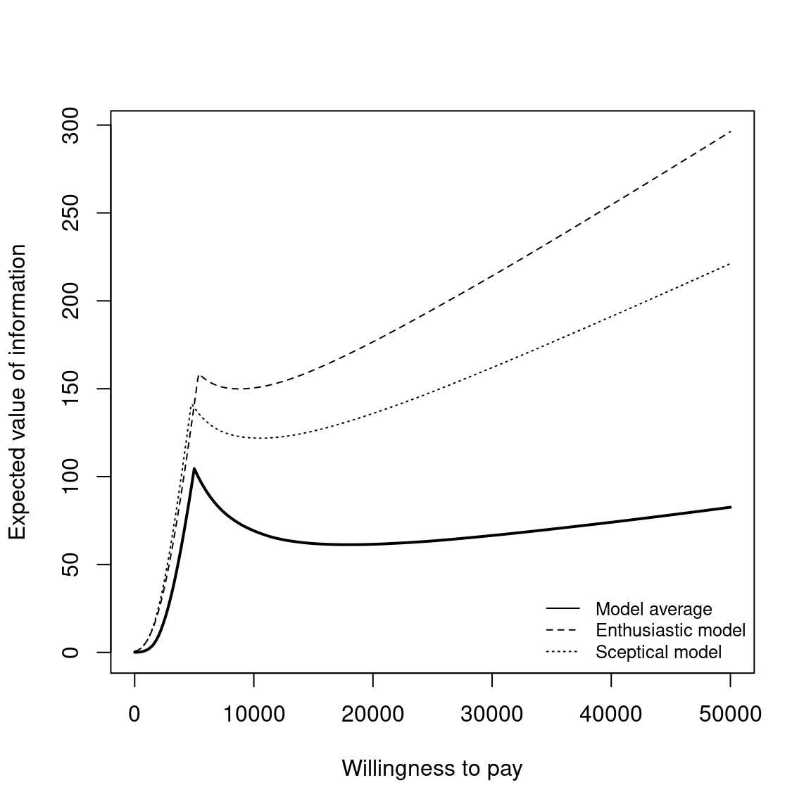
The figures can be obtained by typing the following commands to the R terminal.
# Plot the CEACs
plot(
  m_avg$k, m_avg$ceac,type="l", lwd=2, xlab="Willingness to pay",
  ylab="Probability of cost effectiveness")
points(m_enth$k, m_enth$ceac, type="l", lty=2)
points(m_scep$k, m_scep$ceac, type="l", lty=3)
legend(
  "bottomright", c("Model average","Enthusiastic model","Sceptical model"),
  bty="n", lty=c(1,2,3), cex=.8)

# Plot the EVPPIs
rg <- range(m$evi, m_enth$evi, m_scep$evi)
plot(
  m_avg$k, m_avg$evi, type="l", lwd=2, xlab="Willingness to pay",
  ylab="Expected value of information", ylim=rg)
points(m_enth$k, m_enth$evi, type="l", lty=2)
points(m_scep$k, m_scep$evi, type="l", lty=3)
legend(
  "bottomright", c("Model average","Enthusiastic model","Sceptical model"),
  bty="n", lty=c(1,2,3), cex=.8)
References
Ades, A., Lu, G., Claxton, K., 2004. Expected value of sample information calculations in medical decision modeling. Medical decision making 24, 207–227.
Baio, G., 2012. Bayesian Methods in Health Economics. Chapman Hall/CRC Press, Boca Raton, FL.
Baio, G., Dawid, A.P., 2011. Probabilistic sensitivity analysis in health economics. Stat Methods Med Res. https://doi.org/10.1177/0962280211419832
Box, G., Draper, N., 1987. Empirical Model Building and Response Surfaces. Wiley & Sons, New York, NY.
Briggs, A., Weinstein, M., Fenwick, E., Karnon, J., Schulpher, M., Paltiel, A., 2012. Model Parameter Estimation and Uncertainty: A Report of the ISPOR-SMDM Modeling Good Research Practices Task Force-6. Value in Health 15, 835–842.
Claxton, K., 1999. The irrelevance of inference: a decision-making approach to stochastic evaluation of health care technologies. Journal of Health Economics 18, 342–364.
Hastie, T., Tibshirani, R., 1990. Generalized additive models. CRC Press.
Heath, A., Baio, G., Pechivanoglou, P., 2025. Introduction to Health Technology Assessment, in: Baio, G., Thom, H., Pechivanoglou, P. (Eds.), R for Health Technology Assessment.
Heath, A., Kunst, N., Jackson, C., 2024. Value of information for healthcare decision-making. CRC Press.
Heath, A., Manolopoulou, I., Baio, G., 2017. A review of methods for analysis of the expected value of information. Medical decision making 37, 747–758.
Heath, A., Manolopoulou, I., Baio, G., 2016. Estimating the expected value of partial perfect information in health economic evaluations using integrated nested Laplace approximation. Statistics in Medicine. https://doi.org/10.1002/sim.6983
Heath, A., Strong, M., Glynn, D., Kunst, N., Welton, N.J., Goldhaber-Fiebert, J.D., 2022. Simulating study data to support expected value of sample information calculations: A tutorial. Medical Decision Making 42, 143–155.
Heath, C., A. Jackson, Kunst, N., 2024. Value of information for healthcare decision making. Chapman Hall/CRC Press, Boca Raton, FL.
Hout, B. van, Gordon, M., Rutten, F., 1994. Costs, effects and C/E ratios alognside a clinical trial. Health Economics 3, 309–319.
Lindgren, F., Rue, H., Lindström, J., 2011. An explicit link between Gaussian fields and Gaussian Markov random fields: the stochastic partial differential equation approach. Journal of the Royal Statistical Society: Series B (Statistical Methodology) 73, 423–498.
Philips, Z., Claxton, K., Palmer, S., 2008. The half-life of truth: What are appropriate time horizons for research decisions? Medical Decision Making 28, 287–299.
Rasmussen, C., Williams, C., 2006. Gaussian Processes for Machine Learning. ISBN: 026218253X.
Rue, H., Martino, S., Chopin, N., 2009. Approximate Bayesian Inference for Latent Gaussian Models Using Integrated Nested Laplace Approximations (with discussion). Journal of the Royal Statistical Society B 71, 319–392.
Sadatsafavi, M., Bansback, N., Zafari, Z., Najafzadeh, M., Marra, C., 2013. Need for speed: an efficient algorithm for calculation of single-parameter expected value of partial perfect information. Value in Health 16, 438–448.
Spiegelhalter, D., Abrams, K., Myles, J., 2004. Bayesian Approaches to Clinical Trials and Health-Care Evaluation. John Wiley; Sons, Chichester, UK.
Strong, M., Oakley, J., 2013. An efficient method for computing single-parameter partial expected value of perfect information. Medical Decision Making 33, 755–766.
Strong, M., Oakley, J., Brennan, A., 2014. Estimating Multiparameter Partial Expected Value of Perfect Information from a Probabilistic Sensitivity Analysis Sample A Nonparametric Regression Approach. Medical Decision Making 34, 311–326.
It should be noted that as a result the known-distribution utility function assumes a complex form. For a more complete discussion please see (Baio, 2012).↩︎
We provide these in an
Rfile which is downloadable from this book websitehttp://gianluca.statistica.it/books/bcea/code/chemo_PSA.Rdata.↩︎