2  Case studies

2.1 Introduction

In this chapter, we present the two case studies that are used as running examples throughout the book.

The first example considers a decision-analytic model. This is a popular tool in health economic evaluation, when the objective is to compare the expected costs and consequences of decision options by synthesising information from multiple sources (Petrou and Gray, 2011). Examples of decision-analytic models include decision trees or Markov models. As these models are based on several different sources of information, they can offer decision makers the best avaliable information to reach their decision, as opposed to modelling based on a single randomised clinical trial (RCT). Additionally, RCTs may be limited in scope (\(e.g.\) in terms of the temporal follow up) and thus not be ideal for characterising the long-term consequences of applying an intervention. Thus, even when RCT data are available, a health economic evaluation is often extended to a decision-analytic approach to allow decision makers to capture information about the long-term effects and costs.

The second example is a multi-decision problem. This means that, in contrast to standard economic modelling, where a new intervention \(t=2\) is compared to the status quo \(t=1\), we consider here \(T=4\) potential interventions. This is naturally linked to the wider topic of network meta-analysis (Lu and Ades, 2004), which is an extension of different statistical methods that allow researchers to pool evidence coming from different sources and include direct and indirect comparisons. This is particularly relevant when head-to-head evidence is only available for some of the interventions under consideration. Suitable statistical modelling can be used to infer about the direct comparisons with no information by using the indirect ones.

For both examples, we first introduce the general background, discussing the disease area and the interventions under consideration. We then describe the assumptions underlying the statistical model (\(e.g.\) in terms of distributions for the observed/observable variables and the unobservable parameters). We also show how these can be translated into suitable code to perform a full Bayesian analysis and obtain samples from the relevant posterior distributions (see Section 1.2). Finally, we demonstrate any post-processing required to produce the relevant inputs for the economic model (\(e.g.\) the population average differential of costs and benefits — see Section 1.4). In the rest of the book we refer (rather interchangeably) to OpenBUGS (Lunn et al., 2013) and JAGS (Plummer, 2015), arguably the most popular software to perform Bayesian analysis by means of Markov Chain Monte Carlo simulations.

The examples are then used to showcase the facilities of BCEA and to explain the process of performing an economic evaluation in R, once the statistical model has been fitted. It is important to note (and we will expand on this point in Chapter 3) that BCEA can be used to perform cost-effectiveness analysis when the full statistical model has not been fitted within the Bayesian framework. Nevertheless, we strongly advocate the use of a Bayesian framework and thus we have included these examples to demonstrate a full Bayesian analysis.

Starting from this chapter on the text will include frequent code blocks to show how to execute commands and use the BCEA package. R code is presented in code blocks in the text with a grey background. Indentation indicates lines continuing from the previous statement. Hash symbols (i.e. #) in code blocks indicate comments. In-line words formatted in mono-spaced font (such as this) indicate code, for example short commands or function parameters.

2.2 Preliminaries: computer configuration

In this section we briefly review the ideal computer configuration we are assuming to run the examples later in this chapter and in the rest of the book. It is difficult to guarantee that these instructions will be valid for every future release of the programmes we consider here, although they have been tested under the current releases.

We assume that the user’s computer has the following software installed:

• R and the package BCEA. Other optional packages (\(e.g.\) R2OpenBUGS, R2jags, reshape, plyr or INLA) may need to be installed;
• OpenBUGS or JAGS. These are necessary to perform the full Bayesian analyses we discuss in the rest of the book. It is not necessary to install both;
• The R front-end, for example Rstudio (available for download at the webpage https://www.rstudio.com/. This is also optional and all the work can be done using the standard R terminal;
• A spreadsheet calculator, \(e.g.\) MS Excel or the freely available LibreOffice, which is a decent surrogate and can be downloaded at https://www.libreoffice.org/.

In the following, we provide some general instructions, for MS Windows, Linux or macOS operating systems.

TipInstalling R packages

The “typical” way to install an R package is to use the Comprehensive R Archive Network (CRAN). This is the main repository to which packages are submitted — CRAN does perform a series of checks to ensure that packages meet certain quality standards and function properly across different operating systems and R versions. This generally includes checking code syntax, documentation, examples, as well as running tests within the package itself (if provider by the authors). However, CRAN cannot perform deeper checks on the methodological correctness of the packages that it stores — this is the responsibility of individual authors (and users do help with debugging and reporting potential issues).

There are, however, other ways to distribute and install R packages, some of which are actually very helpful, particularly in development processes. One is to use the R package remotes (Csárdi et al., 2024), which allows the user to install from version-controlling tools such as GitHub. This is relevant, because maintainers can quickly modify packages and use “branches” to produce continuous development of packages — and thus by using this facility, users may have their own customised version of a package, contribute to the development and, in any case, install the most up-to-date development version, if they so wish.

Another helpful tool is provided by the alternative repository available at https://r-universe.dev. This acts very similarly to CRAN, although the process of uploading the packages is perhaps a bit easier and streamlined. While packages may still be hosted under CRAN, as a preference, in their “stable” format, R-universe is often use to allow quicker access to development versions — and for some packages, it represents the main repository at which they are hosted.

2.2.1 MS Windows users

For MS Windows users, the set up should be fairly easy and amounts to the following steps.

1. Download the JAGS Windows installer from the webpage https://sourceforge.net/projects/mcmc-jags/files/JAGS/4.x/Windows/JAGS-4.3.2.exe/download and double-click on the downloaded executable file. Running it will install JAGS on your machine.
2. Download R from https://cran.r-project.org/bin/windows/ (click on the link “install R for the first time”).
   
3. Once you have installed R, open it and type in the terminal the command install.packages("R2jags"). This command will download the package R2jags, which is needed to interface JAGS with R. Follow the on-screen instructions (you will be asked to select a “mirror from which to obtain the file).
   
4. Make sure that the download has worked by typing in the terminal the command library(R2jags). If you do not see any error message, then the package has been successfully installed.
   
5. Install the BCEA package that we will use throughout the practicals, by typing install.packages("BCEA").
   
6. Repeat the installation process for the other packages that are used in the practicals (\(e.g.\) reshape and dplyr). Since this is optional, you can leave this final step to when it is actually needed.

2.2.2 Linux or macOS users

2.2.2.1 Installing R and BCEA

Linux or macOS users should follow slightly different approaches. The installation of R is pretty much the same as for MS WIndows users. From the webpage http://cran.r-project.org/ select your operating system (Linux or macOS) and then your version (eg debian, redhat, suse or ubuntu, for Linux). Follow the instructions to install the software. Once this is done, open R and install the package BCEA by typing at the terminal the command install.packages("BCEA"). You can use similar commands to install other packages.

2.2.2.2 Installing OpenBUGS and JAGS in Linux

While both OpenBUGS and JAGS run natively in Linux (see below for details on how to install them directly), the graphical interface is not available for OpenBUGS.

To install JAGS, depending on your specific distribution of Linux, you may use a very simple command or need to install from source. If you are under Ubuntu or Debian, you can simply type in your terminal:

sudo apt install jags

Alternatively, the source installation (which would work for all Linux distributions) is done following these steps.

1. Go to http://sourceforge.net/projects/mcmc-jags/files/JAGS/4.x/Source/ and download the latest tar.gz file (currently, JAGS-4.3.2.tar.gz)
   
2. Open a terminal window and extract the content of the archive file by typing the command tar xzvf JAGS-4.3.2.tar.gz
   
3. Move to the directory (which has just been created) using the command cd JAGS-4.3.2
   
4. Run the configuration by typing sudo ./configure --prefix=/us && sudo make && sudo make install
   
5. Clean up the unnecessary files and folder by typing cd .. && sudo rm -fr JAGS-4.3.2 && rm JAGS-4.3.2.tar.gz

Either way, if you decide to work with JAGS, then open R and also install the package R2JAGS (using the same command as for the installation of the package R2OpenBUGS). Notice that you don’t have to install both OpenBUGS and JAGS — either is sufficient for the examples shown throughout the book.

Alternatively, you can install the Linux version of OpenBUGS (available from an archived GitHub page) by following the instructions provided. This will work just as well, but you won’t be able to access the graphical interface (which, again, is not really a problem, in our case…).

Warning

NB: Under Linux, you may need to also install additional packages to support the OpenBUGS installation. For instance, under Debian or Ubuntu, you may need to also run in your terminal

sudo apt-get install g++-multilib

to install the library g++multilib.

2.2.2.3 Installing JAGS in macOS

You can install JAGS, following the steps listed below:

1. Install the most recent version of R from the CRAN website.
   
2. (Optional) Download and install RStudio (NB: select the version for the your release of macOS!).
   
3. Install the latest versions of Clang and GNU Fortran from the CRAN tools directory. Note that the most updated release for these may vary so check you select the correct one.
   
4. Now install JAGS version 4.3.2 (JAGS-4.3.2.pkg) from here. Detailed instructions quoted from the JAGS readme file:
   • Download the disk image from the JAGS website.
   • Double click on the disk image to mount (this may not be required).
   • Double click on the JAGS-4.3.2.pkg file within the mounted disk image.
   • Follow the instructions in the installer. If you receive a warning that this software cannot be installed because it comes from an unidentified developer, you need to go to “System Preferences”” > “Security & Privacy”“, and authorize the installation there before proceeding.
   • Authenticate as the administrative user. The first user you create when setting up macOS has administrator privileges by default.
5. Start the Terminal and type jags to see if you receive the message: Welcome to JAGS 4.3.2.
   
6. Open R and install the packages R2jags, coda, R2WinBUGS, lattice, and rjags, by typing install.packages(c("R2jags", "coda", "R2WinBUGS", "lattice", "rjags")) in the R command line.

You may also try installing JAGS on your Mac using MacPorts, by typing in your terminal

sudo apt install jags

to install JAGS.

Alternatively, the source installation (which would work for all Linux distributions) is done following these steps.

1. Go to http://sourceforge.net/projects/mcmc-jags/files/JAGS/4.x/Source/ and download the latest tar.gz file (currently, JAGS-4.3.1.tar.gz)
   
2. Open a terminal window and extract the content of the archive file by typing the command tar xzvf JAGS-4.3.1.tar.gz
   
3. Move to the directory (which has just been created) using the command cd JAGS-4.3.1
   
4. Run the configuration by typing sudo ./configure --prefix=/us && sudo make && sudo make install
   
5. Clean up the unnecessary files and folder by typing cd .. && sudo rm -fr JAGS-4.3.1 && rm JAGS-4.3.1.tar.gz

Either way, if you decide to work with JAGS, then open R and also install the package R2JAGS (using the same command as for the installation of the package R2OpneBUGS). Notice that you don’t have to install both OpenBUGS and JAGS — either is sufficient for the examples shown throughout the book.

2.2.2.4 Installing OpenBUGS in macOS

The installation of OpenBUGS under macOS is slightly more complex, because the process requires some extra software that is not automatically installed. Basically, you need to follow this procedure, as detailed at the website http://www.jkarreth.net/bayes-icpsr.html#bugsmac. You first install a Windows “compatibility layer” (wine), which allows you to run Windows applications on other operating systems. This will also allow you to use the OpenBUGS graphical interface (although, again, we will not, in the practicals!).

1. Update your macOS to the newest version.
   
2. Install Xcode through the App Store.
   
3. Check if you have X11 installed (this is a a windowing system, common on Unix-like operating systems, which, believe it or not, MaxOs is!): hit Command-Space, type X11, and see if the program shows up. If not, install it from here.
   
4. Download a the stable pre-compiled version of wine. Instructions to install wine on macOS are available here.
   
5. Download OpenBUGS323setup.exe (windows executable) and place it in your default directory for wine programs (usually ~/.wine/drive_c).
   
6. Run the OpenBUGS installer:
   • Open XQuartz and a Terminal Window;
   • Move to the directory where you placed the OpenBUGS executable you downloaded in step 2;
   • Type: wine OpenBUGS323setup.exe;
   • Wait for a while and then follow the prompts to install — remember the directory you created to install it (default is ~/[username]/.wine/drive_c/Program Files/OpenBUGS323)
   • NB: There may be an error at the end, this is OK. Close down the Terminal Window
7. It is possible that you need to specify the installation directory to tell your system specifically where to look for BUGS. Typically, this will mean adding the option bugs.directory = "/Users/yourusername/.wine/drive_c/Program Files/OpenBUGS232" (or similar, depending on where you have installed the software!) to the call to the bugs function under R2OpenBUGS. Note that you need to replace “yourusername” with your macOS user name.

Notice that, if you like, you can install R under wine (rather than natively in macOS). Download the MS Windows executable file from CRAN and repeat the instructions above, replacing the command wine OpenBUGS323setup.exe with the command wine R-XXXX.exe, where R-XXXX.exe is the name of the executable file.

Warning

There are some reports that OpenBUGS may fail to work on some macOS versions. Sometimes, when trying to use OpenBUGS from R, it will complain that it can’t find the programme. The bugs function in the R2OpenBUGS package takes an additional input OpenBUGS.pgm, which should be set to the full path to the OpenBUGS executable file. You can try and issue the R command Sys.which("OpenBUGS") at a R terminal and see whether it returns a full path and then pass that string as value for OpenBUGS.pgm, eg if Sys.which("OpenBUGS") returns the string /usr/local/bin/OpenBUGS, then set

bugs(..., OpenBUGS.pgm="/usr/local/bin/OpenBUGS")

2.3 Vaccine

Consider an infectious disease, for instance influenza, for which a new vaccine has been produced. Under the current management of the disease some individuals treat the infection by taking over-the-counter (OTC) medications. Some subjects visit their doctor and, depending on the gravity of the infection, may receive treatment with antiviral drugs, which usually cure the infection. However, in some cases complications may occur. Minor complications will need a second doctor’s visit after which the patients become more likely to receive antiviral treatment. Major complications are represented by pneumonia and can result in hospitalisation and possibly death. In this scenario, the costs generated by the management of the disease are represented by OTC medications, doctor visits, the prescription of antiviral drugs, hospital episodes and indirect costs such as time off work.

The focus is on the clinical and economic evaluation of the policy that makes the vaccine available to those who wish to use it (\(t=2\)) against the null option (\(t=1\)) under which the vaccine will remain unavailable. More details of this example can be found in Baio and Dawid (2011) and references therein.

2.3.1 (Bayesian) Statistical model

2.3.1.1 Assumptions

In a population made of \(N\) individuals, consider the number of patients taking up the vaccine when available \(V_1\sim\mbox{Binomial}(\phi,N)\) where \(\phi\) is the vaccine coverage rate. Obviously, \(V_1=0\) as the vaccine is not available under the status quo. For convenience, we denote the total number of patients in the two groups, vaccinated (\(v=2\)) and non-vaccinated (\(v=1\)), by \(n_{tv}\) with \(n_{t2}:=V_t\) and \(n_{t1}:=N-V_t\) respectively.

The relevant clinical outcomes are: \(j=1\) influenza infection; \(j=2\) doctor visit; \(j=3\) minor complications; \(j=4\) major complications; \(j=5\) hospitalisation; \(j=6\) death; and \(j=7\) adverse events of influenza vaccination. For each clinical outcome \(j\), \(\beta_j\) is its baseline rate of occurrence and \(\rho_{v}\) is the proportional reduction in the chance of infection due to the vaccine. Vaccinated patients (\(v=2\)) will experience a reduction in the chance of infection by a factor \(\rho_2\); conversely, for \(v=1\), individuals are not vaccinated and so the chance of infection is just the attack rate \(\beta_1\). This is equivalent to setting \(\rho_1:=0\).

Under these assumptions, the number of individuals becoming infected in each group is \(I_{tv}\sim\mbox{Binomial}(\pi_v,n_{tv})\), where \(\pi_v := \beta_1(1-\rho_v)\) is the probability of infection. Among the infected subjects, the number visiting a doctor for the first time is \(G\!P^{(1)}_{tv} \sim \mbox{Binomial}(\beta_2,I_{tv})\). Using a similar reasoning, among those who have had a doctor visit, we can define: the number of individuals with minor complications \(G\!P^{(2)}_{tv} \sim \mbox{Binomial}(\beta_3,G\!P^{(1)}_{tv})\); the number of those with major complications \(P_{tv} \sim \mbox{Binomial}(\beta_4,G\!P^{(1)}_{tv})\); the number of hospitalisations \(H_{tv} \sim \mbox{Binomial}(\beta_5,G\!P^{(1)}_{tv})\); and the deaths \(D_{tv} \sim \mbox{Binomial}(\beta_6,G\!P^{(1)}_{tv})\). The number of individuals experiencing adverse events due to vaccination is computed as \(A\!E_{tv} \sim\mbox{Binomial}(\beta_7,n_{tv})\) — obviously, this will be identically 0 under the status quo (\(t=1\)) and among those individuals who choose not to take the vaccine up in the vaccination scenario (\(t=2,v=1\)).

The model also includes other parameters, such as the chance of receiving a prescription after the first doctor visit (\(\gamma_1\)) or following minor complications (\(\gamma_2\)) for a number of antiviral drugs (\(\delta\)); of taking OTC medications (\(\xi\)); and of remaining off-work (\(\eta\)) for a number of days (\(\lambda\)). Combining these with the relevant populations at risk, we can then derive the expected number of individuals experiencing each of these events.

As for the costs, we consider the relevant resources as \(h=1\): doctor visits; \(h=2\): hospital episodes; \(h=3\): vaccination; \(h=4\): time to receive vaccination; \(h=5\): days off work; \(h=6\): antiviral drugs; \(h=7\): OTC medications; \(h=8\): travel to receive vaccination. For each, we define \(\psi_h\) to represent the associated unit cost for which we assume informative lognormal distributions, a convenient choice to model positive, continuous variables such as costs.

Finally, we include in the model suitable parameters to represent the loss in quality of life generated by the occurrence of the clinical outcomes. Let \(\omega_j\) represent the QALYs lost when an individual experiences the \(j-\)th outcome. We assume that doctor visits do not generate loss in QALYs and therefore set \(\omega_2=\omega_3:=0\); the remaining \(\omega_j\)’s are modelled using informative lognormal distributions.

The assumptions encoded by this model are that we consider a population parameter \(\pmb\theta = (\pmb\theta^1,\pmb\theta^2)\), with the two components being defined as \(\pmb\theta^1=(\beta_j,\gamma_1,\gamma_2,\delta,\xi,\eta,\lambda,\psi_h,\omega_j)\) and \(\pmb\theta^2=(\phi,\beta_j,\rho_v,\gamma_1,\gamma_2,\delta,\xi,\eta,\lambda,\psi_h,\omega_j)\). We assume that the components of \(\pmb\theta\) have the distributions specified in Table 2.1, which are derived by using suitable “hyper-parameters” that have been set to encode knowledge \(\mathcal{D}\) available from previous studies and expert opinion. For example, the parameter \(\phi\) identifies a probability (the vaccine coverage) and we may have information about past seasons to suggest that this has been estimated to be between 25 to 63%; this can be translated to a Beta distribution whose parameters can be determined so that roughly 95% of the probability mass lie between these two values. See Baio and Dawid (2011) for a more detailed discussion of this point.

Table 2.1: Distributional assumptions for the model. For each parameter, the distributions are chosen to model the available prior knowledge, represented by existing data or expert opinions. The mathematical form of the distributions is chosen according to the nature of the parameter (i.e. parameters describing probability of occurrence of an event are usually given a Beta distribution), while the values of the hyper-parameters are chosen so that the distribution is consistent with the prior information derived by the clinical literature or expert opinion.

It is easy to check that the assumptions in terms of the interval estimates for the parameters are consistent with the choice of distributions in R, for example using something like the following code.

phi <- rbeta(100000, shape1 = 11.31, shape2 = 14.44)
c(quantile(phi,0.025), quantile(phi,0.5), quantile(phi,0.975))

     2.5%       50%     97.5% 
0.2570468 0.4374178 0.6283160 

2.3.1.2 Coding the assumptions into BUGS/JAGS language

The assumptions and the model structure defined above can be translated into suitable code to perform a MCMC analysis and obtain estimates from the posterior distributions of all the relevant parameters. For example, we could write the following code to be used with OpenBUGS or JAGS.

model {
  # 1. Define the number of people in each group n[v,t],
  #    where t=1,2 is status quo vs vaccination and v=1,2 
  #    is non vaccinated vs vaccinated
  #    t=1: If the vaccine is not available, no one will use it
  #    number of vaccinated in the population 
  V[1] <- 0
  # number of individuals in the two groups
  n[1,1] <- N - V[1]    # non vaccinated
  n[2,1] <- V[1]        # vaccinated
  
  # t=2: When the vaccine is available, some people will 
  # use it but some people won't
  # number of vaccinated in the population 
  V[2] ~ dbin(phi,N)
  # number of individuals in the two groups 
  n[1,2] <- N - V[2]    # non vaccinated
  n[2,2] <- V[2]        # vaccinated
  
  # 2. Vaccination coverage 
  phi ~ dbeta(a.phi, b.phi)
  
  # 3. Probability of experiencing the clinical outcomes 
  #    (in total, N.outcomes = 7)
  #    1. Influenza infection
  #    2. GP visits
  #    3. Minor complications (repeat visit)
  #    4. Major complications (pneumonia)
  #    5. Hospitalisations
  #    6. Death
  #    7. Adverse events due to vaccination
  for (r in 1:4) { 
    beta[r] ~ dbeta(a.beta[r], b.beta[r])
  }
  for (r in 5:6) {
    beta[r] ~ dlnorm(a.beta[r], b.beta[r])
  }
  beta[N.outcomes] ~ dbeta(a.beta[N.outcomes], b.beta[N.outcomes])
  
  # 4. Vaccine effectiveness in reducing influenza (for v=1, it is obviously 0)
  rho[1] <- 0
  rho[2] ~ dlnorm(mu.rho,tau.rho)
  
  
  # 5. Probability of influenza infection
  for (t in 1:2) {
    for (v in 1:2) {
      pi[t,v] <- beta[1]*(1-rho[v])
    }
  }
  
  # 6. Number of patients experiencing events for both 
  #    interventions & compliance groups
  for (t in 1:2) {
    for (v in 1:2) {
      Infected[t,v] ~ dbin(pi[t,v], n[v,t])
      P[t,v] ~ dbin(beta[2], Infected[t,v])
      Repeat.GP[t,v] ~ dbin(beta[3], GP[t,v])
      Pneumonia[t,v] ~ dbin(beta[4], GP[t,v])
      Hospital[t,v] ~ dbin(beta[5], GP[t,v])
      Death[t,v] ~ dbin(beta[6], GP[t,v])
      Trt[1,t,v] ~ dbin(gamma[1], GP[t,v])
      Trt[2,t,v] ~ dbin(gamma[2], Mild.Compl[t,v])
      Mild.Compl[t,v] <- Repeat.GP[t,v] + Pneumonia[t,v]
    }
  }
  Adverse.events ~ dbin(beta[N.outcomes],n[2,2])
  
  # 7. Probability of experiencing other events (impacts on costs and QALYs/QALDs)
  for (i in 1:2) {
    # Treatment with antibiotics after GP visit
    gamma[i] ~ dbeta(a.gamma[i], b.gamma[i])
  }
  # Number of prescriptions of antivirals
  delta ~ dpois(a.delta)
  # Taking OTC
  xi ~ dbeta(a.xi, b.xi)
  # Being off work
  eta ~ dbeta(a.eta, b.eta)
  # Length of absence from work for influenza
  lambda ~ dlnorm(mu.lambda, tau.lambda)
  
  # 8. Costs of clinical resources (N.resources = 8)
  #    1. Cost of GP visit
  #    2. Cost of hospital episode
  #    3. Cost of vaccination
  #    4. Cost of time to receive vaccination
  #    5. Cost of days work absence due to influenza
  #    6. Cost of antiviral drugs
  #    7. Cost of OTC treatments
  #    8. Cost of travel to receive vaccination
  for (r in 1:N.resources) {
    psi[r] ~ dlnorm(mu.psi[r], tau.psi[r])
  }
  
  # 9. Quality of life adjusted days/years loss
  #    1. Influenza infection
  #    2. GP visits (no QALD/Y loss)
  #    3. Minor complications (repeat visit, no QALD/Y loss)
  #    4. Major complications (pneumonia)
  #    5. Hospitalisations (same QALD/Y loss as pneumonia)
  #    6. Death
  #    7. Adverse events due to vaccination
  omega[1] ~ dlnorm(mu.omega[1], tau.omega[1])
  omega[2] <- 0; omega[3] <- 0; 
  for (r in 4:N.outcomes) {
    omega[r] ~ dlnorm(mu.omega[r], tau.omega[r])
  }
}

The model consists of 9 modules as annotated in the code above. Notice that the values of the parameters for each distribution are kept as variables (rather than hard-coded as a fixed number). This is in general a good idea, since changes in the assumed values can be reflected directly using the same code. Of course, this means that the numerical value must be passed to the computer code somewhere else in the scripting process. This, however, helps clarify the whole process and makes debugging easier.

As is possible to see, most of the commands in the BUGS/JAGS language are effectively typed in a way that strongly resembles the standard statistical notation, with the twiddle symbol ~ indicating a stochastic relationship (i.e. a probability distribution), while the assignment symbol <- indicates logical (or deterministic) relationships.

Typically, this code is saved to a text file, for example https://gianluca.statistica.it/books/bcea/code/vaccine.txt. Sometimes, it is helpful to create an R dummy function that contains the model code, e.g.

model = function() {
  for (i in 1:n) {
    y[i] ~ dnorm(mu[i],tau)
    mu[i] <- X[i,] %*% beta
  }
  for (k in 1:K) {
    beta[k] ~ dnorm(0,0.001)
  }
  sigma ~ dexp(3)
  tau <- pow(sigma,-2)
}

The function model contains a hypothetical code for a multivariate linear regression.

It is good practice to store the files in a well-structured set of directories or at least to provide pointers for R so that it can search for the relevant files efficiently. Examples include the directory from which R is launched or alternatively in the directory that is currently in use by R (also termed the “working directory”). The R command

setwd("PATH_TO_RELEVANT_FOLDER")

can be used to set the working directory to any folder, while the command

getwd()
[1] "/home/user/MyStuff"

returns the current (working) directory. Note that R uses Unix-like notation and forward slashes / to separate folders in a text string. Conversely, MS Windows uses backward slashes \ to accomplish the same task. This means that on a MS Windows computer, the working directory will be defined by R as something like

# On a Windows machine:
getwd()
[1] "C:/user/MyStuff"

while the MS Windows notation (\(e.g.\) by copying and pasting the address of the folder from the file explorer) would actually be C:\user\MyStuff. It is thus important to be careful when copying and pasting folder locations from MS Windows into R and the user has two options, both based on Unix-like notation: the first one is to just convert any backward slash to a forward slash. The second option is to escape the backward slashes using a double backward slash (\\), for example as in the following R code.

# On a Windows machine, these two commands are the same:
# 1. using forward slashes
setwd("C:/user/Mystuff)

# 2. using double backward slashes
setwd("C:\\user\\MyStuff")

2.3.1.3 R code to pre-process and load the data

The following R code is used to pre-process and load the data in the R workspace before the model and the health economic analysis can be run. We make use of the utility package bmhe, which can be installed from the R universe and provides a number of utility functions to process the output of Bayesian simulations. To install the package, it is possible to use either of the following commands.

# Installs via the alternative repository at https://giabaio.r-universe.dev/
install.packages(
  "bmhe",
  repos = c("https://giabaio.r-universe.dev","https://cloud.r-project.org")
)

We can then run the following set of commands to create the relevant quantities.

## Loads the values of the hyper-parameters
## (needed to run the Bayesian model using JAGS)
library(bmhe)

# Number of people in the population
N <- 100000 

# Vaccine coverage
phires <- betaPar2(.434, .6, .95)
a.phi <- phires$alpha
b.phi <- phires$beta

# Baseline probabilities of clinical outcomes
# 1. Influenza infection
# 2. GP visits
# 3. Minor complications (repeat visit)
# 4. Major complications (pneumonia)
# 5. Hospitalisations
# 6. Death
# 7. Adverse events due to vaccination
N.outcomes <- 7
mu.beta <- c(.0655,.273,.401,.0128,.00038,.00075)
upp.beta <- c(.111,.51,.415,.0197,.00067,.000132)
sd.beta <- c(NA,NA,NA,NA,.0001,.00028)
a.beta <- b.beta <- numeric()

for (i in 1:4) {
  betares <- betaPar2(mu.beta[i], upp.beta[i], .975)
  a.beta[i] <- betares$alpha
  b.beta[i] <- betares$beta
}
for (i in 5:6) {
  betares2 <- lognPar(mu.beta[i], sd.beta[i])
  a.beta[i] <- betares2$mulog
  b.beta[i] <- 1/betares2$sigmalog^2
}

a.beta[N.outcomes] <- betaPar(.1, .05)$a
b.beta[N.outcomes] <- betaPar(.1, .05)$b

# Decrease in risk of infection due to vaccination
rhores <- lognPar(.69, .05)
mu.rho <- rhores$mulog
tau.rho <- 1/rhores$sigmalog^2

# Treatment with antibiotics after GP visit
mu.gamma <- c(.42, .814);  sd.gamma <- c(.0015, .004)
a.gamma <- b.gamma <- numeric()

for (i in 1:2) {
  gammares <- betaPar(mu.gamma[i], sd.gamma[i])
  a.gamma[i] <- gammares$a
  b.gamma[i] <- gammares$b
}

# Number of prescriptions of antibiotics
a.delta <- 7

# Taking OTC
xires <- betaPar(.95, .005) 
a.xi <- xires$a
b.xi <- xires$b

# Being off work
etares <- betaPar(.9, .005) 
a.eta <- etares$a
b.eta <- etares$b

# Length of absence from work for influenza
lambdares <- lognPar(2.9, 1.25)
mu.lambda <- lambdares$mulog
tau.lambda <- 1/lambdares$sigmalog^2

# Costs (N.resources = 8)
# 1. Cost of GP visit
# 2. Cost of hospital episode
# 3. Cost of vaccination
# 4. Cost of time off for individuals to receive vaccination
# 5. Cost of days work absence due to influenza
# 6. Cost of antibiotics
# 7. Cost of OTC treatments
# 8. Cost of travel to receive vaccination
N.resources <- 8
m.psi <- c(20.66,2656,7.24,10.16,46.27,3.81,1.6,.81)
sd.psi <- c(5.015,440.75,1.81,2.54,11.57,.955,.4,.2)
sd.psi <- .25*m.psi
mu.psi <- tau.psi <- rep(0, N.resources)

for (i in 1:N.resources) {
  psires <- lognPar(m.psi[i], sd.psi[i])
  mu.psi[i] <- psires$mulog
  tau.psi[i] <- 1/psires$sigmalog^2
}

# Quality of life weights (N.outcomes = 7)
# 1. Influenza infection
# 2. GP visits (no QoL loss)
# 3. Minor complications (repeat visit, no QoL loss)
# 4. Major complications (pneumonia)
# 5. Hospitalisations
# 6. Death
# 7. Adverse events due to vaccination
m.omega <- c(4.27,0,0,6.35,6.35,15.29,.55)
sd.omega <- c(1.38,0,0,1.5875,1.5875,3.6,.15)
mu.omega <- tau.omega <- rep(0, N.outcomes)

for (i in c(1,4,5,6,7)) {
  omegares <- lognPar(m.omega[i], sd.omega[i])
  mu.omega[i] <- omegares$mulog
  tau.omega[i] <- 1/omegares$sigmalog^2
}

The very first line of the script loads up the bmhe package. This implements a set of functions and commands that are used throughout the script and thus is fundamental to launch it before the rest of the script can be executed. Although the number of files necessary to run the entire analysis may increase (thus, at face value, increasing the complexity of the process), it is actually good programming practice to use a combination of many smaller, focused scripts, rather than include every commands or functions required in one single, massive file. This, again, makes the process transparent and easier to debug or critically appraise.

The rest of the script defines the values for the parameters used in the distributions associated to the quantities modelled and described above. For example, the function betaPar2 (part of bmhe) can be used to determine the values of the parameters of a Beta distribution so that its average is around 0.436 and 95% of the mass is below the value of 0.6. In particular, running this command on an R terminal gives the following output:

betaPar2(.434, .6, .95)

$alpha
[1] 11.30643

$beta
[1] 14.4411

$theta.mode
[1] 0.434

$theta.mean
[1] 0.4391267

$theta.median
[1] 0.437

$theta.sd
[1] 0.09595895

betaPar2 creates a list of results: the first two elements of the list, alpha and beta are the estimated values of the parameters to be used with a Beta distribution so that roughly 95% of the probability mass is below 0.6. This is in line with the assumptions presented in Table 2.1 for the parameter \(\phi\). Again, we can check the appropriateness of this choice by simply typing the following commands to the R terminal.

phi <- rbeta(100000, 11.30643, 14.4411)
c(quantile(phi,.025), quantile(phi,.5), quantile(phi,.975))

     2.5%       50%     97.5% 
0.2575329 0.4382816 0.6299446 

The other elements of the list are theta.mode, theta.mean, theta.median and theta.sd, which store the values for the mode, mean, median and standard deviation of the resulting Beta distribution. Notice the R “dollar” notation, which can be used to access elements of an object — in other words, if the object x is stored in the R workspace and contains the elements y, z and w, then these can be accessed by using the notation x$y, x$z or x$w.

Another thing to notice is that it is fairly easy to annotate the R code in an informative way. This again increases transparency and facilitates the work of reviewers or modellers called upon a critical evaluation of the analysis process. In line with the point we made above about using many simpler and specific files to execute the several steps of the analysis, rather than one large (and potentially messy) file, it is a good idea to save this code to a script file, say LoadData.R, again assumed to be stored in the working directory. From within the R terminal, the script can be launched and executed by typing the command

source("LoadData.R")

which runs all the instructions in the script sequentially.

2.3.1.4 R code to remotely run BUGS/JAGS and the Bayesian model

At this point, the user is ready to run the model — in a full Bayesian context, this typically means performing a MCMC analysis (see Section 1.2.3) to obtain a sample from the posterior distribution of the random quantities of interest. We reiterate here that these may be unobservable parameters as well as unobserved variables.

R is particularly effective at interfacing with the main software for Bayesian analysis — here we refer to the most popular OpenBUGS (Lunn et al., 2013) and JAGS (Plummer, 2015), but there is a R package to interface with a more recent addition, Stan (Stan development team, 2024). This means that it is possible to produce a set of scripts that can be run in R to pre-process the data, call the MCMC sampler in the background and run the model (written in a .txt file, as shown above) and then post-process the results, \(e.g.\) to obtain the suitable measures of population average costs and effectiveness.

# Define the current as the working directory
working.dir <- paste0(getwd(), "/")

# Load the data into R (assumes the file is stored in the working directory - 
# if not the full path can be provided)
source("https://gianluca.statistica.it/books/bcea/code/LoadData.R")

# Define the file with the model code
download.file(
  url = "https://gianluca.statistica.it/books/bcea/code/vaccine.txt",
  destfile = paste0(working.dir, "code/vaccine.txt")
)
filein <- "code/vaccine.txt"

# Load the package to run OpenBUGS or JAGS from R 
library(R2OpenBUGS)
library(R2jags)

# Define the data list to be passed to BUGS/JAGS
data <- list(
  "N","a.phi","b.phi","mu.rho","tau.rho","a.beta","b.beta","a.gamma",
  "b.gamma","mu.omega","tau.omega","mu.psi","tau.psi","N.outcomes",
  "N.resources","mu.lambda","tau.lambda","a.xi","b.xi","a.eta","b.eta","a.delta"
) 

# Define the quantities to be monitored (stored)
params <- c(
  "beta","phi","omega","rho","Infected","GP","Repeat.GP","Pneumonia",
  "Hospital","Death","Mild.Compl","Trt","Adverse.events","n","gamma",
  "delta","psi","lambda","pi","xi","eta")

# Generate the initial values
inits <- function() {
  list(
    phi = runif(1),
    beta = runif(N.outcomes, 0, 1),
    rho = c(NA, runif(1)),
    gamma = runif(2, 0, 1),
    delta = rpois(1, 2),
    omega = c(runif(1), NA, NA, runif(1), NA, runif(2, 0, 1)),
    psi = runif(N.resources, 0, 10),
    lambda = runif(1),
    eta = runif(1),
    xi = runif(1))
}

# Define the number of iteration, burn-in and thinning, and run BUGS or JAGS
n.iter <- 100000
n.burnin <- 9500
n.thin <- floor((n.iter - n.burnin)/500)

# 1. Run JAGS
vaccine <- jags(
  data, inits, params, model.file=filein, n.chains=2, n.iter,
  n.burnin, n.thin, working.directory=working.dir,
  DIC=FALSE, quiet=TRUE)

# Print the summary stats and attach the results to the R workspace
print(vaccine, digits=3, intervals=c(0.025, 0.975))

Inference for Bugs model at "code/vaccine.txt", 
 2 chains, each with 1e+05 iterations (first 9500 discarded), n.thin = 181
 n.sims = 1000 iterations saved. Running time = 1.191 secs
                   mu.vect  sd.vect       2.5%      97.5%  Rhat n.eff
Adverse.events    4538.277 2650.506   1046.950  10811.150 1.000  1000
Death[1,1]           1.554    1.592      0.000      6.000 1.004   420
Death[2,1]           0.844    1.048      0.000      3.000 1.002  1000
Death[1,2]           0.000    0.000      0.000      0.000 1.000     1
Death[2,2]           0.214    0.510      0.000      1.000 1.003  1000
GP[1,1]           2108.545  955.526    692.950   4582.225 1.001  1000
GP[2,1]           1168.182  567.585    346.975   2514.575 1.000  1000
GP[1,2]              0.000    0.000      0.000      0.000 1.000     1
GP[2,2]            291.191  161.917     83.975    711.075 1.000  1000
Hospital[1,1]        0.808    0.959      0.000      3.000 1.003  1000
Hospital[2,1]        0.457    0.758      0.000      2.000 1.006   790 
...

# In JAGS:
attach.jags(vaccine)

# 2. This runs OpenBUGS
vaccine <- bugs(data, inits, params, model.file=filein, n.chains=2, n.iter,
                n.burnin, n.thin, DIC=FALSE, working.directory=working.dir)

# In OpenBUGS:
attach.bugs(vaccine)

For convenience, we can save them in a file, say code/RunMCMC.R, which can then be run from within the R terminal using the source command.

source("code/RunMCMC.R")

This script proceeds by first loading the relevant packages (which allow R to interface with either OpenBUGS or JAGS); this can be done using the command library(R2OpenBUGS) or library(R2jags), depending on the Bayesian software of choice. Of course, for these to work, either or both OpenBUGS and JAGS need to be installed on the user’s machine (we refer interested readers to the relevant websites, where information is provided on installation and use under different operating systems). In the first part of the script, we also “source” the file LoadData.R, presented above, which prepares the data for either OpenBUGS or JAGS to use. Finally, the current folder is set up as the working directory (but of course, the user can choose any folder for this).

The next step amounts to storing all the relevant input data for the model code into a list. In this case, we need to include all the values for the parameters of the distributions used in the file vaccine.txt, which encodes the model assumptions. Then, we instruct R to read the model assumptions from the file vaccine.txt and finally we define the “parameters” to be monitored. Again, we note that with this terminology we refer to any unobserved or unobservable quantity for which we require inference in the form of a sample from the posterior distribution.

Before we run OpenBUGS or JAGS we need to define the list of “initial values”, which are used to start the Markov chain(s). Notice that both BUGS or JAGS can randomly generate initial values. However, it is generally better to control closely this process (Baio, 2012). This can be done by creating a suitable R function that stores in a list random values for all the quantities that need initialisation. These are obtained by specifying the underlying distribution — for instance, in this case we are generating the initial value for \(\phi\) from a Uniform\((0,1)\) distribution (this is reasonable as \(\phi\) is a probability and so it needs to have a continuous value between 0 and 1). In principle, any quantity that is modelled using a probability distribution and is not observed needs to be initialised. With reference to the model code presented above, it would not possible to initialise the node n[1,2], because it is defined as a deterministic function of other quantities (in this case N and V[2]).

Finally, we define the total number of iterations, the number of iterations to be discarded in the estimate of the posterior distributions (burn-in) and the possible value of the “thinning”. This refers to the operation of only saving one every \(l\) iterations from the Markov Chains. This can help reduce the level of autocorrelation in the resulting chains. For example, we could decide to store 1,000 iterations and obtain this either by saving the last 1,000 runs from the overall process (i.e. by discarding the first 9,000 of the 10,000 iterations produced), or by running the process for 100,000 iterations, discarding the first 9,500 and then saving one every 181 iterations. Of course, the latter alternative involves a longer process just to end up with the same number of samples on which to base the estimation of the posteriors. But the advantage is that it is likely that it will show a lower level of autocorrelation, which means a larger amount of information and thus better precision in characterising the target distributions.

Once these steps have been executed, we can use the commands BUGS or JAGS to run the model. Both would call the relevant MCMC sampler in the background and produce the MCMC estimates. When the process is finished, the user regains control of the R session. A new object, in this case named vaccine, is created in the current workspace. This object can be manipulated to check model convergence, visualise the summary results (using the print method available for both R2OpenBUGS and R2jags) and save the results (i.e. the simulated values from the posterior distributions) to the R workspace.

For example, a summary table can be obtained as follows (here, we only present the first few rows, for simplicity):

print(vaccine, interval=c(.025, .975), digits=3)

Inference for Bugs model at "code/vaccine.txt", 
 2 chains, each with 1e+05 iterations (first 9500 discarded), n.thin = 181
 n.sims = 1000 iterations saved. Running time = 1.191 secs
                   mu.vect  sd.vect       2.5%      97.5%  Rhat n.eff
Adverse.events    4538.277 2650.506   1046.950  10811.150 1.000  1000
Death[1,1]           1.554    1.592      0.000      6.000 1.004   420
Death[2,1]           0.844    1.048      0.000      3.000 1.002  1000
Death[1,2]           0.000    0.000      0.000      0.000 1.000     1
Death[2,2]           0.214    0.510      0.000      1.000 1.003  1000
GP[1,1]           2108.545  955.526    692.950   4582.225 1.001  1000
GP[2,1]           1168.182  567.585    346.975   2514.575 1.000  1000
GP[1,2]              0.000    0.000      0.000      0.000 1.000     1
GP[2,2]            291.191  161.917     83.975    711.075 1.000  1000
Hospital[1,1]        0.808    0.959      0.000      3.000 1.003  1000
Hospital[2,1]        0.457    0.758      0.000      2.000 1.006   790 
...

For each parameter included in the list of quantities to be monitored, this table shows the mean and standard deviation (the columns labelled as mu.vect and sd.vect), together with the 2.5% and 97.5% quantiles of the posterior distributions (which give a rough approximation of a 95% credible interval).

The final columns of the table (indexed by the labels Rhat and n.eff, respectively) present some important convergence statistics. The first one is the potential scale reduction \(\hat{R}\), often termed the Gelman-Rubin statistic. This quantity can be computed when the MCMC process is based on running at least two parallel chains and basically compares the within to the between chain variability. The rationale is that when this ratio is close to 1, then there is some evidence of ‘’convergence’’ because all the chains present similar variability and do not vary substantially among each other, thus indicating that they are all visiting a common area in the parameter’s space. Typically, values below the arbitrary threshold of 1.1 are considered to suggest convergence to the relevant posterior distributions.

The second one is the “effective sample size” \(n_{\textrm{eff}}\). The idea behind this quantity is that the MCMC analysis is based on a sample of n.sims iterations (in this case, this is 1,000). Thus, if these were obtained using a sample of independent observations from the posterior distributions, this would be worth exactly 1,000 data points. However, because MCMC is a process in which future observations depends on the current one, there is some intrinsic “autocorrelation”, which means that often a sample of \(S\) iterations has a value in terms of information that is actually lower. This value is quantified by the effective sample size. When n.eff is close to n.sims, this indicates that the level of autocorrelation is low and that in effect the n.sims points used to obtain the summary statistics are worth more or less their nominal value. On the other hand, when the two are very different this indicates that the MCMC sample contains less information about the posterior.

For example, because of the autocorrelation, the 1,000 simulations used to characterise the posterior distribution of the node Adverse.events are actually equivalent to a sample made by around 310 independent observations from that posterior. In cases such as this, when \(\hat{R}<1.1\) but n.eff is much smaller than n.sims we could conclude that the sample obtained has indeed converged to the posterior distribution but does not contain enough information to fully characterise it. For example, the mean and the central part of the distribution may be estimated with good precision, but the tails may not. One easy (albeit potentially computationally intensive) workaround is to run the MCMC for a (much) longer run and possibly increase the thinning.

Additional analyses to check on convergence may be performed, for example by providing traceplots of the chains, \(e.g.\) as in Figure 1.3 (d), for example using the following command

traceplot(vaccine)

which produces an interactive traceplot for each of the monitored nodes. More advanced graphing and analysis can be done by subsetting the object vaccine and accessing the elements stored therein. Details on how to do this are shown, for example, in Baio (2012).

2.3.2 Economic model

In order to perform the economic analysis, we need to define suitable summary measures of cost and effectiveness. The total cost associated with each clinical resource can be computed by multiplying the unit cost \(\psi_h\) by the number of patients consuming it. For instance, the overall cost of doctor visit is \(\left(G\!P^{(1)}_{tv}+G\!P^{(2)}_{tv}\right)\times \psi_1\). If, for convenience of terminology, we indicate with \(N_{tvh}\) the total number of individuals consuming the \(h-\)th resource under intervention \(t\) and in group \(v\), we can then extend this reasoning and compute the average population cost under intervention \(t\) as \[ c_t := \frac{1}{N}\sum_{v=1}^2 \sum_{h=1}^8 N_{tvh} \psi_h. \tag{2.1}\]

Similarly, the total QALYs lost due to the occurrence of the relevant outcomes can be obtained by multiplying the number of individuals experiencing them by the weights \(\omega_j\). For example, the total number of QALYs lost to influenza infection can be computed as \(I_{tv}\times \omega_1\). If we let \(M_{tvj}\) indicate the number of subjects with the \(j-\)th outcome in intervention \(t\) and group \(v\), we can define the population average measure of effectiveness for intervention \(t\) as \[ e_t := \frac{1}{N}\sum_{v=1}^2 \sum_{j=1}^7 M_{tvj}\omega_j. \tag{2.2}\]

The results of the MCMC procedure used to run the model described above can be obtained by simply running the scripts discussed in Section 2.3.1. However, they are also available in the R object vaccine.RData, which can be directly downloaded at https://gianluca.statistica.it/books/bcea/code/vaccine.RData. They are also part of the BCEA package and are stored in the object vaccine_mat, which is loaded with the dataset Vaccine using the R command data("Vaccine", package="BCEA").

For example, this can be uploaded to the R session by typing the following commands

filepath <- paste0(working.dir, "data/vaccine.RData")

download.file(
  url = "https://gianluca.statistica.it/books/bcea/code/vaccine.RData",
  destfile = filepath)

load(filepath)

ls()

[1] "Adverse.events" "Death"      "GP"             "Hospital"
[5] "Infected"       "N"          "Pneumonia"      "Repeat.GP"
[9] "delta"          "eta"        "gamma"          "lambda"
[13] "n"             "n.sims"     "omega"          "psi"
[17] "xi"

Each of these R objects contains \(n_{\textrm{sims}}=1000\) simulations from the relevant posterior distributions. Before the economic analysis can be run, it is necessary to define the measures of overall cost and effectiveness given in equations Equation 2.1 and Equation 2.2 respectively. This can be done using the results produced by the MCMC procedure with the following R code. Notice that since the utilities are originally defined as quality adjusted life days, it is necessary to rescale them to obtain QALYs.

## Compute effectiveness in QALYs lost for both strategies
QALYs.inf <- QALYs.pne <- QALYs.hosp <- QALYs.adv <- 
  QALYs.death <- matrix(0, nrow = n.sims, ncol = 2)

for (t in 1:2) {
  QALYs.inf[,t] <- ((Infected[,t,1] + Infected[,t,2])*omega[,1]/365)/N
  QALYs.pne[,t] <- ((Pneumonia[,t,1] + Pneumonia[,t,2])*omega[,4]/365)/N
  QALYs.hosp[,t] <- ((Hospital[,t,1] + Hospital[,t,2])*omega[,5]/365)/N
  QALYs.death[,t] <- ((Death[,t,1] + Death[,t,2])*omega[,6])/N
}
QALYs.adv[,2] <- (Adverse.events*omega[,7]/365)/N
e <- -(QALYs.inf + QALYs.pne + QALYs.adv + QALYs.hosp + QALYs.death)

The notation Infected[,t,1] indicates all the simulations (the first dimension of the array) for the t-th intervention (which the for loop sets sequentially to 1 and 2 to indicate \(t=1,2\), respectively) and for the first vaccination group. Similarly, Infected[,t,2] indicates all the simulations for the t-th intervention and for the second vaccination group. Thus, each of these two elements effectively produces the value \(M_{tv1}\) (where \(j=1\) indicates the first outcome) and consequently, the code ((Infected[,t,1] + Infected[,t,2])*omega[,1]/365)/N does identify the quantity \(\frac{1}{N}\sum_{v=1}^{2} M_{tv1}\omega_1\). Following a similar reasoning for all the other outcomes and summing them all up, we do obtain the measure of effectiveness, which is stored in a matrix e with \(n_{\textrm{sims}}\) rows and 2 columns (one for each intervention considered).

We can follow a similar strategy to identify the costs associated with each intervention. First we define the number of “users” (which we indicated earlier as \(N_{tvh}\) and according to the resource depends on the number of doctor (general practitioner) visits, hospitalisations, infections, repeated hospitalisations, or individuals at risk); then we multiply these by the associated cost (contained in the variable psi). Then we sum all the components to derive the overall average cost for each treatment strategy.

## Compute costs for both strategies
cost.GP <- cost.hosp <- cost.vac <- cost.time.vac <- cost.time.off <-
  cost.trt1 <- cost.trt2 <- cost.otc <- cost.travel <- matrix(0, n.sims, 2)

for (t in 1:2) {
  cost.GP[,t] <- (GP[,t,1] + GP[,t,2] + Repeat.GP[,t,1] + 
                    Repeat.GP[,t,2])*psi[,1]/N
  cost.hosp[,t] <- (Hospital[,t,1] + Hospital[,t,2])*psi[,2]/N
  cost.vac[,t] <- n[,2,t]*psi[,3]/N
  cost.time.vac[,t] <- n[,2,t]*psi[,4]/N
  cost.time.off[,t] <- (Infected[,t,1] + Infected[,t,2])*psi[,5]*eta*lambda/N
  cost.trt1[,t] <- (GP[,t,1] + GP[,t,2])*gamma[,1]*psi[,6]*delta/N
  cost.trt2[,t] <- (Repeat.GP[,t,1] + Repeat.GP[,t,2])*gamma[,2]*psi[,6]*delta/N
  cost.otc[,t] <- (Infected[,t,1] + Infected[,t,2])*psi[,7]*xi/N
  cost.travel[,t] <- n[,2,t]*psi[,8]/N
}
c <- cost.GP + cost.hosp + cost.vac + cost.time.vac + cost.time.off + 
  cost.trt1 + cost.trt2 + cost.travel + cost.otc

At this point we are ready to run the Decision Analysis and the Uncertainty Analysis, which BCEA can take care of. We present these parts in Chapter 3 and Chapter 4.

2.4 Smoking cessation

In this example, we will consider a set \(\mathcal{T}=\{t=1,2,3,4\}\) of \(T=4\) potential interventions to help smoking cessation; in particular, \(t=1\) represents no contact (status quo); \(t=2\) is a self-help intervention; \(t=3\) is individual counselling; and \(t=4\) indicates group counselling. The interest is in the joint evaluation of the \(T\) interventions. The analysis will be conducted in the form of a cost-consequence analysis, and as such costs and health effects will not be correlated as it usually happens in the wider framework of a cost-utility analysis. However, it should be noted that there is no substantive difference between a cost-consequence and cost-utility analysis, as argued in Wilkinson (1999). Therefore, the costs and health effects will be analysed separately and then jointly to produce a summary of the comparative cost-effectiveness profiles of the interventions considered.

The available clinical evidence is made by a set of trials in which some combinations of the available interventions have been considered. However, not all the possible pairwise comparisons are observed. The use of a Bayesian model embedding some suitable exchangeability assumptions allows the estimation of a suitable measure of effectiveness for all the interventions (using all the available evidence for each \(t \in \mathcal{T}\)) and for all the possible pairwise comparisons. This is a meta-analysis technique generally referred to as Mixed Treatment Comparison (MTC), which expands the concepts of Bayesian evidence synthesis to generate a network of evidence that can be used to produce the required estimations. More detailed discussion is presented in Welton et al. (2012) and Dias et al. (2013). The data used in this example were originally reported in Hasselblad (1998).

2.4.1 (Bayesian) Statistical model

2.4.1.1 Assumptions

The dataset includes \(N=50\) data points nested within \(S=24\) studies. For each study arm \(i=1,\ldots,N\) we observe a variable \(r_i\) indicating the number of patients quitting smoking out of a total sample size of \(n_i\) individuals. In addition, we also record a variable \(t_i\) taking on the possible values \(1,2,3,4\), indicating the treatment associated with the \(i-\)th data point. The nesting within the trial is accounted for by a variable \(s_i\) taking values in \(1,\ldots,S\).

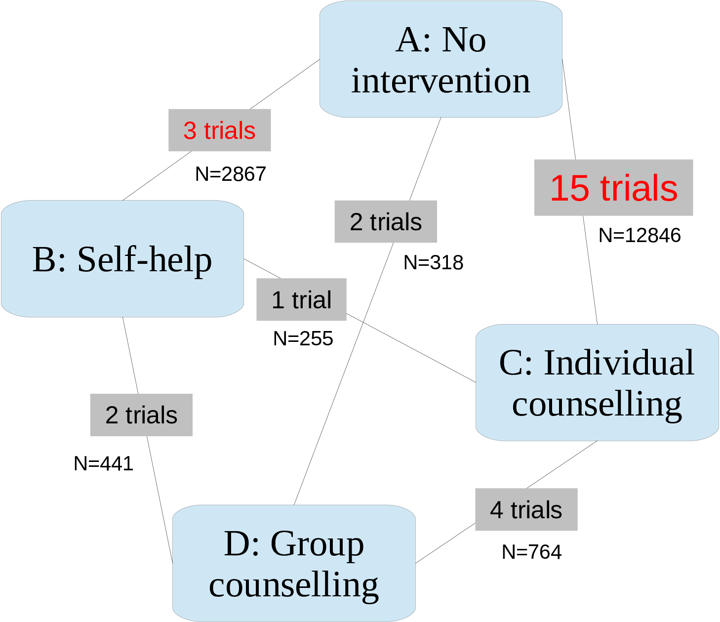
Most studies are simple head-to-head comparisons (i.e. comparing only two interventions), while two of the them are multi-arm trials (the first one involving \(t=1,3,4\), and the second one comparing \(t=2,3,4\)). Most trials compare one of the active treatments \(t=2,3,4\) against the control treatment “No intervention”. Five of the studies consider comparisons between two or more active treatments. The full dataset is presented in Table 2.2.

Table 2.2: The dataset containing information on the \(S=24\) trials on smoking cessation. The data were originally reported in Hasselblad (1998).

Figure 2.1 shows the description of the “network” of data available — the process of combining this information into a consistent framework is often referred to as “Network Meta-Analysis” (NMA).

Figure 2.1: A graphical representation of the network of evidence for the smoking cessation studies

For each study arm we model the number of observed quitters as the realisation of a Binomial random variable: \[ r_{i} \sim \mbox{Binomial}\left(p_{i},n_{i}\right) \] where \(p_i\) is the specific probability of smoking cessation. The main objective of the model is to use the available data to derive a pooled estimation for \(\pi_t\), the intervention-specific probability of smoking cessation.

We use the following strategy. First we model the probabilities \(p_i\) using a structured formulation \[ \mbox{logit}(p_i) = \mu_{s_i}+\delta_{s_i,t_i} \left(1-\mathbb{I}\{t_i=b_{s_i}\}\right) \] The parameter \(\mu_{s_i}\) represents a study-specific baseline value, which is common to all interventions being compared in study \(s_i\). Notice that for each \(i=1,\ldots,N\), \(s_i\) takes on the integer values in \([1;S]\). Thus the vector \(\pmb\mu\) comprises of \(S\) elements.

The parameter \(\delta_{s_i,t_i}\) represents the incremental effect of treatment \(t_i\) with respect to the reference intervention being considered in the study \(s_i\). Specifically, we assume by common convention that the intervention associated with the minimum label value found in each study, is the reference intervention for that study. This formulation allows for a clear specification of study-specific effects and can be easily extended to include study-treatment interaction. The reference (or baseline) intervention for each study is indicated by \(b_{s_i}\); thus \(\delta_{s_i,b_{s_i}}=0\), with the effect of the baseline intervention for each study \(s\) represented by \(\mu_s\). Consequently, in each study \(s\) we assume that the comparator’s effect is the study baseline and that the incremental effect of treatment \(t\) is represented by \(\delta_{s,t}\) if \(t\neq b_s\).

The parameters in \(\pmb\mu\) are given independent minimally informative Normal distributions \(\mu_s \stackrel{iid}{\sim} \mbox{Normal}(0,v)\), where \(v\) is a large fixed value identifying the initial value of the variance of the distributions. On the contrary, we assume that the parameters \(\delta_{s_i,t_i}\) represent “structured” effects \[ \delta_{s_i,t_i} \sim \mbox{Normal}(md_{i}, \sigma^2) \] with \[ md_i = d_{t_i} - d_{b_{s_i}} \] The parameters \(\pmb d=(d_1, \ldots, d_T)\) represent some pooled intervention-specific effect and the mean \(md_i\) is computed as the average difference between the effect for the intervention in row \(i\) and the effect for the reference intervention \(b_{s_i}\) in study \(s_i\). We assume that \(d_1=0\), i.e. that the reference intervention has no effect other than the baseline level, while we model \(d_i \stackrel{iid}{\sim}\mbox{Normal}(0,v)\) for \(i=2,\ldots,T\).

The parameters \(\pmb d\) are defined on the logit scale, and thus in order to compute the estimated probability of smoking cessation on the natural scale for each treatment we need to rescale them. We proceed by estimating the effect for the baseline intervention \(t=1\). Since \(d_1\) was set to \(0\), the treatment effect \(\pi_0\) on the logit scale is given by the average of the baseline effects in the trials including the intervention \(t=1\). The treatment effects \(\pi_t, t=1, \ldots,T\) are calculated as:

\[\begin{align*} & \pi_0 = \dfrac{1}{\sum_{s=1}^S \mathbb{I}\{b_s=1\} } \sum_{s:b_s=1} \mu_s \\ & \text{logit}(\pi_t) = \pi_0 + d_t, \qquad \quad t=1,\ldots,T \end{align*}\]

where \(s:b_s=1\) indicates the subset of studies including the reference intervention arm \(t=1\) as a comparator (baseline). The expression \(\sum_{s=1}^S \mathbb{I}\{b_s=1\}\) indicates the number of studies including treatment \(t=1\), since it is the sum of the indicator function over the trials including that intervention as the baseline comparator.

2.4.1.2 Running the MTC model in JAGS

We run the MTC model in JAGS (although the code presented below will also work in OpenBUGS with only minor modifications — see Section 2.3.1.4). To run the Bayesian evidence synthesis model, it is necessary to store the model specification in a text file that will be then interpreted by JAGS. This file contains the description of the Bayesian model in terms of the stochastic and deterministic relationships between the variables building the model network or graph (more precisely, a direct acyclic graph, or DAG).

The model is an adaptation from the specifications reported by Welton et al. (2012) and Dias et al. (2013). The JAGS code used for the analysis of the smoking cessation data is shown below:

### JAGS model
model {
  for (i in 1:nobs) {
    r[i] ~ dbin(p[i], n[i])
    p[i] <- ilogit(mu[s[i]] + delta[s[i], t[i]])
    delta[s[i], t[i]] ~ dnorm(md[i], tau)
    md[i] <- d[t[i]] - d[b[s[i]]]
  }
  for (i in 1:ns) {
    mu[i] ~ dnorm(0, .0001)
    AbsTrEf[i] <- ifelse(b[i]==1, mu[i], 0)
  }
  pi0 <- sum(AbsTrEf[])/incb
  tau <- pow(sd, -2)
  sd ~ dunif(0.00001, 2)
  d[1] <- 0
  for (k in 2:nt) {
    d[k] ~ dnorm(0, .0001)
  }
  for (j in 1:nt) {
    logit(pi[j]) <- pi0 + d[j]
    for (k in 1:nt) {
      lor[j,k] <- d[j] - d[k]
      log(or[j,k]) <- lor[j,k]
      rr[j,k] <- pi[j]/pi[k]
    }
  }
}

To run the analysis it is necessary to save the model in a plain text file. No specific extensions are required and in this example we will save the file with the name smoking_model_RE.R in the directory from which we run R. We will assume that the csv file containing the data inputs (i.e. smoking_data.csv) is in the same folder. The directory R is using can be displayed using the command getwd() and can be modified by specifying the desired address as the argument of the function setwd, i.e. setwd("PATH_TO_NEW_DIRECTORY").

It is necessary to import the data into R and to pre-process the inputs prior to running the Bayesian model. This can be done by running the following code:

# load the R2jags package and the data file
library(R2jags)

smoking <- read.csv("data/smoking_data.csv", header=TRUE)

# specify the name of the model file
model.file <- "code/smoking_model_RE.txt"

# copy smoking data.frame columns to local variables
nobs <- smoking$nobs; s <- smoking$s; t <- smoking$i;
r <- smoking$r_i; n <- smoking$n_i; b <- smoking$b_i

# number of trials
ns <- length(unique(s))
# number of comparators
nt <- length(unique(t))
# number of observations
nobs <- dim(smoking)[1]
# how many studies include baseline
incb <- sum(table(s,b)[,1] > 0)

The package R2jags is necessary to connect R and JAGS, and is loaded with the command library(R2jags). The command read.csv is used to read into R the data inputs contained in the csv file smoking_data.csv, which will be saved as a data.frame object. Since the quantities need to be available in the R workspace, they are saved as new R variables.

The total number of studies, the arm index for each observation in the respective trial, the number of comparators and observations and the number of trials including the baseline reference treatment, in this case \(t=1\) (no intervention), are also calculated from the data.

The JAGS function used to run the Bayesian evidence synthesis model requires several inputs:

• data: a named list including all the inputs needed by the model;
• inits: a list of initial values or a function generating the initial values for (a subset of) the stochastic parameters in the model. In this example we set inits to NULL, which means that JAGS will choose at random the initial values for all the parameters in the model. The initial values of the parameters will be randomly drawn from the space of values they can assume, determined by their stochastic definition;
• parameters.to.save: a vector of variables to monitor, i.e. the parameters of interest. JAGS will save the output of the simulations from the associated posterior distributions only of the monitored parameters;
• model.file: the name or address of the file containing the model. Since we previously saved the model in the R as the file smoking_model_RE.R, the name of this file will be the value passed to this argument;
• n.chains: the number of parallel Markov chains to run. It is highly recommended that these are at least 2, to allow for checking the convergence and the mixing of the chains;
• n.iter: the number of iterations to perform for each chain from initialisation;
• n.thin: the thinning rate, i.e. after how many iterations a single value form the posterior distribution is saved, discarding the others;
• n.burnin: the length of the burn-in, i.e. the number of simulations to discard after the initialisation of the chains before saving any value. If not specified as in this case, by default it is set to n.iter/2.

More details on how to run a JAGS model and then post-process its results for the purposes of health economic analysis are given in Baio (2012).

At this point, all the necessary data inputs have been pre-processed and it is possible to run the MTC analysis model:

# Define the current as the working directory
working.dir <- paste0(getwd(), "/")

# define data and parameters to monitor
inputs <- list("s","n","r","t","ns","nt","b","nobs","incb")

pars <- c("rr","pi","p","d","sd")

smoking_output <- jags(
  data=inputs, inits=NULL, parameters.to.save=pars, model.file=model.file,
  working.directory=working.dir, n.chains=2, n.iter=20000, n.thin=10, DIC = TRUE,
  quiet = TRUE, progress.bar = "none")

The JAGS function will save the output of the model in the rjags object which we called smoking_output. A summary of the model results can be printed out by executing the following line of code:

print(smoking_output)

Inference for Bugs model at "code/smoking_model_RE.txt", 
 2 chains, each with 20000 iterations (first 10000 discarded), n.thin = 10
 n.sims = 2000 iterations saved. Running time = 2.254 secs
         mu.vect sd.vect    2.5%     25%     50%     75%   97.5%  Rhat n.eff
d[1]       0.000   0.000   0.000   0.000   0.000   0.000   0.000 1.000     1
d[2]       0.508   0.417  -0.337   0.238   0.514   0.776   1.333 1.031    77
d[3]       0.868   0.251   0.404   0.695   0.856   1.024   1.400 1.001  2000
d[4]       1.122   0.434   0.316   0.825   1.109   1.401   1.979 1.004   420
p[1]       0.060   0.018   0.031   0.047   0.059   0.071   0.100 1.001  2000
p[2]       0.155   0.030   0.101   0.134   0.153   0.174   0.220 1.001  2000
p[3]       0.086   0.023   0.048   0.070   0.084   0.100   0.135 1.001  2000
p[4]       0.134   0.036   0.071   0.108   0.131   0.156   0.211 1.001  2000
p[5]       0.144   0.035   0.083   0.120   0.142   0.166   0.220 1.001  2000
p[6]       0.174   0.028   0.124   0.155   0.173   0.192   0.233 1.004   490
p[7]       0.106   0.011   0.085   0.098   0.105   0.113   0.128 1.001  1600 
...

The table above reports for each monitored variable the estimated mean, standard deviation, several percentiles of the posterior distributions (2.5%, 25%, 50%, 75% and 97.5%), the convergence Gelman-Rubin \(\widehat{R}\) diagnostic and the effective sample size n.eff. The latter gives an indication of the presence of auto-correlation within the chains by quantifying the information contained in the vector of simulations used to estimate every parameter. The percentiles can be used to approximate a credible interval (CrI), which is an interval of values containing a posterior probability mass equal to 0.95; assuming the unimodality of the distributions (as it is the case), the posterior 95% CrI can be approximated by taking the 2.5% and 97.5% percentiles as the lower and upper bound, respectively.¹

The diagnostics measures indicate a good convergence of the model, with the Gelman-Rubin \(\widehat{R}\) statistics being below 1.1 for all the measures. In addition the effective sample size does not signal the presence of auto-correlation within the chains.

From this output we can observe that the most effective treatment is \(t=4\) (Group counselling) with an associated probability of patients quitting smoking equal to \(\pi_4=0.17\) (95% CrI [0.09; 0.29]). It is followed by: \(t=3\) (Individual counselling) associated with a probability of quitting of \(\pi_3=0.13\) (95% CrI [0.10; 0.17]); \(t=2\) (Self-help) with a probability of \(\pi_2=0.10\) (95% CrI [0.05; 0.17]); and lastly \(t=1\) (No intervention) with an estimated probability of quitting equal to 0.06 (95% CrI [0.04; 0.09]). The results are represented graphically in Figure 2.2. It can be observed that the uncertainty associated with the effect size of group counselling is high, with a 95% credible interval wider than the ones for the other interventions.

Figure 2.2: Mean and 95% credible intervals (CrI) of the re-estimated treatment effects of each treatment. Group counselling resulted in having the best estimated efficacy, followed by individual counselling, self-help and no intervention. The credible interval associated with the group counselling estimate was substantially wider than the ones for the other comparators.

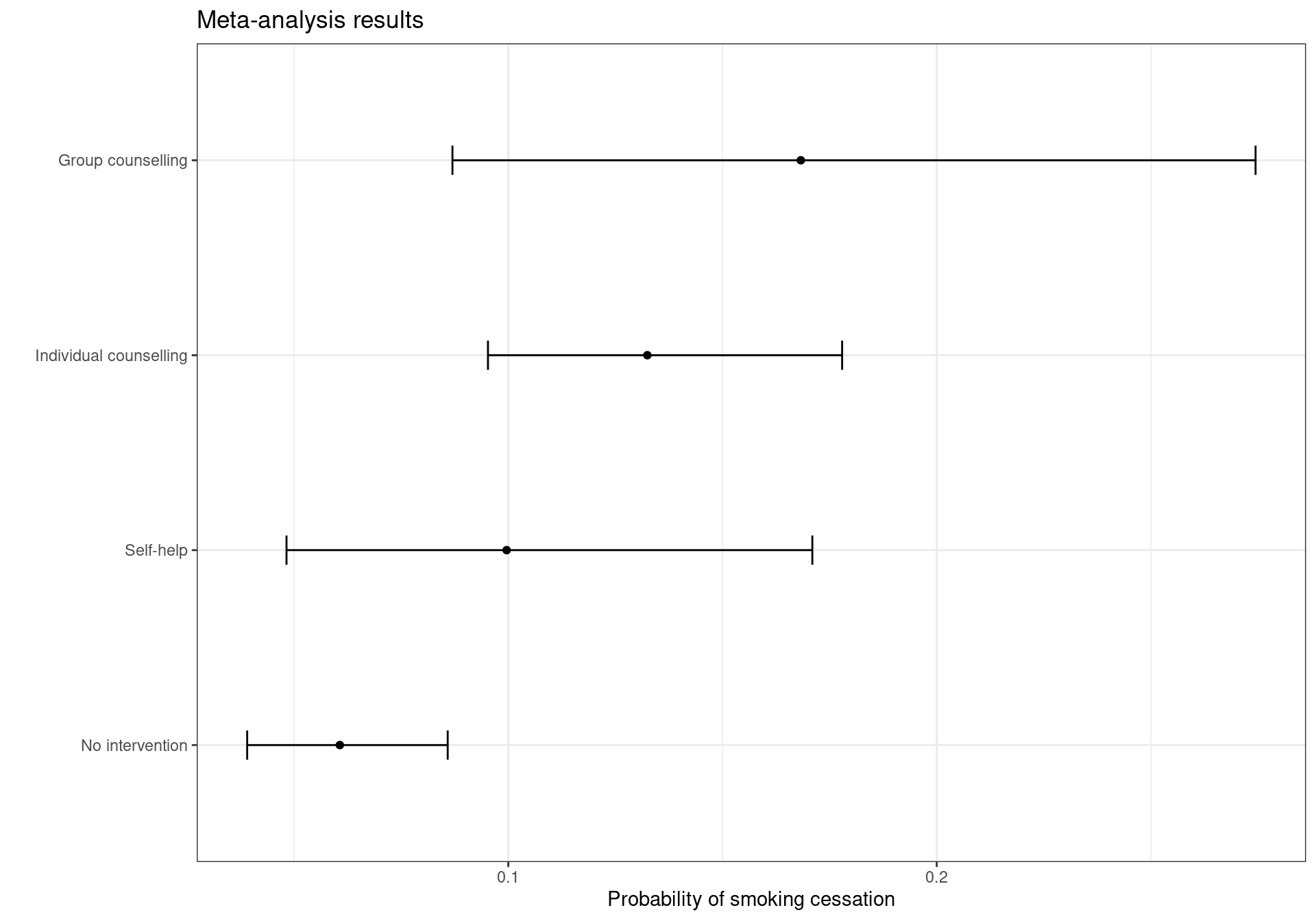
The plot in Figure 2.2 can be reproduced using the following code:

library(ggplot2)

attach.jags(smoking_output)
tr.eff <- data.frame(t(apply(pi, 2, quantile, c(0.025, 0.975))))
names(tr.eff) <- c("low", "high")
treats <- c(
  "No intervention", "Self-help", "Individual counselling", "Group counselling")
tr.eff <- cbind(
  tr.eff, mean=smoking_output$BUGSoutput$mean$pi, 
  interventions=factor(treats, levels=treats)
)
detach.jags()

ggplot(tr.eff) + geom_point(aes(y=mean, x=interventions)) +
  geom_errorbar(aes(x=interventions, ymin=low, ymax=high), width=0.15) +
  labs(
    x="", y="Probability of smoking cessation", title="Meta-analysis results") +
  coord_flip() + theme_bw()

The simulations from the posterior distributions of the parameters that will be used in the economic model are stored in the BUGSoutput element of the rjags output object. The vectors of simulations can be attached to the current workspace by using the command attach.jags, which makes the values available in the workspace². As the economic model will be based on the 1,000 values obtained in JAGS, it is necessary to extract these values from the output object. In the following code, we attach the JAGS output to the workspace and copy the values simulated from the posterior distributions of the estimated probability of cessation for each treatment \(\pmb{\pi} = (\pi_1,\pi_2,\pi_3,\pi_4)\) in a \(2000 \times 4\) matrix to pi_samples. We do this because pi is a built-in constant representing the mathematical constant \(\pi\) and it is good practice to avoid overwriting these and avoiding any problems later on. The variable pi_samples will be used as inputs for the economic model.

attach.jags(smoking_output)
pi_samples <- pi

2.4.2 Economic model

Similarly to the Vaccine example, we need now to include other variables and, generally, post-process the output of the Bayesian model to obtain the quantities necessary to perform the Decision and Uncertainty Analyses.

For example, in this case no data on the costs were provided in addition to the effectiveness reported in Hasselblad (1998). Thus, for the purposes of this example, we extracted information published in McGhan and Smith (1996), who reported costs for different class of interventions for smoking cessation. The costs in British pounds were taken from Flack et al. (2007). Although the interventions reported in Hasselblad (1998) were not described in detail, a comparison of the meta-analysis results with the comparative efficacy measures given in McGhan and Smith (1996) showed consistent results, indicating substantial similarity between the interventions in the two studies.

The costs for the comparators included in the analysis are defined as follows:

1. No intervention:

• No costs: £0;

2. Self-help:

• Nicotine replacement therapy (NRT) for five weeks (35 patches at £1.30 each);

3. Individual counselling:

• NRT for five weeks (35 patches at £1.30 each);
• Five clinic visits (£10.00 each);

4. Group counselling:

• NRT for five weeks (35 patches at £1.30 each);
• Five group visits (£19.46 each).

The total average costs per intervention were: £0 for \(t=1\); £45.50 for \(t=2\); £95.50 for \(t=3\); and £142.80 for \(t=4\). Due to the expected variability associated to the compliance to the interventions in general practice and to the potential need of additional counseling and pharmacological treatment for some patient, it is reasonable to describe the uncertainty associated with the costs with a probability distribution.

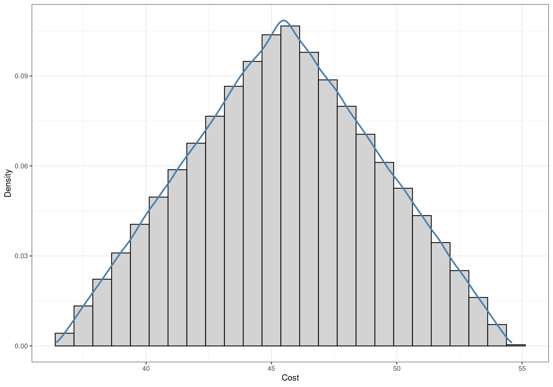
For simplicity, a triangular distribution is associated with all treatment costs (excluding the reference “No intervention” comparator), with limits defined by the average intervention cost \(\pm30\%\). The triangular distribution is a triangle-shaped curve with a null associated density of probability outside the specified lower and upper bounds. It increases linearly from the lower bound to its mode, and decreases linearly up to the upper limit. A graphical representation is given in Figure 2.3. A real-world analysis could be based on more appropriate assumptions for the cost distributions.

Figure 2.3: The distribution represents the uncertainty associated with the costs for the self-help intervention. The curve is shaped as a triangle, hence its name. In this case the mean is equidistant to the lower and upper bound, thus corresponding to the mean (and median) of the distribution.

The distributions of the costs need to be simulated to be inputted in the cost-effectiveness model. The reference comparator \(t=1\) is assumed not to have an associated costs, i.e. its cost is always null. In formal terms, a degenerate probability distribution which assumes the value zero with probability equal to one is assigned to this parameter. The costs for the other interventions are simulated from the intervention-specific triangular distributions described above. Functions to sample from a triangular distribution are not included in the default libraries of R, thus the triangle package needs to be installed to use the following code. The package is available on CRAN, and can be installed as usually from a GUI or by inputting the following command:

install.packages("triangle")

The code to obtain the simulated values from the probability distributions of the costs, stored in the cost matrix, is presented below. Since we populated the matrix with zeroes when creating the object, the costs for \(t=1\) are automatically assigned. The function rtriangle accepts as arguments the number of simulations needed, the lower bound of the distribution a and the upper bound b. If not specified, the mode of the distribution c is calculated by default as the average of the two extremes; since we are using symmetric distributions and thus the mode corresponds to the mean, there is no need to specify this parameter.

library(triangle)

cost.t1 <- 45.5
cost.t2 <- 95.5
cost.t3 <- 142.8

c <- matrix(data=0, nrow=1000, ncol=4)
c[,2] <- rtriangle(1000, a=cost.t1*.8, b=cost.t1*1.2)
c[,3] <- rtriangle(1000, a=cost.t2*.8, b=cost.t2*1.2)
c[,4] <- rtriangle(1000, a=cost.t3*.8, b=cost.t3*1.2)

As for the measure of effectiveness, we can use data from Taylor et al. (2002) on the increments in life expectancy gained. The authors analysed the increments in life expectancy observed in a US survey, reported in Table 2.3.

Table 2.3: Life expectancy increments gained by smoking cessations per gender and age at quitting. Source: Taylor et al. (2002).

Age at quitting	Men	Women
35	8.5	7.7
45	7.1	7.2
55	4.8	5.6
65	4.6	5.1

Data on the prevalence of smoking in the British setting were obtained from the 2013 report of the charity Action on Smoking and Health (ASH, ASH: Action on Smoking and Health, 2013). The data have been summarised in Table 2.4. A split by both gender and age was not included, but the overall proportions of men and women smoking were reported as 22% and 20% in 2012, respectively. This means that the proportion of men among smokers was 52%. It has been assumed that the proportion was not different among the age groups due to lack of data.

Table 2.4: Proportion of smokers per age group. The data on smoking statistics have been published by the charity Action on Smoking and Health in October 2013, reporting the prevalence of cigarette smoking in the UK. Source ASH: Action on Smoking and Health (2013).

The distribution by age of the population in the UK was taken from the 2011 census by the Office of National Statistics (ONS). The data tables are available from the ONS website³.

The data for the life years gained reported in Taylor et al. (2002) did not include individuals younger than 35 or older than 65 years. For simplicity, we assume here that the gain for quitters younger than 35 years was the same observed for the quitters at 35 years and that individuals aged 65 to 80 years quitting had the same gain as 65 years old quitters (Table 2.5).

Table 2.5: Data inputs for the simulation of life years gained by smoking cessation. The dataset is contained in the file smoking_cessation_simulation.csv, available at the website https://gianluca.statistica.it/books/bcea/code/smoking_cessation_simulation.csv

The average life expectancy was calculated using a simulation-based approach. For each of the 1,000 simulations, 1,000 smoking individuals were drawn from the distribution of smokers per age, calculated on the basis of the age distribution in the UK and the proportion of smokers per age group. The gender was simulated from a Binomial model based on the split reported in the ASH smoking statistics and the life years reported in Taylor et al. (2002) were assigned.

To obtain the 1,000 simulations from the posterior distribution of the average life years gained by quitters, the code below has been used. Notice that, in order to use the code, the file smoking_cessation_simulation.csv needs to be available in the same directory from which R is run, or the correct address to the file needs to be specified. Each of the 1,000 individuals in the cohorts are associated with a simulated age. This is drawn from a Multinomial distribution with a vector of probabilities equal to the observed frequency for each age group. The gained life years are calculated for each group based on the gender split. The results are then averaged over the sample, to obtain a vector composed by 2,000 elements. To repeat the process 4 times, obtaining 2,000 simulations for each treatment, 8,000 samples from the Multinomial distribution are taken. These are successively arranged in a matrix with 2,000 rows and 4 columns.

data <- read.csv(file="data/smoking_cessation_simulation.csv")
life.years <- with(data, rmultinom(n = 2000*4, size = 1000, prob = pr.age) * 
                     (.52*Male.ly + .48*Female.ly))

life.years <- matrix(apply(life.years, 2, sum)/1000, 
                     nrow=2000, ncol=4)

At this point it is possible to obtain the life years gained for each intervention. It is only necessary to multiply the probability of smoking cessation \(\pi\) for each treatment by the average number of life years gained by quitting. This can be obtained by a multiplication of the two quantities. The following code creates the effectiveness variable and visualises the first few rows.

e <- pi_samples*life.years
head(e)

          [,1]      [,2]      [,3]      [,4]
[1,] 0.4854891 0.6120225 0.8054989 0.8421482
[2,] 0.4297074 0.4871880 0.8423246 0.7924177
[3,] 0.4288873 0.6058611 0.8286283 1.5606504
[4,] 0.5311160 0.7163197 0.9238518 1.0447437
[5,] 0.4302787 0.4126161 0.9960491 1.0501767
[6,] 0.4109948 0.5318390 1.0978298 1.4824486

Again, this process is completed by running BCEA and performing the Decision and Uncertainty Analysis (as described in details in Chapter 3 and Chapter 4).

References

ASH: Action on Smoking and Health, 2013. ASH fact sheet on smoking statistics.

Baio, G., 2012. Bayesian Methods in Health Economics. Chapman Hall/CRC Press, Boca Raton, FL.

Baio, G., Dawid, A.P., 2011. Probabilistic sensitivity analysis in health economics. Stat Methods Med Res. https://doi.org/10.1177/0962280211419832

Csárdi, G., Hester, J., Wickham, H., Chang, W., Morgan, M., Tenenbaum, D., 2024. remotes: R Package Installation from Remote Repositories, Including ’GitHub’.

Dias, S., Welton, N.J., Sutton, A.J., Ades, A.E., 2013. Technical support documents: Evidence synthesis series. National Institute for Health; Care Excellence (NICE), Decision Support Unit.

Flack, S., Taylor, M., Trueman, P., 2007. Cost-effectiveness of interventions for smoking cessation. York Health Economics Consortium.

Gelman, A., Carlin, J., Stern, H., Dunson, D., Vehtari, A., Rubin, D., 2013. Bayesian Data Analysis - 3rd edition. Chapman Hall/CRC, New York, NY.

Hasselblad, V., 1998. Meta-analysis of multitreatment studies 18, 37–43.

Lu, G., Ades, A., 2004. Combination of direct and indirect evidence in mixed treatment comparisons. Statistics in Medicine 23, 3105–3024.

Lunn, D., Jackson, C., Best, N., Thomas, A., Spiegelhalter, D., 2013. The BUGS book – a practical introduction to Bayesian analysis. Chapman Hall/CRC, New York, NY.

McGhan, W.F.D., Smith, M., 1996. Pharmacoeconomic analysis of smoking-cessation interventions. Am J Health-Syst Pharm 53, 45–52.

Petrou, S., Gray, A., 2011. Economic evaluation using decision analytical modelling: Design, conduct, analysis, and reporting. British Medical Journal 342. https://doi.org/http://dx.doi.org/10.1136/bmj.d1766

Plummer, M., 2015. JAGS: Just Another Gibbs Sampler, version 4.0.0.

Stan development team, 2024. Stan Modeling Language Users Guide and Reference Manual. https://mc-stan.org.

Su, Y.-S., Yajima, M., 2012. R2jags — a package for running jags from R.

Taylor, D.H., Jr, Hasselblad, V., Henley, S.J., Thun, M.J., Sloan, F.A., 2002. Benefits of smoking cessation on longevity 92.

Welton, N.J., Sutton, A.J., Cooper, N.J., Abrams, K.R., Ades, A.E., 2012. Evidence synthesis for decision making in healthcare. John Wiley & Sons, Ltd.

Wilkinson, D., 1999. Cost-benefit analysis versus cost-consequences analysis. Performance Improvement Quarterly.

---

1. It should be noted that the estimation of the ‘’effective number of parameters’’ \(p_D\) is controversial. The definition reported in Gelman et al. (2013) and in Lunn et al. (2013), which is also the one adopted in BUGS, should be preferred instead of the one reported by R2jags (Su and Yajima, 2012). This statistic is calculated by R2jags as: \(p_D = \mbox{Var}[\bar{D}_{model}]/2\) while both Gelman et al. (2013) and Lunn et al. (2013) report that the preferred definition is: \(p_D = \bar{D}_{model} - D(\widehat{\theta})\) where \(\bar{D}_{model}\) is the posterior deviance of the model and \(D(\widehat{\theta})\) is the deviance in correspondence of the estimated posterior mean of the vector of parameters \(\theta\). It should be noted that the definition of \(p_D\) has a direct impact on the deviance information criteria (DIC), which is an index commonly used for model comparisons, defined as \(\text{DIC} = \bar{D}_{model} + p_D = D(\widehat{\theta}) + 2p_D\).

2. When using OpenBUGS and R2OpenBUGS, the object can be attached to the R workspace using the command attach.bugs(object) or attach.jags(object), respectively.

3. At the address https://www.ons.gov.uk/census/2011census/2011censusdata/2011censusdatacatalogue