1 Bayesian analysis in health economics
1.1 Introduction
Modelling for economic evaluation of health-care data has received much attention in both the health economics and the statistical literature in recent years (Briggs et al., 2006; Willan and Briggs, 2006), increasingly often under a Bayesian statistical approach (Baio, 2012; O’Hagan et al., 2001; O’Hagan and Stevens, 2001; Spiegelhalter et al., 2004).
Generally speaking, health economic evaluation aims at comparing the economic performance of two or more alternative health interventions. In other words, the objective is the evaluation of a multivariate outcome that jointly accounts for some specified clinical benefits or consequences and the resulting costs. From the statistical point of view, this is an interesting problem because of the generally complex structure of relationships linking the two outcomes. In addition, simplifying assumptions, such as (bivariate) normality of the underlying distributions are usually not granted (we return to this point later).
In this context, the application of Bayesian methods in health economics is particularly helpful because of several reasons:
- Bayesian modelling is naturally embedded in the wider scheme of decision-theory; ultimately, health economic evaluations are performed to determine the optimal course of actions in the face of uncertainty about the future outcomes of a given intervention, both in terms of clinical benefits and the associated costs.
- Bayesian methods allow extreme flexibility in modelling, especially since the application of revolutionary computational methods such as Markov Chain Monte Carlo has become widespread. This is particularly relevant when the economic evaluation is performed by combining different data into a comprehensive decision model.
- Sensitivity analysis can be performed in a straightforward way under the Bayesian approach and can be seen as a by-product of the modelling strategy. This is extremely helpful in health economics, as decisions are often made on the basis of limited evidence. For this reason, it is essential to understand the impact of model and parameter uncertainty on the final outputs.
This chapter is broadly divided in two main parts. The first one introduces the main aspects of Bayesian inference (in Section 1.2). First, in Section 1.2.1 we introduce the main ideas underlying the Bayesian philosophy. We then present the most important practical issues in modelling in Section 1.2.2 and computation in Section 1.2.3.
The second part of the chapter is focused on presenting the basics of health economic evaluation in Section 1.3 and then the practical aspects of this process are presented in Section 1.4 which introduces the process of health economic evaluation from the Bayesian point of view.
1.2 Bayesian inference and computation
1.2.1 Bayesian ideas
In this section we briefly review the main features of the Bayesian approach to statistical inference as well as the basics of Bayesian computation. A detailed presentation of these subtle and important topics is outside the scope of this book and therefore we only briefly sketch them here and refer the reader to Bernardo and Smith (1999); Lindley (2000); Robert (2001); Spiegelhalter et al. (2004); Lindley (2006); Carlin and Louis (2009); Jackman (2009); Christensen et al. (2011); Gelman et al. (2013); Lunn et al. (2013); Kruschke (2015); McElreath (2015).
A Bayesian model specifies a full probability distribution to describe uncertainty. This applies to data, which are subject to sampling variability, as well as to parameters (or hypotheses), which are typically unobservable and thus are subject to epistemic uncertainty (\(e.g.\) the experimenter’s imperfect knowledge about their value) and even future, yet unobserved realisations of the observable variables (data, Gelman et al., 2013).
As a consequence, probability is used in the Bayesian framework to assess any form of imperfect information or knowledge. Thus, before even seeing the data, the experimenter needs to identify a suitable probability distribution to describe the overall uncertainty about the data \(\pmb y\) and the parameters \(\pmb \theta\). We generally indicate this as \(p(\pmb y, \pmb\theta)\). By the basic rules of probability, it is always possible to factorize a joint distribution as the product of a marginal and a conditional distribution. For instance, one could re-write \(p(\pmb y,\pmb\theta)\) as the product of the marginal distribution for the parameters \(p(\pmb{\theta})\) and the conditional distribution for the data, given the parameters \(p(\pmb y \mid \pmb{\theta})\). But in exactly the same fashion, one could also re-express the joint distribution as the product of the marginal distribution for the data \(p(\pmb y)\) and the conditional distribution for the parameters given the data \(p(\pmb{\theta} \mid \pmb y)\). Consequently, \[ p(\pmb y,\pmb{\theta}) = p(\pmb\theta)p(\pmb y\mid \pmb{\theta}) = p(\pmb y)p(\pmb{\theta} \mid \pmb y) \]
from which Bayes’ Theorem follows in a straightforward way: \[ p(\pmb \theta \mid \pmb y) = \frac{p(\pmb \theta)p(\pmb y \mid \pmb\theta)}{p(\pmb y)}. \tag{1.1}\]
While mathematically incontrovertible, Bayes’ Theorem has deeper philosophical implications, which have led to heated debates, within and without the field of Statistics. In fact, the qualitative implications of this construction are that, if we are willing to describe our uncertainty on the parameters before seeing the current data through a probability distribution, then we can update this uncertainty by means of the evidence provided by the data into a posterior probability, the left hand side of Equation 1.1. This allows us to make inference in terms of direct probabilistic statements.
In fact, a truly “hard-core” Bayesian analysis would not even worry about parameters but would rather model directly the observable variables (\(e.g.\) produce a marginal model for the data only). In any case, it is possible to evaluate probabilistically unobserved data \(\tilde{\pmb y}\), assumed to be of the same nature as those already observed by means of the (posterior) predictive distribution \[ p(\tilde{\pmb y}\mid \pmb y) = \int p(\tilde{\pmb y}\mid \pmb\theta)p(\pmb\theta\mid\pmb y)\mbox{d}\pmb\theta. \tag{1.2}\]
Looking at Equation 1.1 and Equation 1.2 it should be clear that, in a Bayesian analysis, the objective is to evaluate the level of uncertainty on some target quantity (be it the unobservable parameter \(\pmb \theta\) or the the unobserved variable \(\tilde{\pmb y}\)), given the inputs, \(i.e.\) the observed data \(\pmb y\) and the set of assumptions that define the model in question.
Crucially, the Bayesian approach correctly recognises that, once the data have been observed, there is no uncertainty left on their realised value. Unlike classical statistical methods, what values might have been observed and how likely they might have been under the specified model are totally irrelevant concepts1.
In a Bayesian context, inference directly involves the quantities that are not observed — and again there is no distinction in the quantification of the uncertainty about their value depending on their nature (\(i.e.\) parameters or future data). A Bayesian analysis aims at revising the level of uncertainty in light of the evidence that has become available: if data \(\pmb y\) are observed, we move from a prior to a posterior state of knowledge/uncertainty.
1.2.2 Specifying a Bayesian model
When conducting a real-life Bayesian analysis, one has to think carefully about the model used to represent not only sampling variability for the observable data, but also the relevant parameters2.
We note here that, in some sense, modelling the data is in general an `easier’ or, may be, less controversial task, perhaps because data will eventually be observed, so that model fit can be assessed, at least to some extent. On the other hand, some people feel uncomfortable in defining a model for the parameters, which represent quantities that we will never be in a position of actually observing.
In our view, in principle this latter task is not much different or harder than the former. It certainly requires an extra modelling effort; and it certainly has the potential to exert notable impact on the final results. However, by virtue of the whole modelling structure, it has also the characteristic of being extremely explicit. Prior distributions for the parameters cannot be hidden; and if they are, the model is very easy to discard as non-scientific.
Nevertheless, the problem of how we should specify the priors for the parameters does play a fundamental role in the construction of a Bayesian model. Technically, a few considerations should drive this choice.
1.2.2.1 What do parameters mean (if anything)?
First, parameters have often some natural or implied physical meaning. For example, consider data for \(y\), the number of patients who experience some clinical outcome out of a sample of \(n\) individuals. A model \(y\mid\theta \sim \mbox{Binomial}(\theta,n)\) can be considered, in which the parameter \(\theta\) indicates the “population probability of experiencing the outcome”, or, in other words, the probability that an individual randomly selected from a relevant population will experience the outcome in question.
In this case, it is relatively simple to give the parameter a clear interpretation and derive some physical properties — for instance, because \(\theta\) is a probability, it should range between 0 and 1 and be a continuous quantity. We can use this information to find a suitable probability model, much as we have done when choosing the Binomial distribution for the observed data.
One possibility is the Beta distribution: \(\theta \sim \mbox{Beta}(\alpha,\beta)\) — this is a continuous probability model with range in \([0;1]\) and upon varying the values of its parameters \((\alpha,\beta)\) it can take on several shapes (\(e.g.\) skewed towards either end of the range, or symmetrical). In general, by setting suitable values for the parameters of a prior distribution, it is possible to encode prior knowledge (as we demonstrate in the next sections).
Of course, the Beta is only one particular possibility and others exist. For example, one could first construct the transformation \(\phi = g(\theta) = \mbox{logit}(\theta) = \log\left(\frac{\theta}{1-\theta}\right),\) which rescales \(\theta\) in the range \((-\infty; \infty)\) and stretches the distribution to get an approximate symmetrical shape. Then, it will be reasonable to model \(\phi \sim \mbox{Normal}(\mu,\sigma^2)\). Because \(\phi=g(\theta)\), then the prior on \(\phi\) will imply a prior on the inverse transformation \(g^{-1}(\phi)=\theta\) — although technically this can be hard to derive analytically as it may require complex computations. We return to this point later in this section.
1.2.2.2 Include substantial information in the model
The second consideration is that, often, there is some substantial knowledge about the likely values of the parameter. For instance, we may have access to previously conducted, similar studies in which the probability of the outcome has been estimated, typically by means of intervals (\(e.g.\) point estimates together with a measure of variability or confidence intervals). Alternatively, it may be possible that experts are able to provide some indication as to what the most likely values or range for the parameter should be. This information should be included in the specification of the model to complement the evidence provided by the observed data. This is particularly relevant when the sample size is small.
Suppose for instance that through either of these routes, it is reasonable to assume that, before observing any new data, the most likely range for \(\theta\) is \([0.2;0.6]\) — this means that, for instance, the probability of the outcome for a random individual in the target population is between 20 and 60%.
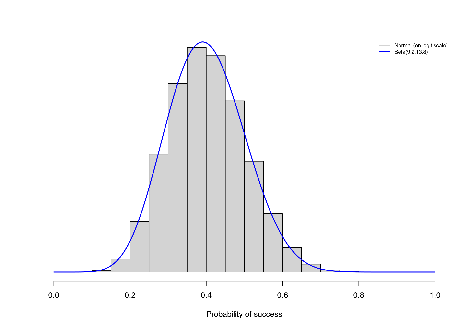
Under the Beta model, it is possible to tweak the values of \(\alpha\) and \(\beta\) so that, say, 95% of the prior distribution for \(\theta\) lies between the two extremes of 0.2 and 0.6. As it turns out, choosing \(\alpha=9.2\) and \(\beta=13.8\) accomplishes this goal. The continuous line in Figure 1.1 shows the resulting Beta prior distribution for \(\theta\). Most of the mass (in fact, exactly 95% of the entire density) lies in the interval \([0.2;0.6]\), as required.
Similarly, we could select values for \(\mu\) and \(\sigma\) to build a Normal distribution that encodes the same information — but notice that \(\mu\) and \(\sigma\) are defined on a different scale, so care would be needed to identify the correct values. For example, if we used \(\mu=\mbox{logit}(0.4)=-0.41\) and \(\sigma=0.413\)3, this would induce a prior distribution on \(\phi\) that effectively represents the same information on the natural scale of \(\theta\).
The histogram in Figure 1.1 depicts the logit-Normal prior on \(\theta\) (\(i.e.\) the rescaled version of the Normal prior distribution on \(\phi\)) — as it is possible to see, this is virtually identical with the Beta prior described above.
1.2.2.3 Model the relevant parameters
In other circumstances, it is more difficult to give the parameters a physical meaning and thus defining a “good” prior distribution requires a bit more ingenuity. For example, costs are usually characterised by a markedly skewed distribution and thus a suitable model is the Gamma, which is characterised by two parameters \(\pmb\theta=(\eta,\lambda)\). These represent, respectively, the shape and the rate.
The difficulty with this distribution is that the “original-scale” parameters are quite hard to interpret in a physical sense; in fact, they are just a mathematical construction that defines the probability density, which happens to be reasonable for a variable such as the costs associated with an intervention. It is more difficult in this case to give a clear meaning to the parameters and thus eliciting a suitable prior distribution (possibly encoding some substantive knowledge) becomes more complicated (Baio, 2013).
It is in general much easier to think in terms of some “natural-scale” parameters, say \(\pmb\omega=(\mu,\sigma)\), representing for example the mean and standard deviation of the costs on the natural scale. This is because we have a better grasp of what these parameters mean in the real world and thus it is possible for us to figure out what features we should include in the model that we choose. In addition to this, as we briefly mentioned in Section 1.1 and will reprise in Section 1.3 and in Section 3.3, decision-making is effectively based on the evaluation of the population average values for the economic outcomes and thus the mean of the cost distribution is in fact the parameter of direct interest.
Typically, there is a unique deterministic relationship \(\pmb\omega=h(\pmb\theta)\) linking the natural- to the original-scale parameters which define the mathematical form of the distribution. As we hinted above, defining a prior on \(\pmb\omega\) will automatically imply one for \(\pmb\theta\). For example, by the mathematical properties of the Gamma density, the elements of \(\pmb\omega\) (on which we want to set the priors) are defined in terms of the elements of \(\pmb\theta\) as \[ \mu = \frac{\eta}{\lambda} \qquad \mbox{and} \qquad \sigma = \sqrt{\frac{\eta}{\lambda^2}} \tag{1.3}\]
(similar relationships are in general available for the vast majority of probability distributions). Whatever the choice for the priors on the natural-scale parameters, in the case of the Gamma distribution, inverting the deterministic relationships in Equation 1.3 it is easy to obtain \[ \eta = \mu \lambda \qquad \mbox{and} \qquad \lambda = \frac{\mu}{\sigma^2}. \tag{1.4}\]
More importantly, because \(\mu\) and \(\sigma\) are random variables associated with a probability distribution, so will be \(\eta\) and \(\lambda\) and thus the prior on \(\pmb\omega\) automatically induces the prior for \(\pmb\theta\).
1.2.2.4 How much information should be included in the prior?
Undoubtedly, the level of information contained in the prior plays a crucial role in a Bayesian analysis, since its influence on the posterior and predictive distributions may be large. This is particularly relevant in cases where the evidence provided by the data is weak (for instance in the case of very small sample sizes). In these situations, it is advisable to use as much information as possible in the prior, to complement the limited amount of information present in the observed data and to perform substantial sensitivity analysis to identify crucial assumptions that may bias the analysis.
On the other hand, in cases where a large amount of data is available to directly inform a parameter, then the prior distribution becomes, to some extent, less influential. In such a situation, it is perhaps reasonable, or at least less critical, to encode a lower level of information in the prior. This can be achieved for example by using Uniform priors on a suitable range, or Normal priors centered on 0 and with very large variances. These “vague” (also referred to as “minimally informative” or “flat”) priors can be used to perform an analysis in which the data drive the posterior and predictive results.
We note, however, that the choice of vague prior depends on the nature and physical properties of the parameters; for example, variances need to be defined on a positive range \((0; +\infty)\) and thus it is not sensible to use a flat Normal prior (which by definition extends from \(-\infty\) to \(+\infty\)). Perhaps, a reasonable alternative would be to model some suitable transformation of a variance (\(e.g.\) its logarithm) using a Normal vague prior — but of course, care is needed in identifying the implications of this choice on the natural scale (we return to this point in the next section).
There is then a sense in which, even when using minimally informative priors, some substantial information is included in the modelling. Consequently, in any case the general advice is that, when genuine information is available, it should be included in the model in a clear and explicit way and that sensitivity analysis should be thoroughly performed.
This aspect is well established in health economic evaluation, particularly under the Bayesian approach. For instance, back to the simple cost example, one possibility is to model the priors on \(\pmb \omega\) using vague Uniform distributions: \[ \mu \sim \mbox{Uniform}(0,H_\mu)\quad \mbox{and} \quad \sigma \sim \mbox{Uniform}(0,H_\sigma), \]
for suitably selected values \(H_\mu,H_\sigma\). This would amount to assuming that values in \([0;H_\mu]\) are all reasonable for the population average cost of the treatment under study — and a similar reasoning would apply to the standard deviation. Of course, this may not be the best choice and were genuine information available, we should include it in the model. For example, the nature of the intervention is clearly known to the investigator and thus it is plausible that some “most-likely range” be available at least approximately.
1.2.2.5 Assess the implications of the assumptions
In addition to performing sensitivity analysis to assess the robustness of the assumptions, in a Bayesian context it is important to check the consistency of what the priors imply. For instance, in the cost model we may choose to use a vague specification for the priors of the natural-scale parameters. Nevertheless, the implied priors for the original-scale parameters will in general not be vague at all. In fact by assuming a flat prior on the natural-scale parameters, we are implying some information on the original-scale parameters of the assumed Gamma distribution.
One added advantage of modelling directly the relevant parameters is that this is not really a problem; the resulting posterior distributions will be of course affected by the assumptions we make in the priors; but, by definition, however informative the implied priors for \((\eta,\lambda)\) turn out to be, this will by necessity be consistent with the substantive knowledge (or lack thereof) that we are assuming for the natural-scale parameters.
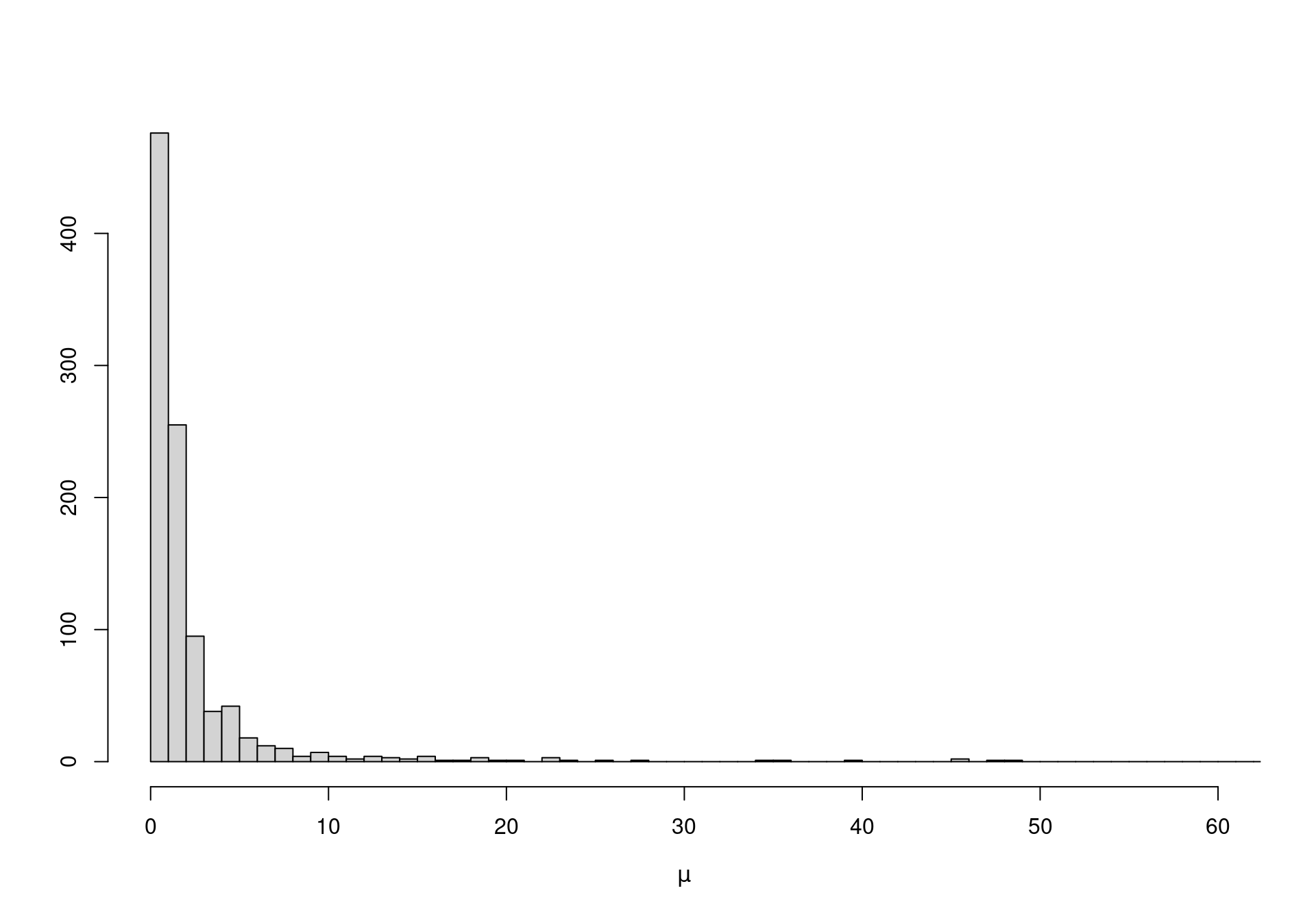
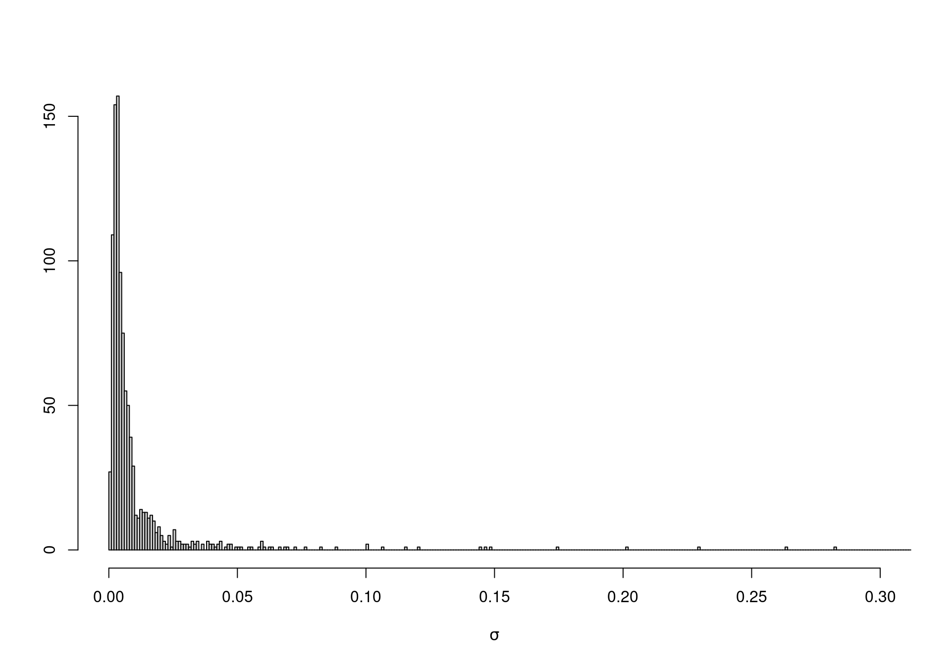
On the other hand, when vague priors are used for original-scale parameters (which may not be the focus of our analysis), the unintended information may lead to severe bias in the analysis. For instance, suppose we model directly \(\eta \sim \mbox{Uniform}(0,10000)\) and \(\lambda \sim \mbox{Uniform}(0,10000)\), with the intention of using a vague specification. In fact, using Equation 1.4 we can compute the implied priors for \(\mu\) and \(\sigma\). Figure 1.2 shows how both these distributions place most of the mass to very small values — possibly an unreasonable and unwanted restriction.
1.2.2.6 Computational issues
While in principle Bayesian analysis may be arguably considered conceptually straightforward, the computational details are in general not trivial and make it generally complex. Nevertheless, under specific circumstances (and for relatively simple models), it is possible to obtain analytic solutions to the computation of posterior and predictive distributions.
One such case involves the use of conjugate priors (Raiffa and Schlaifer, 1961). These indicate a particular mathematical formulation where the prior is selected in a way that, when combined with the model chosen for the data, the resulting posterior is of the same form. For example, if the available data \(y\) are binary and are modelled using a Bernoulli distribution \(y \sim \mbox{Bernoulli}(\theta)\) or equivalently \(p(y\mid\theta)=\theta^y(1-\theta)^{(1-y)}\), it can be easily proven4 that choosing a Beta prior \(\theta \sim \mbox{Beta}(\alpha,\beta)\) yields a posterior distribution \(\theta\mid y \sim \mbox{Beta}(\alpha^*,\beta^*)\), with \(\alpha^*=\alpha+y\) and \(\beta^*=\beta+1-y\). In other words, updating from the prior to the posterior occurs within the same probability family (in this case the Beta distribution) — in effect, the information provided by the data is entirely encoded in the updated parameters \((\alpha^*,\beta^*)\).
The obvious implication is that no complex mathematical procedure is required to compute the posterior (and, similarly, the predictive) distribution. This is a very appealing way of setting up a Bayesian model, mainly because several standard conjugated models exist — see for example Baio (2012). In addition, it is often easy to encode prior information using conjugate models — one simple example of a conjugate, informative prior was given above, when constructing the Beta distribution shown in Figure 1.1).
On the other hand, conjugate priors are dictated purely by mathematical convenience and they fail to fully allow the inclusion of genuine or substantial knowledge about the nature of the model and its parameter. For this reason, in all but trivial cases, conjugate priors become a limitation rather than an asset to a Bayesian analysis; for example, no conjugate prior exist for the popular logistic regression model.
Thus, it is usually necessary to go beyond conjugacy and consider more complex priors. This, however, comes at the price of increased computation complexity and often no analytic or closed form solution exists for the posterior or the predictive distribution. In these cases, inference by simulation is usually the preferred solution.
1.2.3 Bayesian computation
Arguably, the main reason for the enormous increase in the use of the Bayesian approach in practical applications is the development of simulation algorithms and specific software that, coupled with the availability of cheap computational power (which become widespread in the 1990s), allow the end-user to effectively use suitable analytic models, with virtually no limitation in terms of the complexity.
The main simulation method for Bayesian inference is Markov Chain Monte Carlo (MCMC), a class of algorithms for sampling from generic probability distributions — again, we do not deal here with technicalities, but refer the readers to Gilks et al. (1996); Gamerman (1997); Robert and Casella (2004); Gelman et al. (2004); Jackman (2009); Carlin and Louis (2009); Robert and Casella (2010); Brooks et al. (2011). Robert and Casella (2011) review the history and assess the impact of MCMC. Spiegelhalter et al. (2004) discuss the application of MCMC methods to clinical trials and epidemiological analysis, while Baio (2012) and Welton et al. (2012) present the main feature of MCMC methods and their applications, specifically to the problem of health economic evaluation.
In a nutshell, the idea underlying MCMC is to construct a Markov chain, a sequence of random variables for which the distribution of the next value only depends on the current one, rather than the entire history. Given some initial values, this process can be used to repeatedly sample and eventually converge to the target distribution, \(e.g.\) the posterior distribution for a set of parameters of interest. Once convergence has been reached, it is possible to use the simulated values to compute summary statistics (\(e.g.\) mean, standard deviation or quantiles), or draw histograms to characterise the shape of the posterior distributions of interest.
Figure 1.3 depicts the MCMC procedure for the case of two parameters \((\mu,\sigma)\); in this case, we superimpose the “true” joint density (the solid dark ellipses), which is the “target” for the simulation algorithm. Obviously, this is done for demonstration only — in general we do not know what the target distribution is (and this is why we use MCMC to estimate it!).
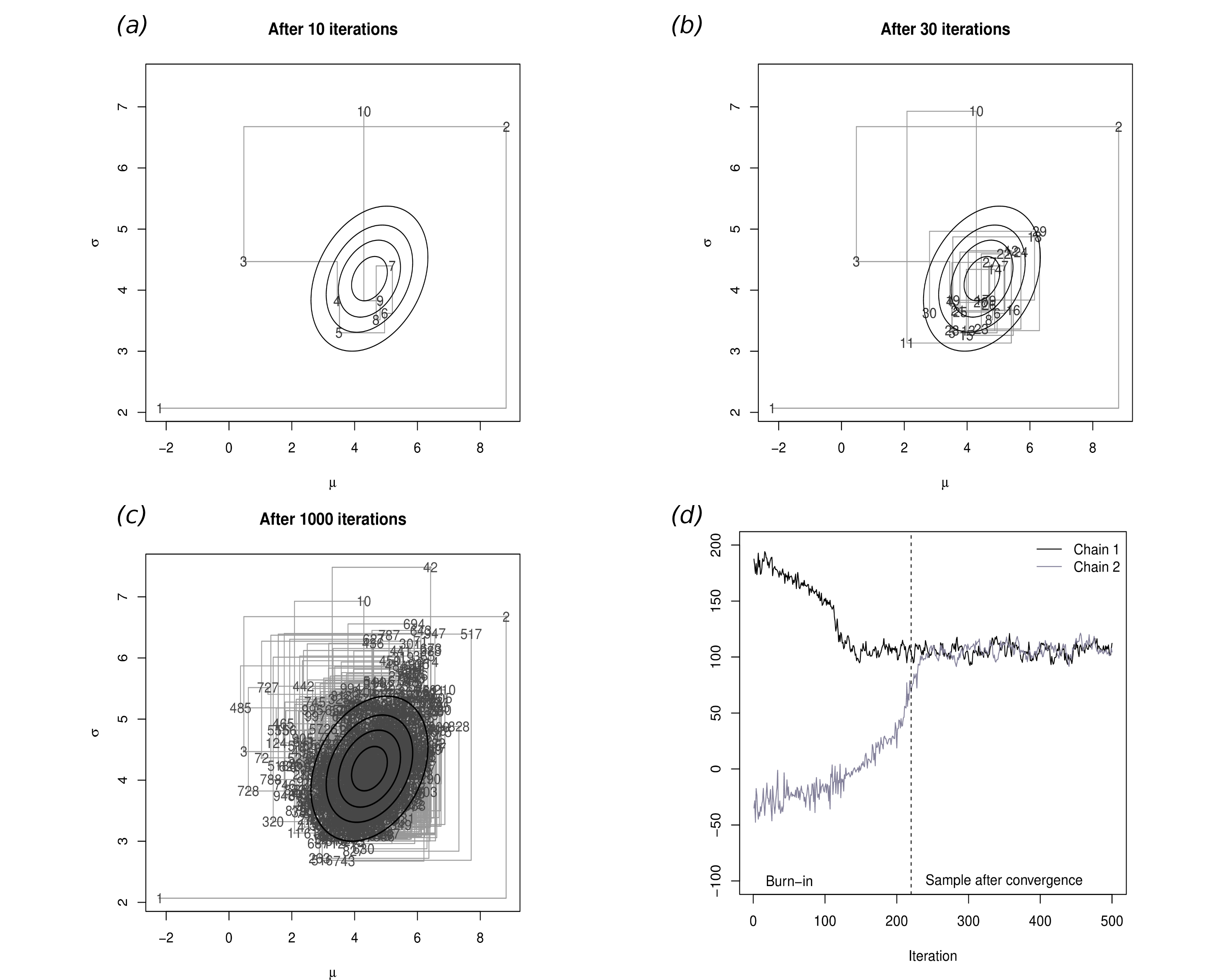
Panel (a) shows the first 10 iterations of the process: the first iteration (labelled as 1) is set as the initial value and it happens to be in a part of the relevant space that is not covered by the “true” distribution. Thus, this point is really not representative of the underlying target distribution. In fact, as is common, the first few values of the simulation are spread all over the space and do not really cover the target area.
However, as the number of simulations increases in panel (b), more and more simulated points actually fall within the “true” distribution, because the process is reaching convergence. In panel (c), after 1000 iterations effectively all of the target area has been covered by simulated values, which can be then used to characterise the joint posterior distribution \(p(\mu,\sigma)\).
It is interesting to notice that, in general, it is possible to construct a suitable Markov chain for a very wide range of problems and, more importantly, given a sufficient number of simulations, it can be proved that it is almost certain that the Markov chain will in fact converge to the target (posterior) distribution. However, this process may require a large number of iterations before it actually starts visiting the target area, rather than points in the parametric space that have virtually no mass under the posterior distribution (\(e.g.\) the points labelled as 1,2,3,10 and 11 in Figure 1.3. For this reason it is essential to carefully check convergence and typically to discard the iterations before convergence.
Panel (d) shows a traceplot for two parallel Markov chains, which are initialised in different values: this graph plots on the \(x-\)axis the number of simulations performed and on the \(y-\)axis the simulated values. As the number of simulations increases, the two chains converge to a common area and mix up. We can visually inspect graphs such as this and determine the point at which convergence has occurred. All the simulations preceding this point are then discarded, while those after convergence are used to perform the analysis.
For example, consider the simple case where there is only one scalar parameter of interest. After the model is successfully run, we can typically access a vector of \(n_{sim}\) simulations \(\pmb{\tilde\theta} = (\tilde\theta_1,\ldots,\tilde\theta_{n_{\text{sim}})}\) from the posterior. We can use this to summarise the results, for example by computing the posterior mean \[ \mathbb{E}[\theta \mid y] = \frac{1}{n_{\text{sim}}} \sum_{i=1}^{n_{\text{sim}}} \tilde \theta_i, \]
or identifying suitable quantiles (for example the 2.5% and 97.5%), to give an approximate (in this case 95%) credible interval.
If the MCMC algorithm has run successfully5, then the information provided in \(\pmb{\tilde\theta}\) will be good enough to fully characterise the variability in the posterior distribution. Of course, ideally we would like to use a large enough number of simulations; often, \(n_{\text{sim}}\) is set to 1000, although this is pretty much an arbitrary choice. Depending on the underlying variability in the target distribution, this number may not be sufficient to fully characterise the entire distribution (although it will usually estimate with suitable precision its core). Again, we refer to, for instance, Baio (2012) for more details. Examples of the procedure described above are also presented in Section 2.3.1 and Section 2.4.1.
1.3 Basics of health economic evaluation
Health economics is typically concerned with evaluating a set of interventions \(t\in\mathcal{T}=(0,1,\ldots,T)\) that are available to treat a given condition. These may be drugs, life-style modification or complex interventions — the general concepts of economic evaluations apply regardless. We only consider here the most important issues; comprehensive references include Willan and Briggs (2006); Briggs et al. (2006); Baio (2012).
As mentioned above, the economic outcome is a multivariate response \(y=(e,c)\), represented by a suitable clinical outcome (\(e.g.\) blood pressure or occurrence of myocardial infarction), together with a measure of the costs associated with the given intervention. On the basis of the available evidence (\(e.g.\) coming from a randomised controlled trial or a combination of different sources, including observational data), the problem is to decide which option is “optimal” and should then be applied to the whole homogenous population. In the context of publicly funded health-care systems (such as those in many European countries, including the UK National Health Service, NHS), this is a fundamental problem as public resources are finite and limited and thus it is often necessary to prioritise the allocation of public funds on health interventions.
Crucially, “optimality” can be determined by framing the problem in decision-theoretic terms (Baio, 2012; Briggs et al., 2006; O’Hagan and Stevens, 2001; Spiegelhalter et al., 2004), which implies the following steps.
- Characterise the variability in the economic outcome \((e,c)\), which is typically due to sampling, using a probability distribution \(p(e,c\mid\pmb\theta)\), indexed by a set of parameters \(\pmb\theta\). Within the Bayesian framework, uncertainty in the parameters is also modelled using a probability distribution \(p(\pmb\theta)\).
- Value the consequences of applying a treatment \(t\), through the realisation of the outcome \((e,c)\) by means of a utility function \(u(e,c;t)\).
- Assess “optimality” by computing for each intervention the expectation of the utility function, with respect to both “population” (parameters) and “individual” (sampling) uncertainty/variability \[\mathcal{U}^t = \mathbb{E}\left[u(e,c;t)\right].\] In line with the precepts of (Bayesian) decision theory, given current evidence the “best” intervention is the one associated with the maximum expected utility. This is because it can be easily proved that maximising the expected utility is equivalent to maximising the probability of obtaining the outcome associated with the highest (subjective) value for the decision-maker (Baio, 2012; Bernardo and Smith, 1999; Briggs et al., 2006; Lindley, 2006).
Under the Bayesian framework, \(\mathcal{U}^t\) is dimensionless, \(i.e.\) it is a pure number, since both sources of basic uncertainty have been marginalised out in computing the expectation. Consequently, the expected utility allows a direct comparison of the alternative options.
While the general setting is fairly straightforward, in practice, the application of the decision-theoretic framework for health economic evaluation is characterised by the following complications.
- As any Bayesian analysis, the definition of a suitable probabilistic description of the current level of knowledge in the population parameters may be difficult and potentially based on subjective judgement.
- There is no unique specification of the method of valuation for the consequences of the interventions is (\(i.e.\) what utility function should be chosen):
- Typically, replacing one intervention with a new alternative is associated with some risks such as the irreversibility of investments (Claxton, 1999). Thus, basing a decision on current knowledge may not be ideal, if the available evidence-base is not particularly strong/definitive (we elaborate on this point in Chapter 4).
As for the utility function, health economic evaluations are generally based on the (monetary) net benefit (Stinnett and Mullahy, 1998) \[ u(e,c;t) = ke - c. \tag{1.5}\]
Here \(k\) is a willingness-to-pay parameter, used to put cost and benefits on the same scale and represents the budget that the decision-maker is willing to invest to increase the benefits by one unit. The main appeal of the net benefit is that it has a fixed form, once the variables \((e,c)\) are defined, thus providing easy guidance to valuation of the interventions. Moreover, the net benefit is linear in \((e,c)\), which facilitates interpretation and calculations. Nevertheless, the use of the net benefit presupposes that the decision-maker is risk neutral, which is by no means always appropriate in health policy problems (Koerkamp et al., 2007).
If we consider the simpler scenario where \(\mathcal{T}=(1,2)\), where \(t=1\) is some sort of “status quo” and \(t=2\) is the new treatment whose cost-effectiveness is being assessed, decision-making can be equivalently effected by considering the expected incremental benefit (of treatment \(2\) over treatment \(1\)) \[ \mbox{EIB} = \mathcal{U}^2 - \mathcal{U}^1 \tag{1.6}\]
- of course, if \(\mbox{EIB}>0\), then \(\mathcal{U}^2 > \mathcal{U}^1\) and therefore \(t=2\) is the optimal treatment (being associated with the highest expected utility).
In particular, using the monetary net benefit as utility function, Equation 1.6 can be re-expressed as \[ \mbox{EIB} = \mathbb{E}[k\Delta_e - \Delta_c] = k\mathbb{E}[\Delta_e] - \mathbb{E}[\Delta_c] \tag{1.7}\] where \[ \Delta_e = \mathbb{E}[e\mid \pmb\theta^2] - \mathbb{E}[e\mid\pmb\theta^1] = \mu^2_e -\mu^1_e \] is the average increment in the benefits (from using \(t=2\) instead of \(t=1\)) and similarly \[ \Delta_c = \mathbb{E}[c \mid \pmb \theta^2] - \mathbb{E}[c \mid \pmb \theta^1] = \mu^2_c - \mu^1_c \] is the average increment in costs deriving from selecting \(t=2\).
If we define the Incremental Cost-Effectiveness Ratio as \[ \mbox{ICER} = \frac{\mathbb{E}[\Delta_c]}{\mathbb{E}[\Delta_e]} \] then it is straightforward to see that when the net monetary benefit is used as utility function, then \[ \mbox{EIB} >0 \quad \mbox{if and only if} \quad \left\{ \begin{array}{lr} \displaystyle k>\frac{\mathbb{E}[\Delta_c]}{\mathbb{E}[\Delta_e]}=\mbox{ICER}, & \quad \mbox{for }\mathbb{E}[\Delta_e]>0 \\[10pt] \displaystyle k<\frac{\mathbb{E}[\Delta_c]}{\mathbb{E}[\Delta_e]}=\mbox{ICER}, & \quad \mbox{for }\mathbb{E}[\Delta_e]<0 \end{array} \right. \] and thus decision-making can be equivalently effected by comparing the ICER to the willingness-to-pay threshold.
Notice that, in the Bayesian framework, \((\Delta_e,\Delta_c)\) are random variables, because while sampling variability is being averaged out, these are defined as functions of the parameters \(\pmb\theta=(\pmb\theta^1,\pmb\theta^0)\). The second layer of uncertainty (\(i.e.\) the population, parameters domain) can be further averaged out. Consequently, \(\mathbb{E}[\Delta_e]\) and \(\mathbb{E}[\Delta_c]\) are actually pure numbers and so is the ICER.
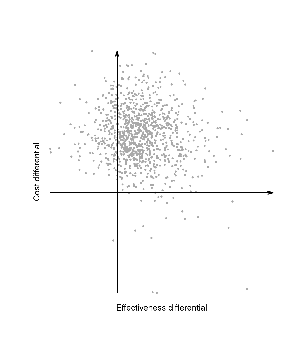
The two layers of uncertainty underlying the Bayesian decision-making process as well as the relationships between the variables defined above can be best appreciated through the inspection of the cost-effectiveness plane, depicting the joint distribution of the random variables \((\Delta_e,\Delta_c)\) in the \(x-\) and \(y-\)axis, respectively.
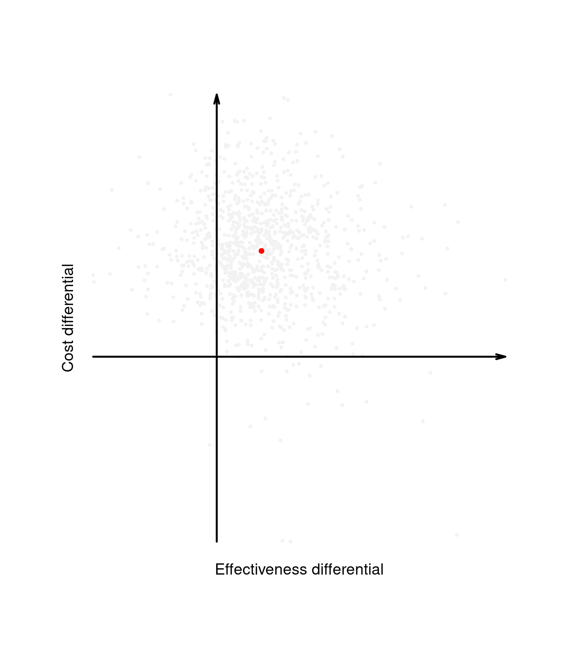
Intuitively, the cost-effectiveness plane characterises the uncertainty in the parameters \(\pmb\theta\). This is represented by the dots populating the graph in Figure 1.4 (a), which can be obtained, for example, by simulation. By taking the expectations over the marginal distributions for \(\Delta_e\) and \(\Delta_c\), we then marginalise out this uncertainty and obtain a single point in the plane, which represents the “typical future consequence”. This is shown as the dot in Figure 1.4 (b), where the underlying distribution has been shaded out.
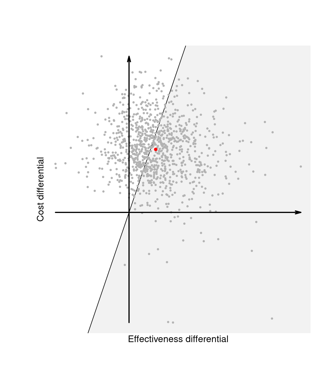
Figure 1.4 (c) also shows the “sustainability area”, \(i.e.\) the part of the cost-effectiveness plane which lies below the line \(\mathbb{E}[\Delta_c] = k\mathbb{E}[\Delta_e]\), for a given value of the willingness-to-pay \(k\). Given the equivalence between the EIB and the ICER, interventions for which the ICER is in the sustainability area are more cost-effective than the comparator. Changing the value for the threshold, may modify the decision as to whether \(t=2\) is the most cost-effective intervention. The EIB can be plot as a function of \(k\) to identify the “break-even point”, \(i.e.\) the value of the willingness-to-pay in correspondence of which the EIB becomes positive.
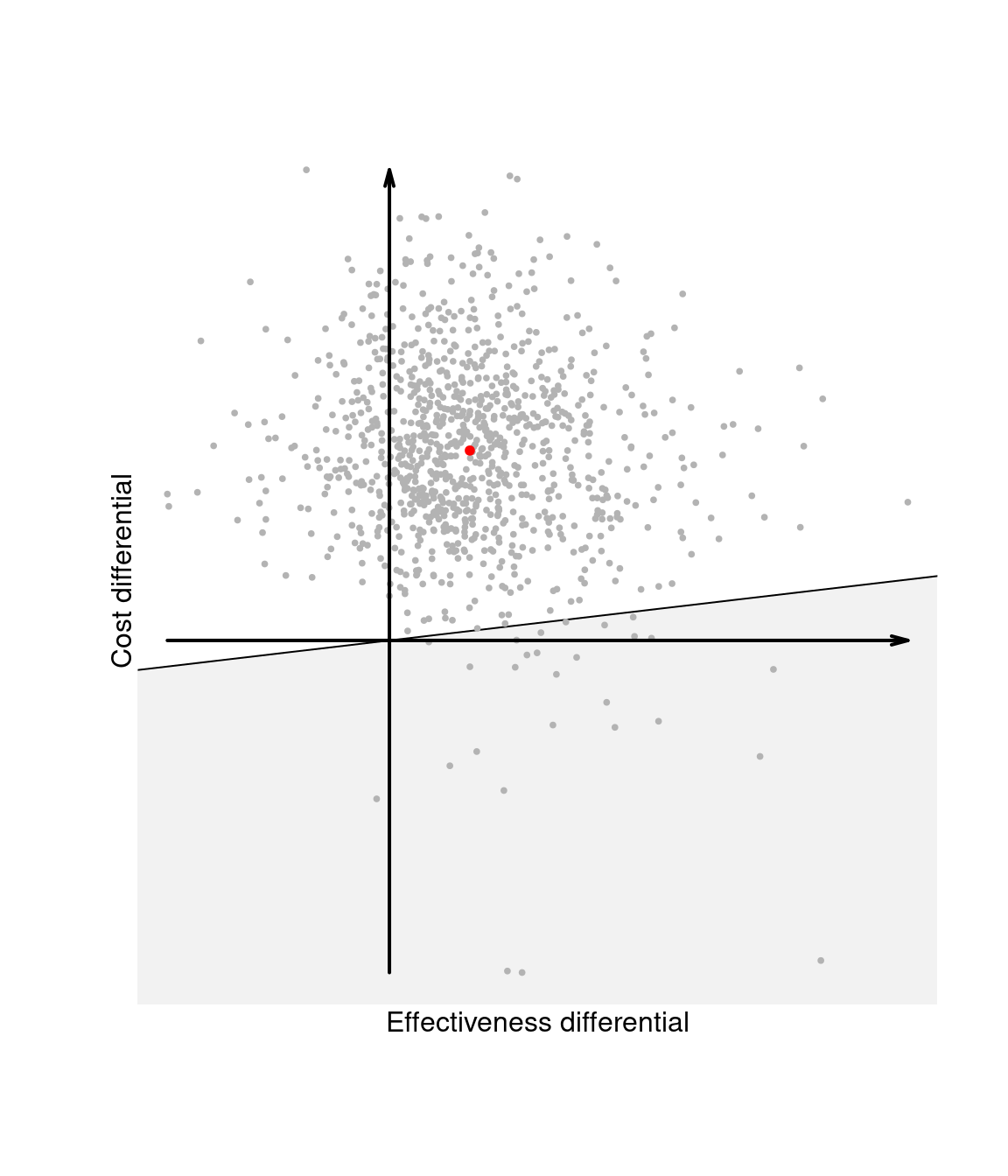
Finally, Figure 1.4 (d) shows the sustainability area for a different choice of the parameter \(k\). In this case, because the ICER — and, for that matter, most of the entire distribution of \((\Delta_e,\Delta_c)\) — lie outside the sustainability area, the new intervention \(t=2\) is not cost-effective. We elaborate this further in Chapter 4, when discussing probabilistic sensitivity analysis.
1.4 Doing Bayesian analysis and health economic evaluation in R
The general process of doing a Bayesian analysis (with a view of using the results of the model to perform an economic evaluation) can be classified according to several steps. We review these steps in the following, relating the process to its practical features and assuming R as the software of choice.
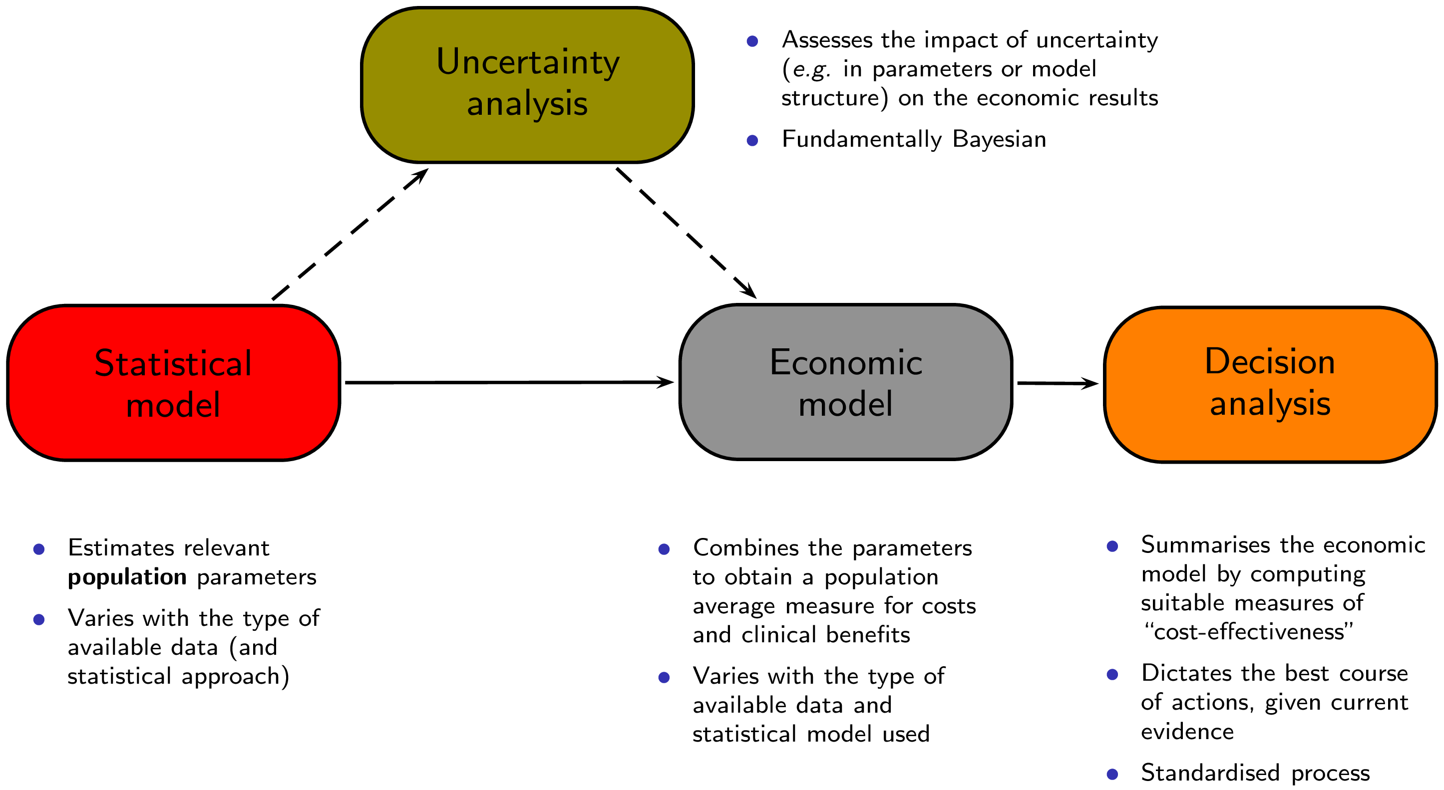
Figure 1.5 shows a graphical representation of this process. The process starts with a statistical model that is used to estimate some relevant parameters, which are then fed to an economic model with the objective of obtaining the relevant population summaries indicating the incremental benefits and costs for a given intervention. These are in turn used as the basis for the decision analysis, as described above. The final aspect is represented by the evaluation of how the uncertainty that characterises the model impacts the final decision-making process. We describe the several steps (building blocks) and their relevance to the analysis in the following.
1.4.1 Pre-processing the data
In this step, we typically create, aggregate and modify the original variables available in the dataset(s) that we wish to analyse. In the context of economic evaluation this may be needed because the outcomes of interest may have to be computed as functions of other observable variables — for example, total costs could be obtained as the sum of several cost items (\(e.g.\) service provision, acquisition of the intervention, additional treatments and so on).
In any case, this step, typically performed directly in R, serves to generate a data list that contains the values of all the variables that are of interest and should be modelled formally. The complexity of this data list depends on the nature of the original data: for example, when dealing with experimental evidence (\(e.g.\) coming from a RCT), often we model directly the quantities of interest (\(i.e.\) the variables of costs and clinical effectiveness or utility).
For example, in the context of an RCT, we would be likely to directly observe the variables \((e_{it},c_{it})\) for individuals \(i=1,\ldots,n_t\) in each treatment arm \(t=1,\ldots,T\) and could model them so that the relevant parameters are their population averages \((\mu_{et},\mu_{ct})\) — see for instance Chapter 4 in Baio (2012).
In other cases, for example when using aggregated data, it is necessary to build a more complex model that directly considers ancillary variables (which may be observed) and these are then manipulated to derive the relevant economic outcomes. This type of modelling is often referred to as “decision-analytic” and it typically amounts to creating a set of relationships among a set of random quantities. A decision tree may be used to combine measures of costs and effectiveness (\(e.g.\) in terms of reduction in the occurrence of adverse events) — examples of this strategy are in Chapter 5 in Baio (2012). We also consider models of this kind in Chapter 2 and in Section 4.4.3.1.
1.4.2 Building and coding the analysis model
This is the most mathematical and in many ways creative part of the process; according to the nature and availability of the data, we need to create a suitable probabilistic model to describe uncertainty. Technically, this step is required even outside of the Bayesian framework that we adopt. Of course, under the Bayesian paradigm, all the principles described in Section 1.2.2 should be applied. Again, depending on the nature of the data, the model may be more or less complex and encode a larger or smaller number of assumptions / probabilistic features.
Assuming that the method of inference is some sort of simulation-based procedure such as MCMC, this step is usually performed by first “translating” the model on a text file, which contains the description of the assumptions in terms of distributional and deterministic relationships among the variables. A “frequentist counterpart” to this step would be the creation of a script which codes the modelling assumptions.
We provide examples of this process under a full Bayesian framework in Chapter 2, where we also briefly discuss the issues related with convergence and model checking.
1.4.3 Running the model
At this point, we can “run the model”, which provides us with an estimation of the quantities of interest. As we have repeatedly mentioned, these may be directly the average costs and benefits under different interventions, or perhaps some other quantities (\(e.g.\) the transition probabilities in a Markov model setting).
In our ideal Bayesian process, this step is performed by specialised software (\(e.g.\) JAGS or BUGS) to run the MCMC procedure, which we typically interface with R. In other words, after we have created the data list and the text file with the model assumptions, we call the MCMC sampler directly from R. This will then take over and run the actual analysis, at the end of which the results will be automatically exported in the R workspace, in the form a suitable object, containing \(e.g.\) the samples from the posterior or predictive distributions of interest. We show in Chapter 2 some examples of this procedure.
Once the model has run, the next step involves checking its performance (\(e.g.\) in terms of convergence, if the procedure is based, as it often is, on an MCMC algorithm). There are several diagnostic tools for MCMC, most of which can be implemented directly in R. Thus, again following our ideal process, at this point the used will have re-gained control of the R session in which the simulations from the model are stored. Standard methods of analysis of convergence and autocorrelation are described in details in many specific text, for instance Gamerman (1997); Gelman et al. (2013); Baio (2012).
The combination of the steps described so far can be thought of as the Statistical model box of Figure 1.5.
1.4.4 Post-processing the results
Perhaps even more importantly, from the health economic point of view, depending on the type of data available, the results of the model may not directly provide the information or variables needed to perform the cost-effectiveness analysis. For instance, while individual level data may be used to estimate directly the average cost and benefits, using aggregated data may mean that the model is estimating some parameters which are not necessarily the actual measures of clinical benefit and cost \((e,c)\).
Thus, it will be often necessary to combine the quantities estimated from the model using logical relationships that define \((e,c)\). For example, the model may estimate the posterior distribution for \(\lambda_t\) and \(\gamma\), indicating respectively the treatment-specific length of hospitalisation for a given disease and the cost associated with it. Neither of these can be directly used as a measure of cost associated with the treatment being considered, but we may construct a new variable \(c_t = \lambda_t\gamma\) to represent it.
This step is described by the Economic model box in Figure 1.5 and performing it in R can be particularly effective — once the full posterior distributions are available to the R workspace, calculations such as the one showed above are generally trivial.
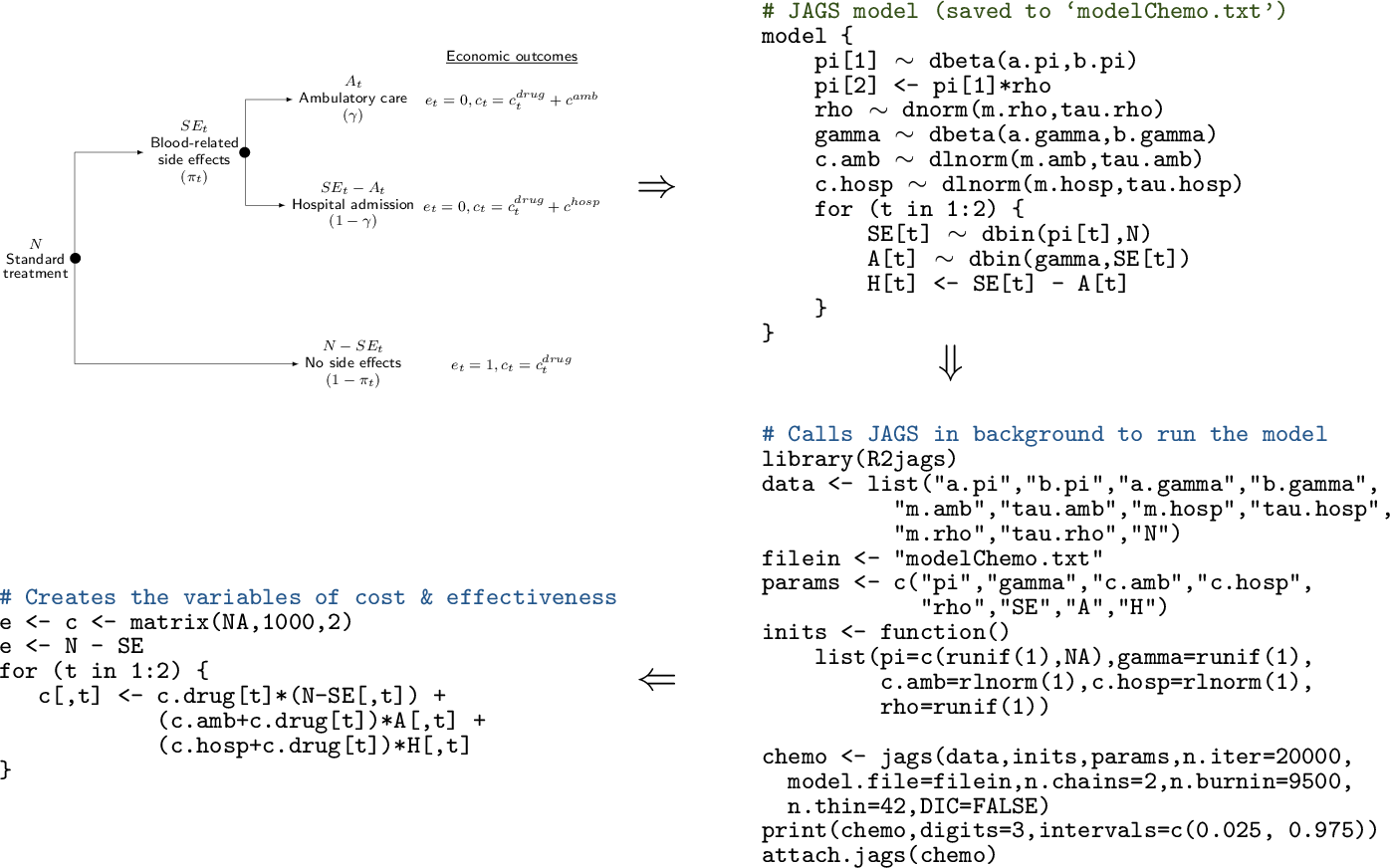
R code to define the data and interface with a specific software (\(e.g.\) JAGS or BUGS). Finally (bottom-left corner), the results of the model are post-processed in R to produce the economic summaries that are then fed to the “Decision analysis” block
Figure 1.6 shows a graphical representation of how the Statistical model and the Economic model described in Figure 1.5 are performed and combined. Basically, the whole process begins with the creation of a model, which describes how the intervention is applied to the relevant population, what the effects are (in terms of benefits and costs) and what variables or parameters are considered. This step may be done in “pen-and-paper” and is in fact the most creative part of the whole exercise. Often, we can rely on simple structures, such as decision trees (as in the top-left corner of Figure 1.6, while sometimes this requires a more complicated description of the underlying reality. Again, notice that this step is required irrespective of the statistical approach considered.
In the full Bayesian framework that we advocate, these assumptions will be translated into code, \(e.g.\) using JAGS or BUGS, as shown in the top-right corner of Figure 1.6; in a non-Bayesian context, other software may be used (\(e.g.\) SAS, Stata or R), but in a sense this procedure of scripting is also common to all statistical approaches and allows to make the model easily replicable. We note here (and return to this point in Section 3.1 that using less sophisticated tools such as Microsoft Excel may render this step less straightforward.
Once the model has been coded up, it can be run to obtain the relevant estimates (bottom-right corner of Figure 1.6. In this case, we consider an R script that defines the data and interfaces with the MCMC software (in this case JAGS) to compute the posterior distributions of the model parameters. Of course, this step needs careful consideration, \(e.g.\) it is important to check model convergence and assess whether the output is reasonable.
Finally (bottom-left corner of Figure 1.6, we can post-process the model output to create the relevant quantities to be passed to the Economic model. In this case, we use again R to combine the model parameters into suitable variables of benefits and costs (e and c, respectively). This step basically amounts to performing the Economic model block of Figure 1.5.
1.4.5 Performing the decision analysis
The rest of the decision process, represented by the Decision analysis box in Figure 1.5, is probably the easiest; in fact, once the relevant quantities have been estimated, the optimal decision given the current knowledge can be derived by computing the summaries described in Section 1.3; the results of this process may be depicted as in panel (b) of Figure 1.4.
The dashed arrows connecting the Statistical model to the Economic model through the Uncertainty analysis box in Figure 1.5 also describe how this process occurs: if the uncertainty described by the posterior distributions is marginalised (averaged) out, then the analysis is performed on the “straight line” from the statistical to the decision analysis. This represents the decision process under current uncertainty and identifies the best course of action today.
On the other hand, if uncertainty is not marginalised, then we can analyse the “potential futures” separately, \(e.g.\) as in panels (a), (c) and (d) of Figure 1.4). A full Bayesian approach will allow to directly perform this form of “probabilistic sensitivity analysis”, which allows the evaluation of the impact of parameters uncertainty on the optimal decision.
1.4.6 Using BCEA
The main objective of this book is to describe how health economic evaluation can be systematised and performed routinely and thoroughly using the R package BCEA — the remaining chapters will present in details the features of the package, using worked examples going through the several steps of the economic analysis.
In a sense, BCEA plays a role in the economic evaluation after the statistical model has been performed. While to use BCEA it is not even strictly necessary to consider a Bayesian approach (we return to this point in Section 3.1 and in Chapter 5, the entire book is based on the premise that the researchers have indeed performed a Bayesian analysis of their clinical and economic data. We stress here however that BCEA only deals with the decision and uncertainty analysis.
References
Baio, G., 2013. Bayesian models for cost-effectiveness analysis in the presence of structural zero costs. Statistics in Medicine 33(11), 1900–1913.
Baio, G., 2012. Bayesian Methods in Health Economics. Chapman Hall/CRC Press, Boca Raton, FL.
Bernardo, J., Smith, A., 1999. Bayesian Theory. John Wiley; Sons, New York, NY.
Briggs, A., Sculpher, M., Claxton, K., 2006. Decision modelling for health economic evaluation. Oxford University Press, Oxford, UK.
Brooks, S., Gelman, A., Jones, G., Meng, X., 2011. Handbook of Markov Chain Monte Carlo. Chapman Hall/CRC, Boca Raton, FL.
Carlin, B., Louis, T., 2009. Bayesian Methods for Data Analysis 3rd edition. Chapman Hall/CRC, Boca Raton, FL.
Christensen, R., Johnson, W., Branscum, A., Hanson, T., 2011. Bayesian Ideas and Data Analyses. Chapman Hall/CRC, Boca Raton, FL.
Claxton, K., 1999. The irrelevance of inference: a decision-making approach to stochastic evaluation of health care technologies. Journal of Health Economics 18, 342–364.
Gamerman, D., 1997. Markov chain monte carlo. Chapman; Hall, London, UK.
Gelman, A., Carlin, J., Stern, H., Dunson, D., Vehtari, A., Rubin, D., 2013. Bayesian Data Analysis - 3rd edition. Chapman Hall/CRC, New York, NY.
Gelman, A., Carlin, J., Stern, H., Rubin, D., 2004. Bayesian Data Analysis - 2nd edition. Chapman Hall, New York, NY.
Gilks, W., Richardson, S., Spiegelhalter, D., 1996. Markov Chain Monte Carlo in Practice. Chapman Hall, London, UK.
Jackman, S., 2009. Bayesian analysis for the social sciences. John Wiley; Sons, New York, NY.
Koerkamp, B., Hunink, M., Stijnen, T., Hammitt, J., Kuntz, K., Weinstein, M., 2007. Limitations of acceptability curves for presenting uncertainty in cost-effectiveness analyses. Medical Decision Making 27 (2), 101–111.
Kruschke, J., 2015. Doing Bayesian Data Analysis: A Tutorial with R and JAGS and Stan, 2nd ed. Academic Press.
Lindley, D., 2006. Understanding uncertainty. John Wiley; Sons, New York, NY.
Lindley, D., 2000. The philosophy of Statistics. The Statistician 49, 293–337.
Lunn, D., Jackson, C., Best, N., Thomas, A., Spiegelhalter, D., 2013. The BUGS book – a practical introduction to Bayesian analysis. Chapman Hall/CRC, New York, NY.
McElreath, R., 2015. Statistical Rethinking: A Bayesian Course with Examples in R and Stan. Chapman; Hall/CRC, Boca Raton, FL.
O’Hagan, A., Stevens, J., 2001. A framework for cost-effectiveness analysis from clinical trial data. Health Economics 10, 303–315.
O’Hagan, A., Stevens, J., Montmartin, J., 2001. Bayesian cost effectiveness analysis from clinical trial data. Statistics in Medicine 20, 733–753.
Raiffa, H., Schlaifer, H., 1961. Applied Statistical Decision Theory. Harvard University Press, Boston, MA.
Robert, C., 2001. The bayesian choice - 2nd edition. Springer Verlag, New York, NY.
Robert, C., Casella, G., 2011. A Short History of Markov Chain Monte Carlo: Subjective Recollections from Incomplete Data. Statistical Science 26, 102–115.
Robert, C., Casella, G., 2010. Introducing monte carlo methods with r. Springer Verlag, New York, NY.
Robert, C., Casella, G., 2004. Monte carlo statistical methods - 2nd edition. Springer Verlag, New York, NY.
Spiegelhalter, D., Abrams, K., Myles, J., 2004. Bayesian Approaches to Clinical Trials and Health-Care Evaluation. John Wiley; Sons, Chichester, UK.
Stinnett, A., Mullahy, J., 1998. Net health benefits: a new framework for the analysis of uncertainty in cost effectiveness analysis. Medical Decision Making 18 (Suppl), S68–S80.
Welton, N.J., Sutton, A.J., Cooper, N.J., Abrams, K.R., Ades, A.E., 2012. Evidence synthesis for decision making in healthcare. John Wiley & Sons, Ltd.
Willan, A., Briggs, A., 2006. The statistical analysis of cost-effectiveness data. John Wiley; Sons, Chichester, UK.
For instance, recall that p-values are defined in terms of the chance of obtaining data that are even more extreme than the one that have actually observed.↩︎
While this discussion is beyond the objectives of this book, we re-iterate here that in a “hard-core” Bayesian approach, parameters are just convenient mathematical abstractions that simplify the modelling for an observable variable \(y\) — see for example Baio (2012) and the references therein.↩︎
We need to encode the assumption that, on the logit scale, 0.6 is the point beyond which only 2.5% of the mass lies. Given the assumption of normality, this is easy to obtain by setting \(\mbox{logit}(0.4)+1.96\sigma=\mbox{logit}(0.6)\) from which we can easily derive \(\sigma = \frac{\mbox{logit}(0.6)-\mbox{logit}(0.4)}{1.96}=0.413\).↩︎
The basic idea is to investigate the form of the likelihood function \(\mathcal{L}(\theta)\), \(i.e.\) the model for the data \(p(y\mid \theta)\), but considered as a function of the parameters. If \(\mathcal{L}(\theta)\) can be written in terms of a known distribution, then this represents the conjugate family. For instance, the Bernoulli likelihood is \(\mathcal{L}(\theta)=p(y\mid\theta)=\theta^y(1-\theta)^{(1-y)}\), which is actually the core of a Beta density. When computing the posterior distribution by applying Bayes theorem and combining the likelihood \(\mathcal{L}(\theta)\) with the conjugate prior, effectively the two terms have the same mathematical form, which leads to a closed form for the posterior.↩︎
All the references cited above discuss at great length the issues of convergence and autocorrelation and methods (both visual and formal) to assess them. In the discussion here, we assume that the actual convergence of the MCMC procedure to the relevant posterior or predictive distributions has been achieved and checked satisfactorily, but again, we refer the reader to the literature mentioned above for further discussion and details. We return to this point in Chapter 2 when describing the case studies.↩︎