| Model | \(\hat{\pi}\) | \(\hat{S}({\mnum{20}})\) |
|---|---|---|
| Weibull MCM | 0% | 0.2% |
| NMCM, 5 years knot | 62% | 19% |
| NMCM, 15 years knot | 49% | 15% |
| Observed | 20.1% (13.5-27.5) |
Mixture Cure Models: Do they create more issues than they are trying to solve?
1. Evolution of MCM modelling
https://gianluca.statistica.it | https://egon.stats.ucl.ac.uk/research/statistics-health-economics
https://github.com/giabaio | https://github.com/StatisticsHealthEconomics
@gianlubaio@mas.to | gianluca-baio
9 November 2026
ISPOR Europe, Vienna
Check out our departmental podcast “Random Talks” on Soundcloud!
Follow our departmental social media accounts + magazine “Sample Space”
Department of Statistical Science | University College London
Extrapolation in HTA: a recipe for disaster
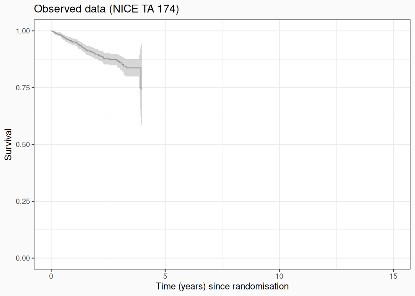
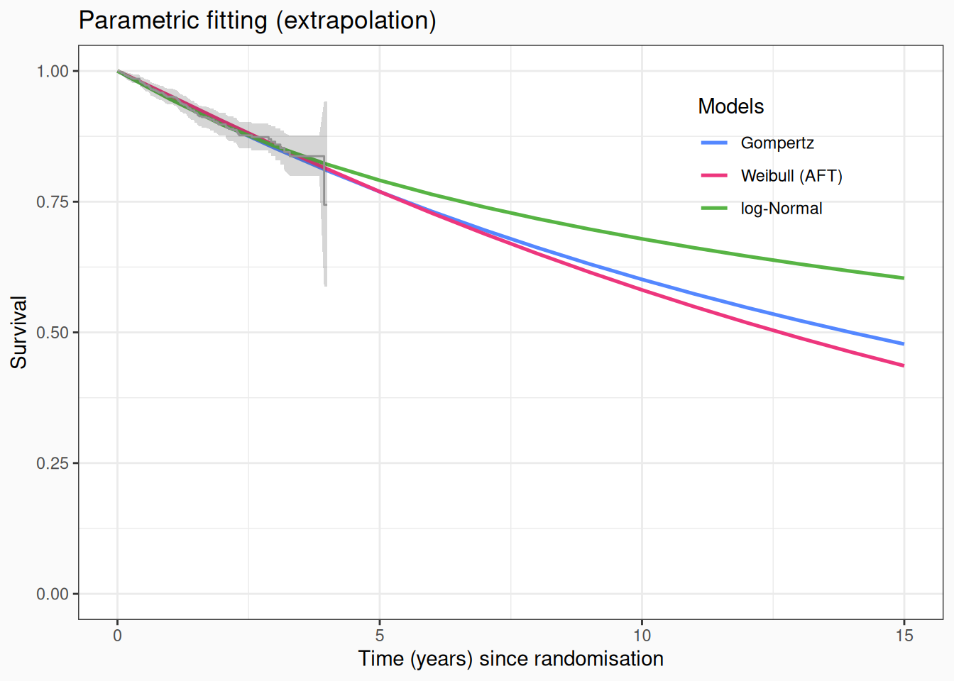
- Intrinsic/pathological uncertainty in the output of the (time-to-event) statistical modelling does carry through the entire process, all the way to the decision-making
- It is not impossible (especially in cases involving new, innovative immuno-oncology drugs) that the observed data be extremely sparse and subject to high censoring
- In the case depicted here, the best fitting model responds by extrapolating a survival curve that implies Pr(alive at 15 years) \(\approx\) 0.5
- This may be obviously wrong/against expert or clinical opinion!
Naïve/vanilla mixture cure model
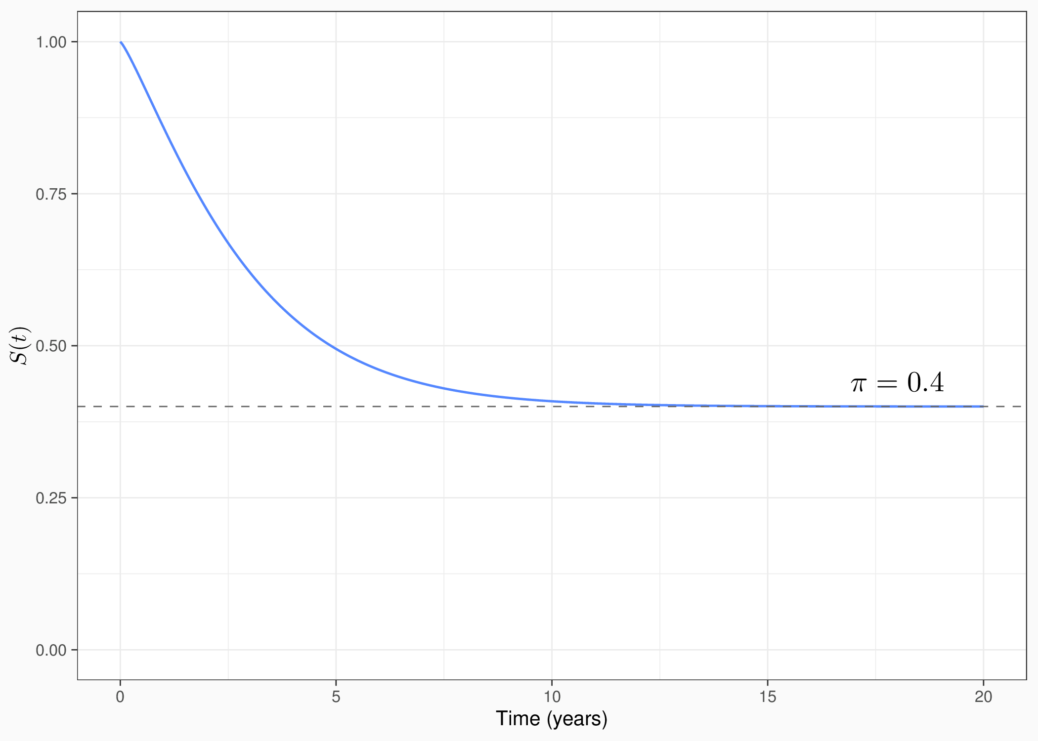
\[ S(t) =\pi + ({\mnum{1}}-\pi)\, S_u(t;\theta) \]
- \(\pi\): “cure fraction” (proportion of “cured” individuals)
- \(S_u\): parametric survival for the “uncured”
- \(S(t) \to \pi\) as \(t \to \infty\): plateau
Two structural issues:
- no direct background mortality in the fit: cured patients live forever
- possible inconsistency across endpoints: PFS (time to progression or death) and OS (time to death) fitted independently
Non-mixture cure model (NMCM)
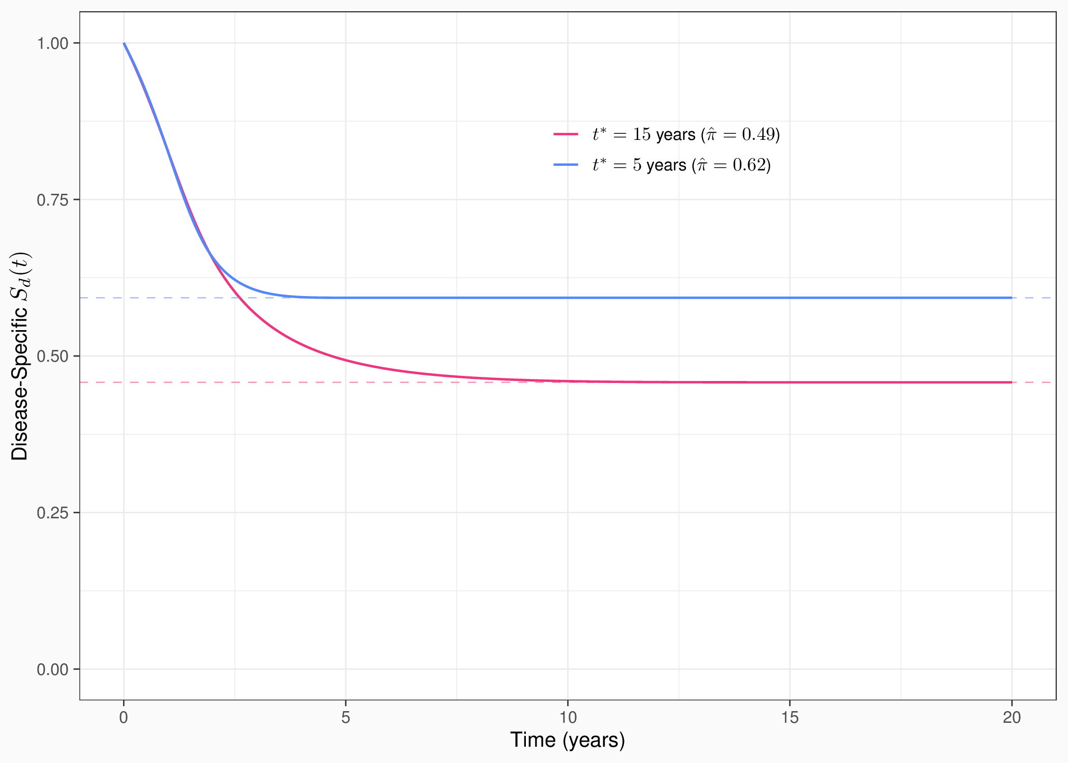
Consider a (re-parameterised) model with disease-specific survival
\[ S_{d}(t) = \pi^{G(t)} = \exp\{-\theta G(t)\}, \qquad \theta = -\log\pi \]
- \(G(t)\) is an auxiliary/latent CDF, governing the pace at which the population moves toward the cure plateau
- \(G(t)\to {\mnum{1}} \Rightarrow S_d(t)\to\pi\)
- Can include background mortality: \(S(t) = S^*(t) S_d(t)\)
- No explicit cured/uncured mixture
- \(S_u\) describes a latent uncured class — hard to pin down without enough follow-up past the plateau
- \(G(t)\) shapes \(S_d(t)\) directly and every observed event contributes to its identification
- The cure fraction emerges from the estimated asymptote of \(S_d(t)\)
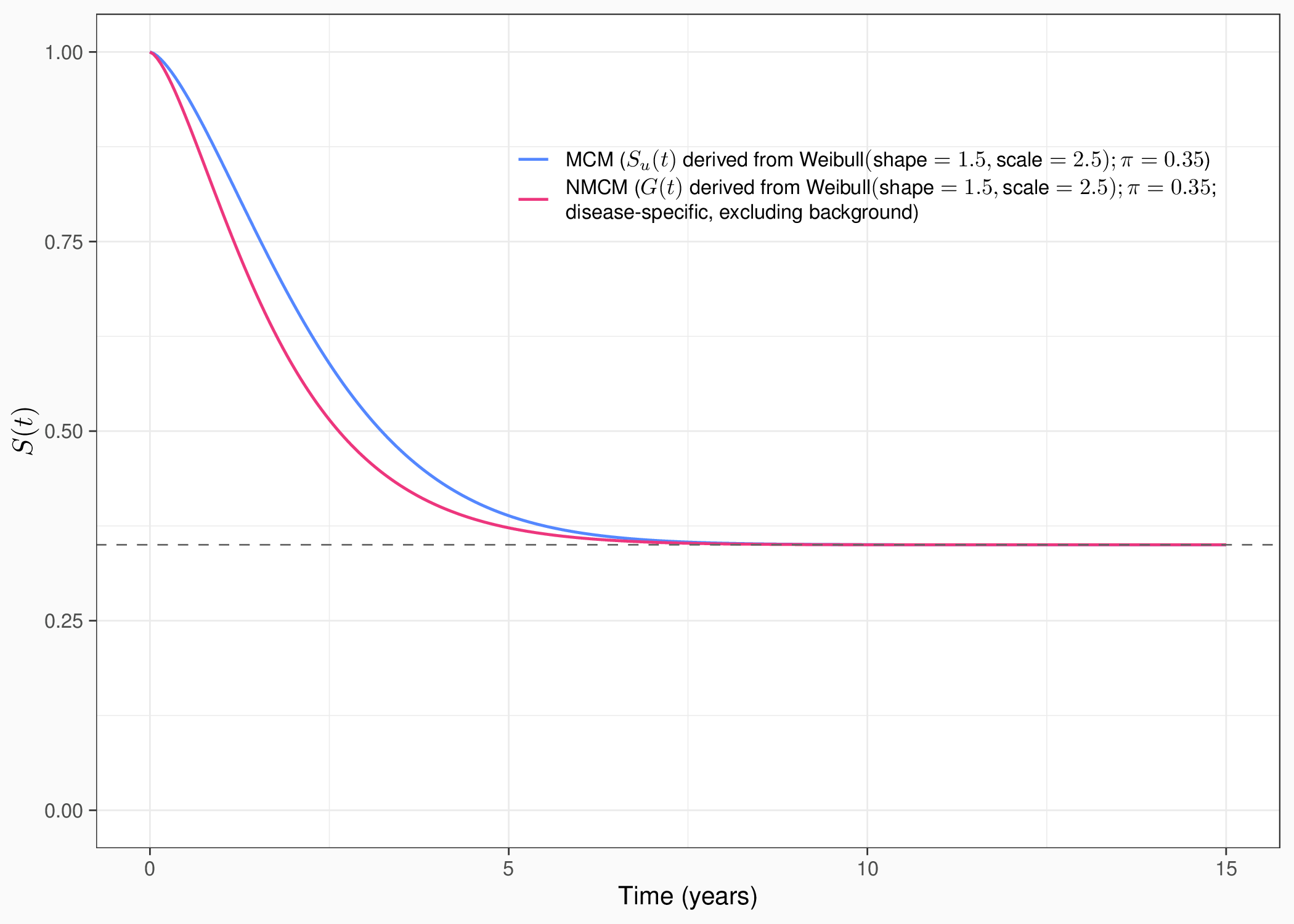
- With the same \(\pi\) fraction and the same underlying parameterisation, the MCM declines more slowly
Software: flexsurv::flexsurvcure(mixture=FALSE)
Latimer NR, Rutherford MJ. (2024) Mixture and Non-mixture Cure Models for Health Technology Assessment: What You Need to Know. PharmacoEconomics, 42(10):1073-1090. doi:10.1007/s40273-024-01406-7
Flexible parametric NMCM
Royston-Parmar splines on the log cumulative excess hazard + a boundary knot at cure timepoint \(t^*\): \[ h(t) \to h^*(t) \quad \txt{for} \quad t \ge t^* \]
- Clinicians asked to elicit \(t^*\), instead of \(S_u(\cdot)\)
- Can use elicitation tools, such as SHELF
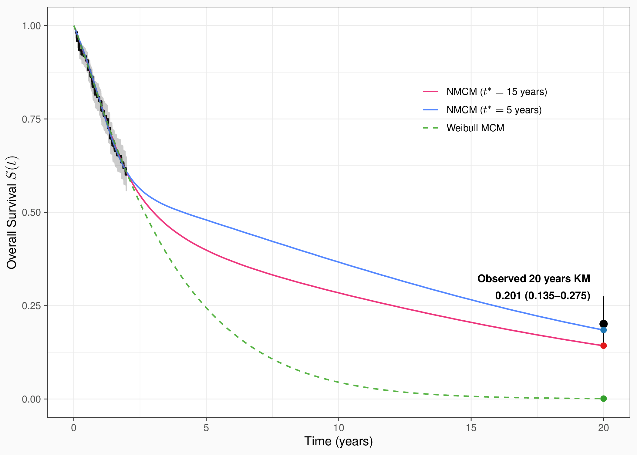
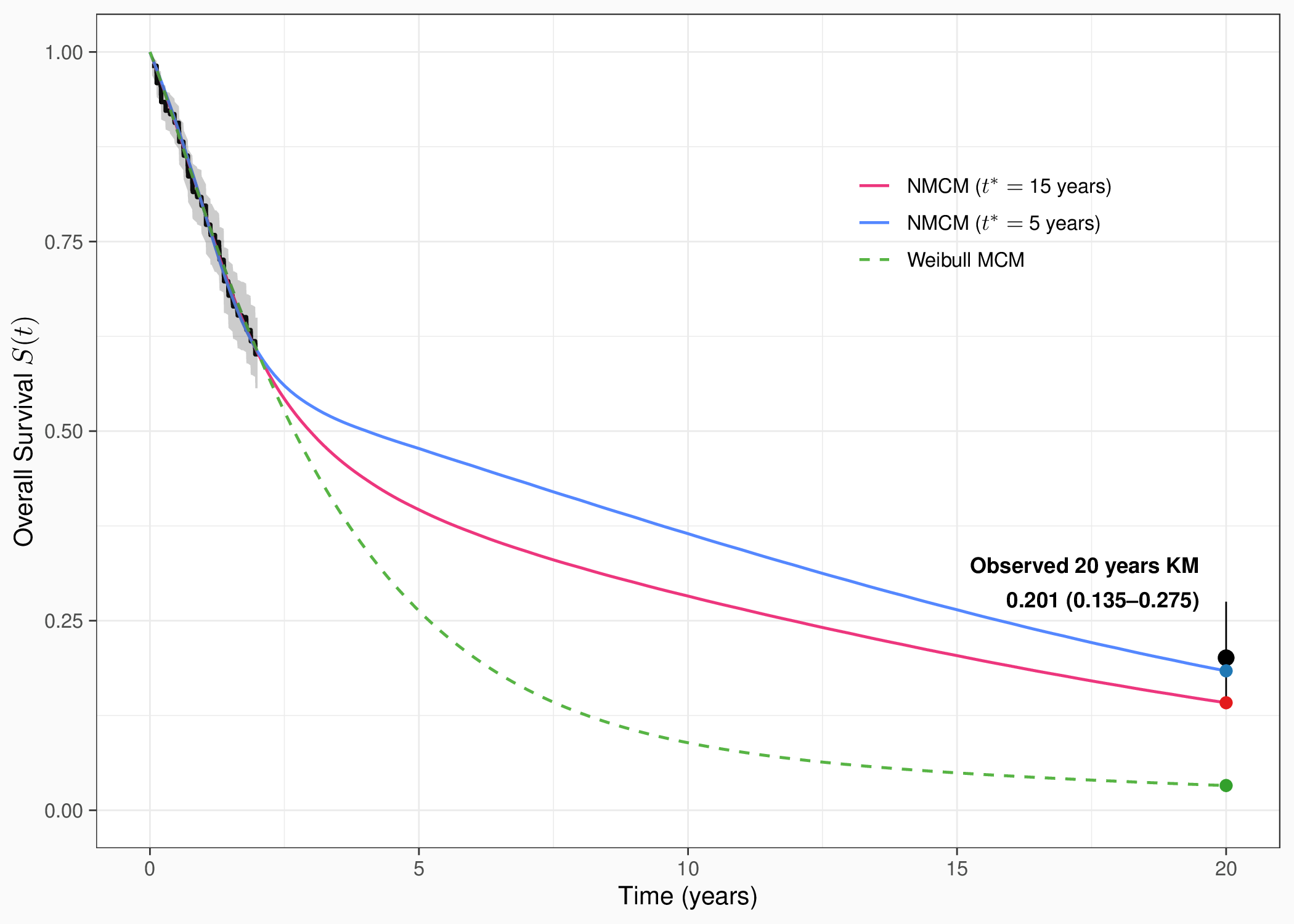
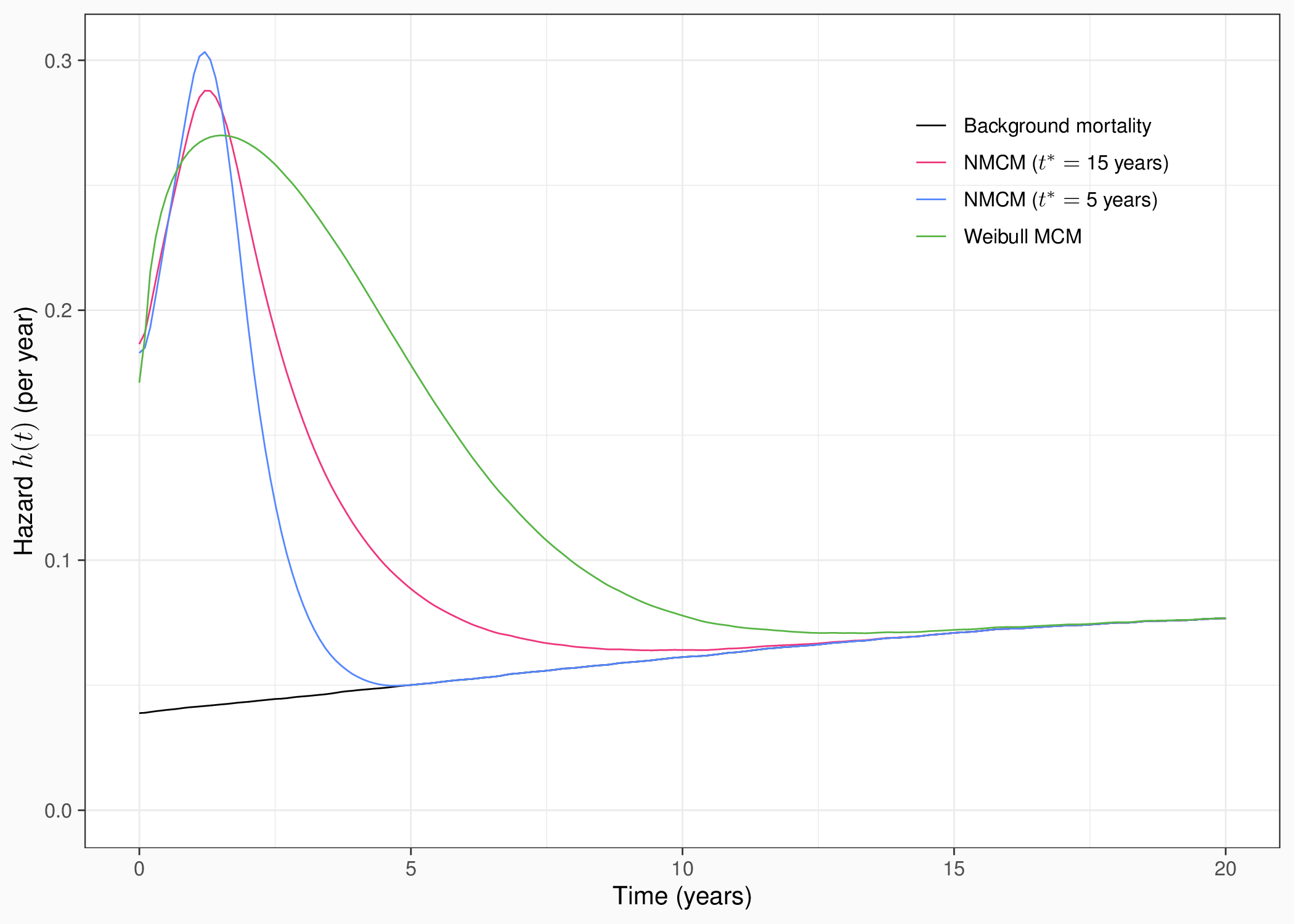
- Latimer & Rutherford’s colon cancer example, medium cure, 24-month cut, subset of full data:
| Model | \(\hat{\pi}\) | \(\hat{S}({\mnum{20}})\) |
|---|---|---|
| Weibull MCM | 0% | 0.2% |
| NMCM, 5 years knot | 62% | 19% |
| NMCM, 15 years knot | 49% | 15% |
| Observed | 20.1% (13.5-27.5) |
- Excess hazard tends to drop before \(t^*\), so earlier knots risk assuming premature cure
- Treat \(t^*\) as a clinically elicited sensitivity parameter, not a parameter to optimize
- In this case, clinical expertise still favours 15 years knot as “best” model…
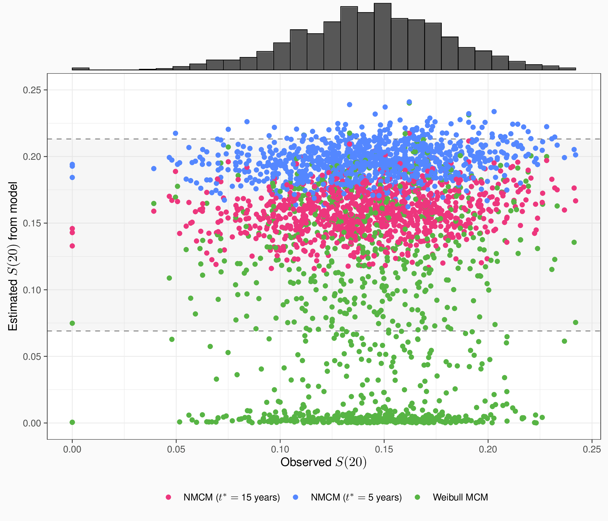
- NB: Controlling for age pushes the Weibull estimate of \(S({\mnum{20}})\) up to 5.7%, but NMCMs essentially unchanged
- NMCM much less sensitive to data variations
- Particularly the 15 years knot model, here…
Bayesian hierarchical MCM
Naïve fit and CFL are two extremes. Let the data decide how much PFS and OS should agree.
Treatment \(k\), endpoints \(j = {\mnum{1}}, {\mnum{2}}\) (PFS, OS)
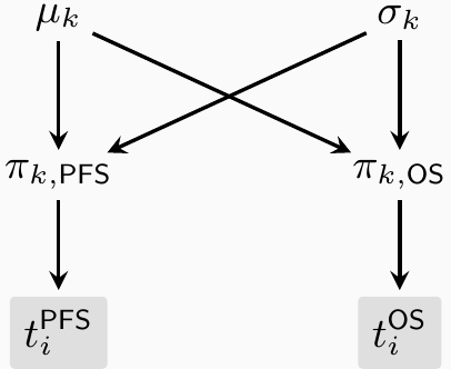
Hyperprior linking cure fractions across endpoints: \[ \begin{aligned} S_{kj}(t) & = S^*(t) \left[\pi_{kj} + ({\mnum{1}}-\pi_{kj})\, S^{j}_{u}(t)\right] \\ \logit(\pi_{kj}) & \sim \dnorm\left(\mu_k, \sigma_k^{\mnum{2}}\right) \end{aligned} \]
- \(S^*(t)\) from life tables, depending on individual covariates
- \(\mu_k, \sigma_k\): shared parameters, linking \(\pi_{k,\txt{PFS}}\) to \(\pi_{k,\txt{OS}}\)
- \(\sigma_k\) estimated from the data \(\;\Rightarrow\;\) modulates borrowing (NB: needs sensible priors!…)
- Three regimes, one model:
- \(\sigma_k \to {\mnum{0}}\): \(\pi_{k,\txt{PFS}} = \pi_{k,\txt{OS}}\) \(\;(\approx\) CFL\()\)
- \(\sigma_k \to \infty\): independent \(\;(\equiv\) naïve MCM\()\)
- Intermediate \(\sigma_k\): soft link
- Full posterior \((\pi_{kj}, \mu_k, \sigma_k, \ldots)\;\Rightarrow\;\) PSA
Software: multimcm
https://github.com/StatisticsHealthEconomics/multimcm
Green N, Kurt M, Moshyk A, Larkin J, Baio G. (2025) A Bayesian Hierarchical Mixture Cure Modelling Framework to Utilize Multiple Survival Datasets for Long-Term Survivorship Estimates: A Case Study From Previously Untreated Metastatic Melanoma. Statistics in Medicine, 44(13-14):e70132. https://doi.org/10.1002/sim.70132
CheckMate 067: melanoma case study
1L metastatic melanoma (nivo+ipi, nivo, ipi); PFS + OS; fit at 12/30/60 month artificial data-cuts.
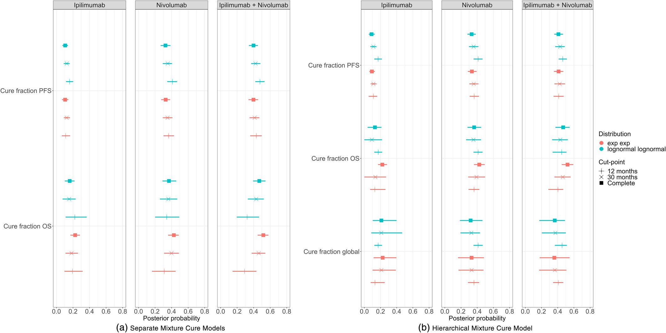
- At 12 months (immature OS): separate MCM cure fractions swing wildly across parametric families; hierarchical stable, close to the 60-month “answer key”
- At 60 months (mature): separate and hierarchical agree