Check out our departmental podcast “Random Talks” on Soundcloud!
Follow our departmental social media accounts + magazine “Sample Space”
Department of Statistical Science | University College London
Disclaimer
This presentation is a summary of the work conducted in Work-Package 4
I can take all the credit (😉), but in reality, this has been driven by the fantastic work of Ioannis Rotous
Key contributions to this work have arrived from all the other EPITOME researchers (e.g. in discussions for the methodological framework to represent the underlying processes, as well as for the formalisation of the statistical modelling)
EPITOME
Evaluating Policy Implementation TO Predict MEntal health: a Bayesian hierarchical framework for quasi-experimental designs in longitudinal settings
WP1: hierarchical statistical framework
Core Bayesian time series model with spatial/temporal dependency, extended to stepped wedge and matched-control designs
Simulation study to assess robustness and sensitivity to model and prior choices
WP2: evaluating impact on mental health need in England
Apply the framework to five UK datasets to estimate effects of Universal Credit and the Hostile Environment Policy
Test for independent and combined effects across socioeconomic and ethnic minority groups
WP3: developing alternative controls
Develop Bayesian synthetic control and negative outcome control methods for cases with no standard control group
Apply these to the WP2 case studies and extend simulations to guide their use
WP4: economic evaluation
Extend existing forecasting models into a Bayesian framework, propagating uncertainty from WP1 to WP3
Use multi-state modelling and potentially Value of Information analysis to assess service demand and decision adequacy
Background
Context
The Legacy Welfare (LW) system is a complex, post-WWII evolved safety net that often required multiple, non-integrated applications for different areas of support
The 2010s policy shift aimed to replace this administrative complexity with Universal Credit (UC) – a single, integrated payment structure
Primary Policy Aims:
Efficiency. Streamline administration to reduce system errors and fraud
Incentive. Create a “work-first” culture by smoothing the transition from benefit dependency to employment
Simplicity. Reduce the burden on claimants to navigate multiple government agencies
Research gap & objectives
No previous research has modelled the dynamic co-evolution of benefit status and well-being
In addition, existing literature generally has not quantified the trade-off between government expenditure and long-term socioeconomic outcomes
Objective: conduct the first formal economic evaluation comparing UC to LW
Use Health Technology Assessment (HTA) tools to map the entire “welfare trajectory”, not just individual symptoms
Health technology assessment (HTA)
Objective
Combine costs and benefits of a given intervention into a rational scheme for allocating resources
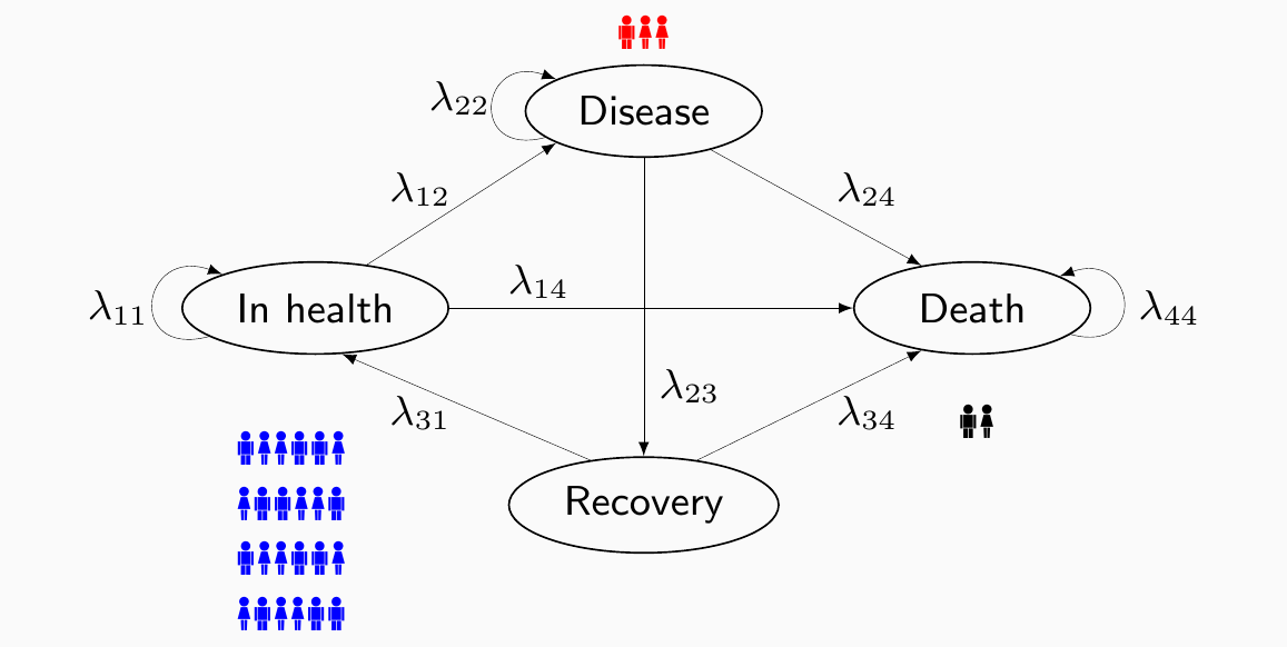
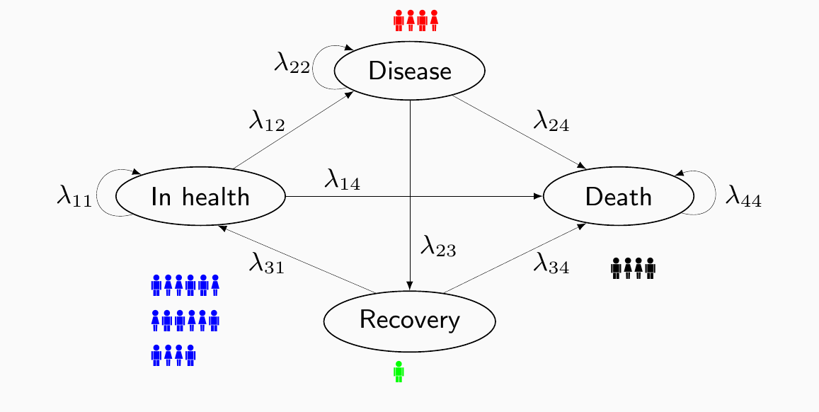
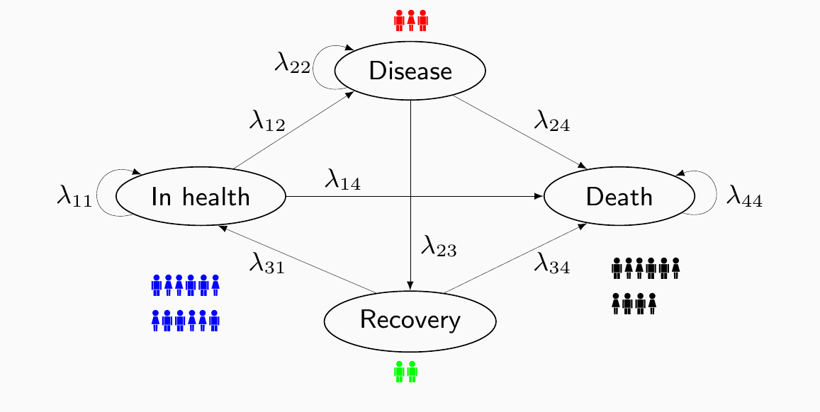
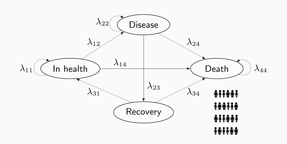
Multi-state/Markov models
Assume a set \(\mathcal{S}\) made of \(S\) “clinically relevant” states
Exhaustive and mutually exclusive
The structure (links among nodes) describes the dynamics of disease history
Links connecting two states encode the assumption that a transition from the one where the link originates to the one reached by it is possible
Absence of a link between two states implies that the transition from one to the other is not allowed by the model
From one period to the next, subjects can move across the states according to the rules specified by the links
Movements occur according to suitable transition probabilities\[\color{#24568c}\bm\pi_j = \bm\pi_{j-1} \bm\Lambda_j\] where
\(\bm\pi_j=(\pi_{1j},\ldots,\pi_{Sj})\) is the vector of probabilities for each state at time \(j\)
\(\bm\Lambda_j = [\Lambda_{j;s',s}]\) is a transition matrix describing the probability of moving from state \(s\) to state \(s'\) at time \(j\)
NB the matrix algebra simply computes for each state \(s\)
\[\color{blue}{\Pr(\style{font-family:inherit;}{\text{Being in state }} s \style{font-family:inherit;}{\text{ at time }} j)= \sum_{s'\in\mathcal{S}}\Pr(\style{font-family:inherit;}{\text{Being in state }} s' \style{font-family:inherit;}{\text{ at time }} j-1)\times \Pr(\style{font-family:inherit;}{\text{Moving from state }}s'\style{font-family:inherit;}{\text{ to state }}s)}\]
Multi-state/Markov models
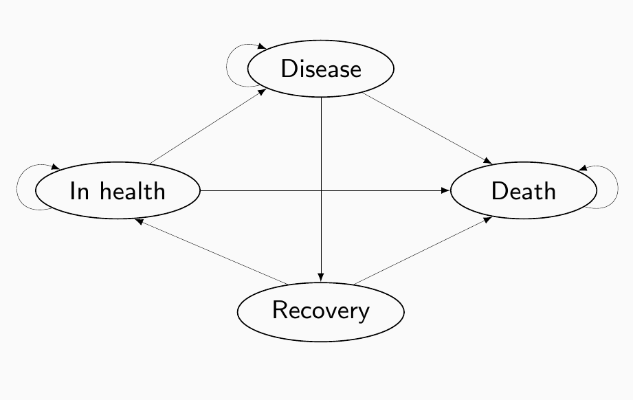
1. Define a structure (e.g. “Natural history” of the disease)
Multi-state/Markov models
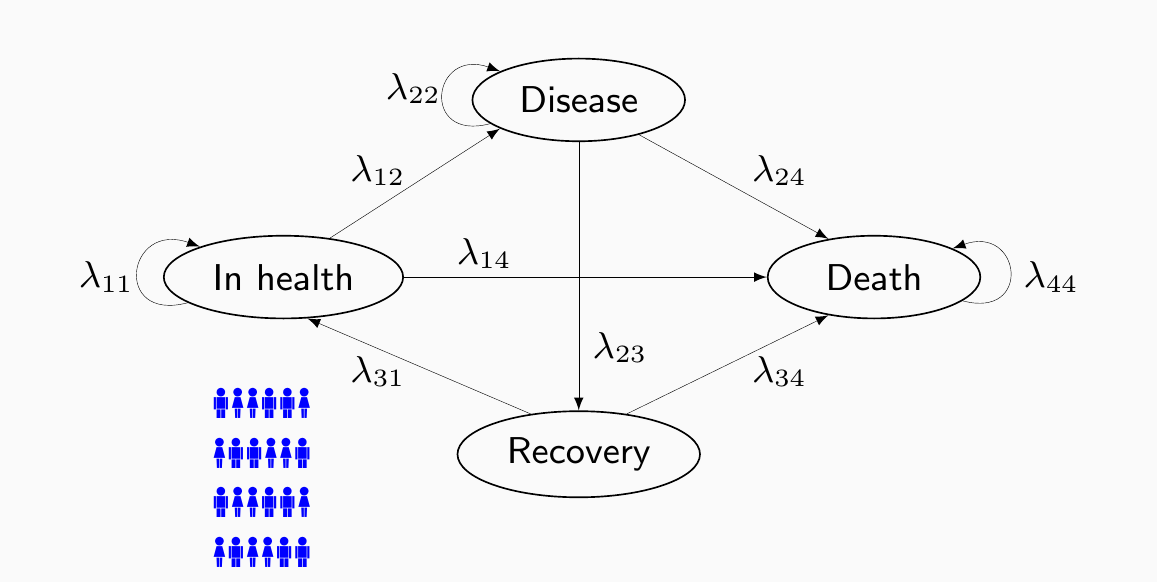
2. Estimate the transition probabilities
For instance:
\(\lambda_{14} =\) general (healthy) population mortality \(\Rightarrow\) Relevant data: Life tables/official records, . . .
Focus on working-age (16-64) individuals in Great Britain
Exclude those with pre-existing lifetime illnesses or disabilities to ensure results reflect policy impacts rather than health crises
Stratified sampling design: 108 geographical strata, with primary sampling units (PSUs) selected on either postcode sectors or groups of postcode sectors and systematic sampling within each PSU
Study cohorts:
Universal Credit (6%): exposed to UC between 2013-2020
Legacy Welfare (40%): exclusive to the old benefit system
No Benefit (54%): never claimed support
NB: UC rollout was administratively mandated, not triggered by personal life shocks, allowing us to evaluate the effects of the policy change
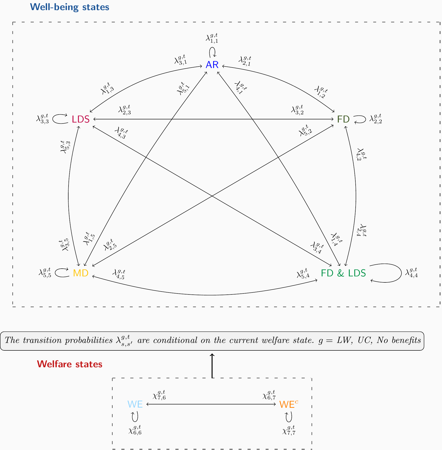
Multi-state modelling for the UC/LW evaluation
Layer 1 – Welfare states: a binary classification of either Welfare Exit (6) or Welfare Entry (active claim; 7)
Layer 2 – Well-being states: five distinct states of human experience:
At Risk; 1 (Baseline): hardship-free
Distress States: Financial Distress (2), Life Dissatisfaction (3), or Combined (4) (Both)
Mental Distress (5): clinical endpoint (GHQ-12)
Well-being pathways are conditional on welfare status
The welfare layer modulates how individuals transition through the well-being states
Assumes welfare status drives well-being outcomes rather than the other way around \(\Rightarrow\) isolates the policy’s direct impact
Simulate 5,000-person cohort year-by-year (2009-2020) to calculate the cumulative time spent in “Distress” vs “Hardship-Free” states
Bayesian Multinomial-logistic ITS: \(w\)elfare status
For individuals \(i = 1, 2, \ldots, n\), residing in a LSOA region \(r_{i}\), belonging to a stratification group \(k_{i}\), assigned to a PSU group \(\psi_{i}\) and observed over time points \(t\)\[
\begin{aligned}
\text{Pr}(Y^{(w),i,t} & = q\mid Y^{(w),i,t-1} = q') = \frac{e^{\eta_{q',q}^{i,t}}}{\sum_{q=6}^{7}e^{\eta_{q',q}^{i,t}}} = \chi_{q',q}^{i,t}, \ \txt{with} \ \ \chi_{q',6}^{i,t} + \chi_{q',7}^{i,t} = 1, \\[10pt]
\logit({\chi}_{q',q}^{i,t}) = {{\eta}_{q',q}^{i,t}} = & {\color{olive}\beta_{0}^{q}} + {\color{red}\beta_{1}^{q}}\txt{Age}_{i,t} +{\color{red}\beta_{2}^{q}} \txt{HEQ}_{i,t}+ {\color{red}\beta_{3}^{q}}\txt{ETH}_{i,t} + {\color{red}\beta_{4}^{q}}\txt{MS}_{i,t} + {\color{red}\beta_{5}^{q}}\txt{Sex}_{i,t} + {\color{red}\beta_{6}^{q}}\txt{GR}_{i,t} + \\
& {\color{orange}f^{q}_{\txt{Exposed}^{i}}(t)} + {\color{orange}f^{q}_{\txt{Intervention}^{i,t}}} + {\color{blue}\gamma_{r_{i}}^{q}} + {\color{blue}\nu_{k_{i}}^{q}} + {\color{blue}\zeta_{\psi_{i}}^{q}} + {\color{purple}\delta_{t}^{q}} + {\color{purple}e_{i}^{q}}
\end{aligned}
\]
Destination-specific baseline log-odds
Confounding factors: age, highest education qualification, ethnicity, martial status, sex and Government Office region
Structured terms
Random effects by stratification group, PSUs and LSOAs to control for neighborhood and regional variations (ensuring results are not just reflecting local geography)
Random effects to account for temporal variability and individual heterogeneity
Cubic B-splines to map complex, non-linear population changes across the 2009-2020 timeline
Bayesian Multinomial-logistic ITS: \(w\)ell \(b\)eing status
Confounding factors: age, highest education qualification, ethnicity, martial status, sex and Government Office region
Structured terms
Random effects by stratification group, PSUs and LSOAs to control for neighborhood and regional variations (ensuring results are not just reflecting local geography)
Random effects to account for temporal variability and individual heterogeneity
Cubic B-splines to map complex, non-linear population changes across the 2009-2020 timeline
Benefits effect: shifts the log-odds of a well-being transition if the individual is currently receiving benefits (= in state \(q=7\))
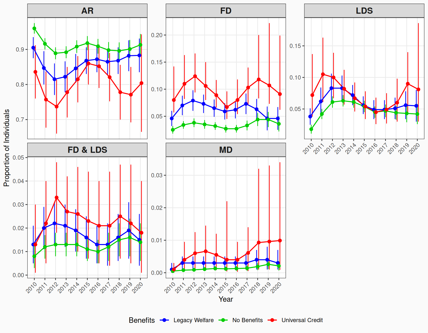
UC claimants spend significantly more time in adverse states than the LW cohort
UC claimants show a substantial increase in life-years spent in Financial Distress
UC increases the probability of transitioning into and staying in Mental Distress and Life Dissatisfaction
The longer an individual remains on UC, the more negative probabilities compound, reducing time spent in the “At-Risk” (hardship-free) baseline
UC creates a “sticky” environment that systematically degrades claimant resilience over time
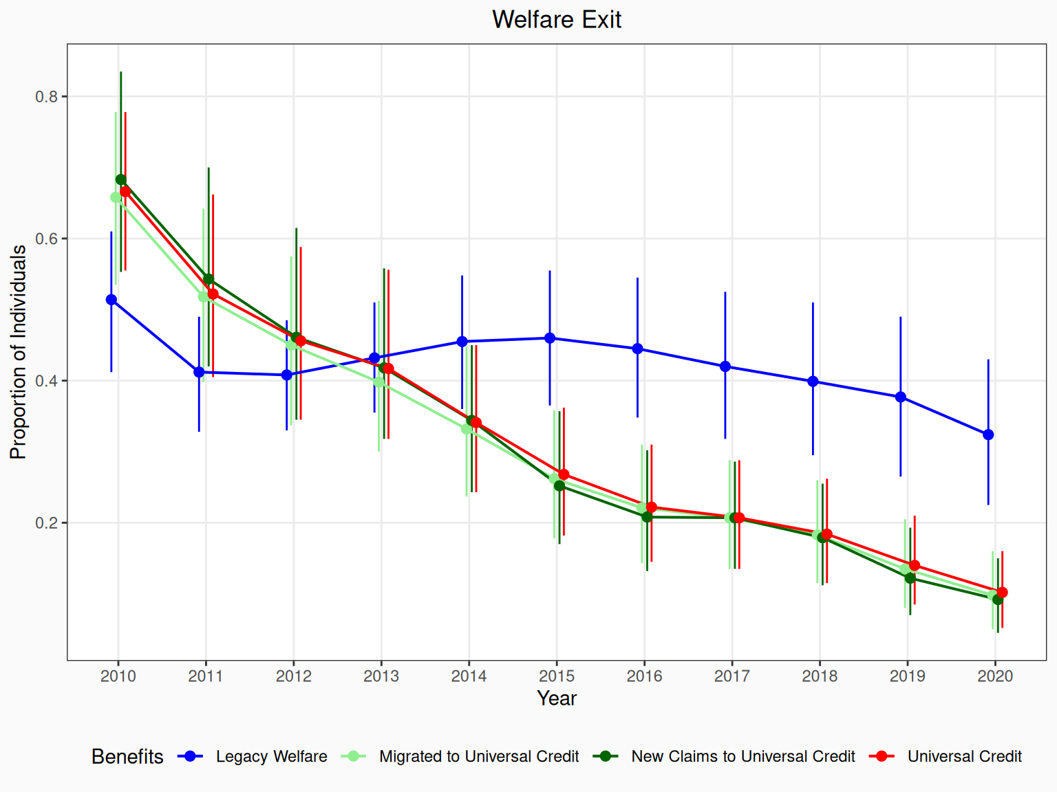
Welfare exit rates over time
Performance measured by fluidity: how effectively a system helps claimants transition off benefits (Welfare Exit) vs keeping them trapped (Welfare Entry)
UC triggered a sharp, continuous drop in welfare exit rates starting in 2013-2014, falling far below the stable exit rates of LW
Low exit rates affect both migrated and new claimants, proving the decline is a systemic feature of UC rather than just a result of personal life shocks
Drop in exit capacity is universal across genders, but is most severe among male new claimants
Instead of acting as an empowering bridge to work, UC introduces structural barriers that prolong welfare reliance
Economic evaluation
Adapts standard Health Technology Assessment (HTA) principles to measure the financial cost per unit of human well-being achieved by each system
Benefits = expected number of life-years an individual spends in the completely hardship-free At Risk (AR) baseline state
Costs = total cost for those in receipt of benefits
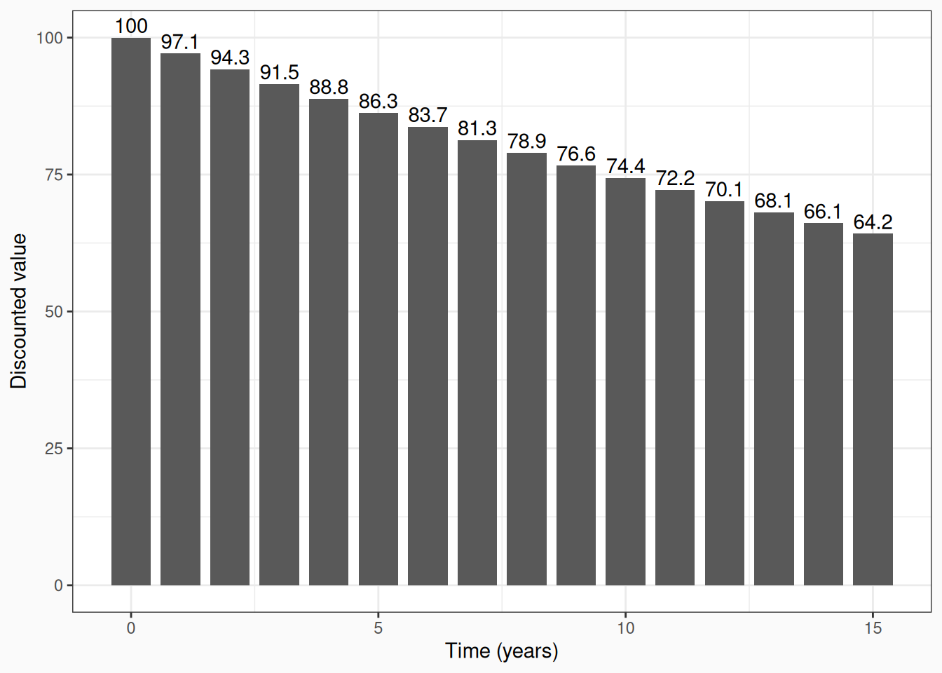
Both discounted at 3.5% yearly, in line with NICE suggestions
Posterior sample summaries of the mean and 95% credible interval of costs in millions of pounds, life-years spent on AR, change in costs, change in benefits, and the ICER between UC and LW
Cost (£1m)
Benefit
Differential Cost \(\Delta_c\)
Differential Benefits \(\Delta_e\)
ICER
UC
120 (104, 131)
3.35 (2.72, 3.92)
-
-
-
LW
72 (56, 86)
3.87 (3.32, 4.50)
47 (35, 59)
-0.51 (-0.94, -0.15)
-92
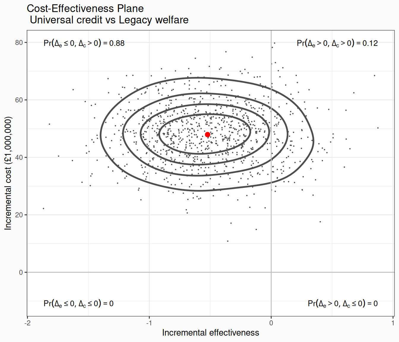
Core findings (2013-2020):
UC claimants spent an average of 0.51 fewer life-years in a hardship-free state compared to LW
The transition to UC cost the government an additional £47 million across the study period
The Incremental Cost-Effectiveness Ratio (ICER) \(=\displaystyle \frac{\txt{E}[\Delta_c]}{\txt{E}[\Delta_e]}\) is strictly negative: UC is “dominated” by the legacy system, meaning it delivers significantly worse human outcomes at a higher taxpayer cost
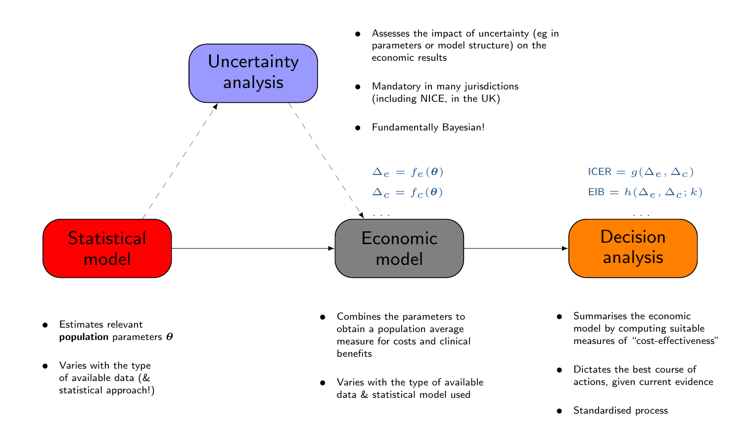
Uncertainty analysis
Study limitations
Uniform cost assumptions
The economic calculations assume a uniform expenditure per individual because precise, individual-level cost data were unavailable
Undifferentiated welfare exits
The data allow the model to track when individuals exit the benefit system, but it cannot differentiate whether they exited due to positive reasons (like improved financial circumstances) or negative reasons (like system disengagement or sanctions)
Masked heterogeneity
The model does not incorporate interaction terms between UC intervention and demographic covariates
Consequently, it may mask how specific groups, such as older claimants who might struggle with the system’s digital design, experience more pronounced adverse effects than the average
Unidirectional causality
The Cohort Markov Model is structurally limited by an assumption of unidirectional causality
It measures how welfare status influences well-being, but it does not capture the reverse effect, such as how a sudden deterioration in well-being might independently prompt someone to exit the welfare system
Policy implications & conclusion
Empirical evidence contradicts foundational claims that UC effectively streamlines the safety net, reduces poverty or eases transitions to financial independence
In fact, UC operates as a “dominated” policy intervention, simultaneously increasing government expenditure while decreasing claimant well-being and hardship-free life-years
Built-in features like the mandatory five-week initial wait time and punitive sanction regimes act as direct structural drivers of chronic financial and mental distress
Core policy recommendations:
Eliminate Structural Bottlenecks: replace or heavily subsidize the initial five-week wait with non-repayable starter grants
Reform punitive sanctions to focus on supportive, health-conscious employment integration
Future welfare design must move past purely administrative and fiscal-tightening metrics
Social safety nets should instead be evaluated using holistic, health-economic frameworks prioritizing long-term claimant resilience
Bayesian inference needs the posterior \(p(\theta \mid y)\), but exact computation is often intractable and MCMC can be too slow for large or complex models
Variational inference (VI) turns inference into optimisation
Since \(\txt{KL}>0\) and \(p(y)\) is constant (wrt to \(\phi\)), maximising \(\txt{ELBO}(\phi)\) is equivalent to minimising \(\txt{KL}\left(q_\phi \mid\mid p(\theta \mid y)\right)\)
Stan transforms constrained parameters to an unconstrained space, then use a Normal distribution for \(q_\phi\)
Optimisation uses automatic differentiation, so no model-specific derivation is needed
Much faster than MCMC, but approximated inference
In complex cases, might understate uncertainty, with no general convergence guarantee